RQM description of the charge form factor
of the pion and its asymptotic behavior

Abstract

The pion charge and scalar form factors, $F_{1}(Q^{2})$ and $F_{0}(Q^{2})$, are first calculated in different forms of relativistic quantum mechanics. This is done using the solution of a mass operator that contains both confinement and one-gluon-exchange interactions. Results of calculations, based on a one-body current, are compared to experiment for the first one. As it could be expected, those point-form, and instant and front-form ones in a parallel momentum configuration fail to reproduce experiment. The other results corresponding to a perpendicular momentum configuration (instant form in the Breit frame and front form with $q^{+}=0$) do much better. The comparison of charge and scalar form factors shows that the spin-1/2 nature of the constituents plays an important role. Taking into account that only the last set of results represents a reasonable basis for improving the description of the charge form factor, this one is then discussed with regard to the asymptotic QCD-power-law behavior $Q^{-2}$. The contribution of two-body currents in achieving the right power law is considered while the scalar form factor, $F_{0}(Q^{2})$, is shown to have the right power-law behavior in any case. The low-$Q^{2}$ behavior of the charge form factor and the pion-decay constant are also discussed.

PACS numbers: 12.39.Ki, 13.40.Fn, 14.40.Aq
Keywords: Relativistic quark model; Form factors; Pion

1 Introduction

The pion has a double interest. As a physical system, it allows one to learn about its hadronic structure and how QCD is realized. As a test case, it can be used to check methods to describe properties of strongly interacting systems. Its charge form factor, which has been measured up to $Q^{2}\simeq 10$ (GeV/c)² [1, 2, 3, 4, 5, 6], has thus been the object of a lot of attention. Noticing that the distinction is not always relevant as soon as some approximations are made, it has been considered in both field-theory [7, 8, 9, 10, 11, 12, 13] and relativistic-quantum-mechanics (RQM) approaches [14, 15, 16, 17, 18, 19, 20, 21, 22, 23, 24, 25]. Most often, results have been obtained and analyzed within the standard light-front formalism ($q^{+}=0$).

Recently, more extensive studies looking at the role of various momentum configurations within field-theory approaches, with the transfer momentum parallel or perpendicular either to the average momentum of the system or to the front-orientation, have been made [11, 12, 13]. A large sensitivity to various one and two-body contributions was observed though the total result is well determined. Not much attention was however given to these results, perhaps because the momentum configuration $q^{+}=0$ generally imposes itself as the most appropriate.

The situation in relativistic quantum mechanics is somewhat different. On the one hand, in absence of a close relationship to field theory, there are currently discussions as to which wave function or/and which current will be the best to reproduce experimental data [15, 20, 23, 24]. The only study that tried to incorporate a more founded wave function [16, 17] failed to account for the measurements of the pion charge form factor and, in this order, was forced to invoke quark form factors. These ones could account for some missing physics which is expected to play some role like that one underlying the vector-meson-dominance phenomenology. On the other hand, it appeared that the estimate of this observable [22, 24] could be very sensitive to the form employed in implementing relativity [26], quite similarly to what was observed for spinless constituents [27]. Moreover, an extension of this last work [28] showed a strong sensitivity of instant and front-form results to the momentum configuration, like in field-theory based approaches [11, 12, 13]. It would not be surprising whether a similar effect shows up in the pion case too. Altogether, there are therefore many reasons for motivating further studies of the pion charge form factor within relativistic quantum mechanics. One could add that specific predictions from QCD relative to the asymptotic pion charge form factor [29, 30, 31] or to the Goldstone nature of the pion have been hardly discussed within the RQM framework.

When looking at the pion form factor within relativistic quantum mechanics approaches, further work could be motivated by the numerous differences that are expected with the scalar-particle case considered in previous works [32, 27, 28]. Apart from the fact that the relevance for a physical system of conclusions achieved for an academic one has been questioned, the spin-1/2 nature of the constituents represents an important if not a major difference as will be seen. This can affect the solution of a mass operator, the current (Lorentz vector or Lorentz scalar) and, ultimately, the charge and Lorentz-scalar form factors as well as their asymptotic behavior. Confinement represents another difference characterizing hadronic physics. How these differences show up when comparing form factors calculated in different forms (and different momentum configurations) together with a single-particle current is to be determined. This is our first goal.

Anticipating that a reasonable starting point for further improvement is only given by the standard instant- and front-form approaches (Breit-frame and $q^{+}=0$ respectively), a second goal is to determine the role of two-body currents in getting the right $Q^{-2}$ QCD asymptotic behavior for the pion charge form factor within these approaches [30, 31]. Addressing this question in a RQM framework may look premature. Apart from the fact it should be ultimately considered, we notice that previous work with scalar particles succeeded relatively easily to reproduce the expected power-law behavior of form factors in the standard instant- and front-form approaches [27, 28]. This gives us some confidence in considering the problem here. It involves the interaction at short distances, due to one-gluon exchange and, of course, the spin of the constituents. With this respect and though there is no known scalar probe of practical relevance, the consideration of the scalar form factor, beside the charge one, is especially useful in revealing features specific to their asymptotic behavior. The contribution of two-body currents was considered in the past with the aim to restore the appropriate asymptotic behavior but this was for a calculation involving the “point form” approach and scalar constituents [33]. Moreover, the origin of a wrong asymptotic behavior in this last approach differs from the one considered here for the pion in the standard instant- and front-form approaches.

While considering the two goals mentioned above, we found that the main trends evidenced by the results were rather insensitive to various ingredients entering the mass operator. Quantitatively, some sensitivity was observed however. We will therefore present here the main lines, leaving for future work a more complete discussion of the quantitative aspects. With this last respect, we will only mention the points that could be questionable. Preliminary results were presented in ref. [34] while the role of different forms was recently discussed by He et al. [24], using phenomenological wave functions.

The plan of the paper is as follows. In the second section, we consider the description of the pion in different forms. We, in particular, discuss the mass operator which contains both a confining part and a Coulomb one. The expression of the charge and scalar form factors in different forms is given in the third section. One-body and some two-body currents are considered. The expression of the pion-decay constant, $f_{\pi}$, is also discussed as well as quantities that involve this constant, namely the charge form factor in the asymptotic domain and the charge radius (with some approximation). The fourth section is devoted to the presentation of the results with the one-body current and to their discussion, for the low- as well as the high-$Q^{2}$ range. The analysis of the asymptotic form factor is considered in the fifth section. The conclusion and further discussion is given in the sixth section. Three appendices contain details about accounting for the spin-1/2 nature of the constituents in the mass operator, the behavior of the solution at short distances for a strong Coulomb-type interaction, and about two-body currents contributing to the charge form factor.

2 Pion description in different forms

Prior to any calculation of form factors in relativistic quantum mechanics, two ingredients have to be specified. On the one hand, a mass operator, whose solutions could be used in different forms, is needed. On the other hand, the relation of the momenta of the constituent particles to the total momentum, which depends on the form, is required. They are successively discussed in this section.

2.1 Mass operator

We here follow a previous work based on a quadratic mass operator together with a single-meson-exchange type interaction [27]. This approach, specialized to scalar particles, was able to provide a good account of form factors corresponding to an “exact” theoretical model in both the instant- and front-form approaches. In the case of an infinite-mass exchange interaction, the “exact” form factor could be reproduced, ensuring the correctness of a minimal number of ingredients for both the mass operator and the currents. In the pion case, two further ingredients have to be considered: the spin-1/2 nature of the constituents and confinement. A mass operator that accounts for these features is the following:

$$M^{2}_{\pi}\;\phi_{0}(k) = \Big{(}(2\,e_{k}+\sigma_{st}\;r-V_{D})^{2}+\Delta\Big{)}\;\phi_{0}(k)$$ (1)

$$-\int\;\frac{d\vec{k}^{\prime}}{(2\,\pi)^{3}}\;\frac{4\;g_{eff}^{2}\;\frac{4}{3}\;e_{k}\;e_{k^{\prime}}\Big{(}2-\frac{m^{2}_{q}\,(e^{2}_{k}+e^{2}_{k^{\prime}})}{2\,e^{2}_{k}\;e^{2}_{k^{\prime}}}\Big{)}}{\sqrt{e_{k}}\;\;(\vec{k}-\vec{k}^{\prime})^{2}\;\;\sqrt{e_{k^{\prime}}}}\;\phi_{0}(k^{\prime}),$$

where $e_{k}=\sqrt{m_{q}^{2}+k^{2}}$. The spinor part of the pion wave function factors out and has therefore been omitted in writing the above equation (see appendix A for some detail). The only but important effect due to the spin-1/2 nature of the constituents, in comparison with the scalar-particle case, is the replacement in the last term of a factor $m^{2}$ by $e_{k}\;e_{k^{\prime}}\;\Big{(}2-m^{2}_{q}\,(e^{2}_{k}+e^{2}_{k^{\prime}})/(2\,e^{2}_{k}\;e^{2}_{k^{\prime}})\Big{)}$. The equation being written in momentum space, the distance $r$ should be considered as an operator. In order to simplify the writing of some expressions later on, we also introduce a wave function defined differently, $\tilde{\phi}(k)=\sqrt{e_{k}}\;\phi_{0}(k)$.

The confinement term together with the kinetic-energy one appears in a quadratic form, in accordance with the quadratic character of the mass operator. This model [35] can roughly reproduce the Regge trajectories and the first radial excitations of mesons with a string tension $\sigma_{st}=0.2\;$GeV² and $V_{D}=0.486$ GeV. The other part of the interaction is inspired from the single-gluon exchange one. It incorporates the standard Coulomb part but it also involves non-relativistic corrections that are usually omitted (see appendix A). It contains the QCD coupling, here replaced by an effective one, $g_{eff}^{2}/4$, and a factor $16/3$ representing the value taken by the color matrices for a meson. In accordance with the way we derive this part of the interaction, there is no specific contribution due to the standard spin-spin term. This one is actually cancelled in the present case by a term with the same spatial structure, generally omitted. The above effective one-gluon exchange interaction could a priori have a more complicated expression. In absence of a detailed study, we assumed the simplest choice compatible with reproducing the one-gluon exchange in the perturbative regime, the only parameter being the effective coupling, $g_{eff}^{2}/4$. Once the above ingredients are fixed, the pion mass can be reproduced by choosing appropriately the quantity, $\Delta$. The equation can be solved in various ways. Working here in momentum space, we consider the operators $\sigma_{st}\;r$ and $(\sigma_{st}\;r)^{2}$ as the limit for $G$ going to infinity of the quantities, $G\;(1-{\rm exp}(-\sigma_{st}\;r/G))$ and $G^{2}\;(1-{\rm exp}(-(\sigma_{st}\;r/G)^{2}))$, and Fourier transform them. The solution is expected to have the high-momentum behavior, $\phi_{0}(k)\propto k^{-7/2}$, up to log corrections. For a strong enough coupling, these corrections can lead to a change of the power-law behavior. One thus expect $\phi_{0}(k)\propto k^{-3}$ for $(8/3)\;g_{eff}^{2}/(4\,\pi)=0.5$ (see appendix B). A critical regime could be reached when this quantity takes the value $2/\pi$ [36], which is in the range of expectations when the current QCD coupling, $g_{eff}^{2}/(4\,\pi)=\alpha_{s}$, is used. The power-law behavior of $\phi_{0}(k)$ is quite important as it determines that one for form factors [37], unless some specific suppression occurs in relation with a particular probe.

For practical purposes, we use $m_{q}=0.2\;$GeV, $M_{\pi}=0.14\;$GeV, $\sigma_{st}=1\;$GeV/fm$=0.2\;$GeV² and $V_{D}=0.5$ GeV. For the strong QCD coupling, we distinguish two regimes, a low- and a high-energy one. In the first case, the effective coupling is taken as $(8/3)\;g_{eff}^{2}/(4\,\pi)=0.5$, which corresponds to the case mentioned above where the wave function should scale like $k^{-3}$ at large $k$. This coupling value is somewhat a compromise between larger and smaller values expected respectively in the low- and high-energy regime (see also below for other effects). In the second case, anticipating on the fact that the coupling should go to 0, it was assumed that the solution behaves like $k^{-7/2}$ for $k\geq$5.6 GeV. As a result of these choices, the behavior of our solution slowly changes from the behavior $k^{-3}$ obtained around 1 GeV to the one ascribed beyond 5.6 GeV. One then obtains the value of the last parameter, $\Delta=-0.487$ GeV².

Being interested here in gross features, we only considered the most important parts of the interaction: the confinement and the one-gluon exchange, which are essential to reproduce respectively the dominant aspects of the hadron spectroscopy and the asymptotic behavior of form factors. We did not therefore try to improve upon the above model. On the one hand, the derivation of the effective interaction to be used in relativistic quantum mechanics is largely open. This has been done to some extent in the scalar-particle case where the effect of retardation was found to lead to an effective coupling 2-3 times smaller than the free one [38]. The estimate of this effect and other ones is likely to be more complicated for the one-gluon exchange interaction [39], of interest here. On the other hand, the running character of the strong QCD coupling, $\alpha_{s}$, should be accounted for. Due to the relatively enhanced weight of high momenta in the solutions of eq. (1), one can anticipate that values of this coupling smaller than those currently referred to for the low-energy domain should be used. An important point is that, in both cases, the most singular part of the interaction, which determines the asymptotic behavior of form factors [40] and is given in eq. (1) by the Coulomb term, be preserved (up to log terms). Of course, the interaction can be improved on a phenomenological basis, by requiring for instance a closer fit of the parameters to the pion radial excitations at 1300 MeV and 1800 MeV or to the pion-decay constant, $f_{\pi}$.

2.2 Constituent and total momenta in different forms: relation

In order to determine the expression of form factors, beside a solution of a mass operator discussed above, the relation of the constituent momenta, $\vec{p}_{1},\;\vec{p}_{2}$, to the total momentum, $\vec{P}$, and the internal variable, $\vec{k}$, is needed. Two ingredients enter their determination. The first one involves the relation of the sum of the constituent 3-momenta and the total momentum:

$$\vec{p}_{1}+\vec{p}_{2}-\vec{P}=\frac{\vec{\xi}}{\xi^{0}}\;(e_{1}+e_{2}-E_{P}),$$ (2)

where $\xi^{\mu}$ characterizes the approach under consideration and, especially, the symmetry properties of the hypersurface which physics is described on. Most often, $\xi^{\mu}$ represents the orientation of a hyperplane and the above equation can then be obtained, up to a phase, by integrating plane waves, ${\rm exp}(i\,(p_{1}+p_{2}-P)\cdot x)$, over the hypersurface $\xi\cdot x=0$. The second ingredient involves a Lorentz-type transformation of the constituent momenta which generalizes that one introduced by Bakamjian and Thomas [41]:

$$\vec{p}_{1,2}=\pm\vec{k}\pm\vec{w}\;\frac{\vec{w}\cdot\vec{k}}{w^{0}+1}+\vec{w}\;e_{k}\;,\;\;\;\;e_{1,2}=w^{0}\;e_{k}\pm\vec{w}\cdot\vec{k}\;,$$ (3)

where $w^{0}=\sqrt{1+\vec{w}\,^{2}}\;(w^{2}=(w^{0})^{2}-\vec{w}\,^{2}=1)$. Combining the two equations allows one to write:

$$w^{\mu}=\frac{P^{\mu}}{2\,e_{k}}+\frac{\xi^{\mu}}{2\,e_{k}}\;\frac{4\,e_{k}^{2}-M^{2}}{\sqrt{(\xi\cdot P)^{2}+(4\,e_{k}^{2}-M^{2})\;\xi^{2}}+\xi\cdot P}\,,$$ (4)

where $w^{\mu}$ depends on the approach through that one of $\xi^{\mu}$. It is noticed that, $\xi^{\mu}$ representing an orientation, its scale is irrelevant, what can be checked on eq. (2) or on the last expression for $w^{\mu}$. The expressions taken by $\xi^{\mu}$ and $w^{\mu}$ are given in the following for different forms.

$\bullet$ Instant-form approach

$$\xi^{\mu}\propto\lambda_{0}^{\mu}\;,\hskip 28.45274pt{\rm with}\;\;(\lambda_{0}^{0},\;\vec{\lambda}_{0})=(1,\;0)\;(\lambda^{2}=1).$$ (5)

$$\vec{w}=\frac{\vec{P}}{2\,e_{k}},\hskip 28.45274ptw^{0}=\frac{\sqrt{4\,e_{k}^{2}+P^{2}}}{2\,e_{k}}\;.$$ (6)

$\bullet$ Front-form approach

$$\xi^{\mu}\propto\omega^{\mu}\;,\ \hskip 28.45274pt{\rm with}\;\;(\omega^{0},\;\vec{\omega})\propto(1,\;\hat{n}),\;(\omega^{2}=0)\,,$$ (7)

$$\vec{w}=\frac{\vec{P}}{2\,e_{k}}+\frac{\hat{n}}{4\,e_{k}}\;\frac{4\,e_{k}^{2}-M^{2}}{E_{P}-\vec{P}\cdot\hat{n}}\;,\hskip 28.45274ptw^{0}=\frac{E_{P}}{2\,e_{k}}+\frac{4\,e_{k}^{2}-M^{2}}{4\,e_{k}\;(E_{P}-\vec{P}\cdot\hat{n})}\;.$$ (8)

where $\hat{n}$ has a fixed orientation.

$\bullet$ Dirac inspired point-form approach [42]

$$\xi^{\mu}\propto u^{\mu}\;,\ \hskip 28.45274pt{\rm with}\;\;(u^{0},\;\vec{u})\propto(1,\;\hat{u}),\;(u^{2}=0)\,,$$ (9)

$$\vec{w}=\frac{\vec{P}}{2\,e_{k}}+\frac{\hat{u}}{4\,e_{k}}\;\frac{4\,e_{k}^{2}-M^{2}}{E_{P}-\vec{P}\cdot\hat{u}}\;,\hskip 28.45274ptw^{0}=\frac{E_{P}}{2\,e_{k}}+\frac{4\,e_{k}^{2}-M^{2}}{4\,e_{k}\;(E_{P}-\vec{P}\cdot\hat{u})}\;.$$ (10)

where $\hat{u}$, contrary to the front-form case, has no fixed orientation.

In the absence of interaction ($2\,e_{k}=M$), the three expressions obtained in different forms for $\vec{w}$ and $w^{0}$ become identical to the standard kinematical boost for free particles. In this limit, one recovers the expressions relevant to an earlier “point-form” approach [43, 44, 45]:

$$\xi^{\mu}\propto\lambda^{\mu}\;,\hskip 28.45274pt{\rm with}\;\;\lambda^{\mu}=P^{\mu}/\sqrt{P^{2}}.$$ (11)

$$\vec{w}=\frac{\vec{P}}{M}\;,\hskip 28.45274ptw^{0}=\frac{E_{P}}{M}.$$ (12)

This “point-form” resembles the Dirac point form in that the dynamical or kinematical character of the Poincaré generators is the same. However, as mentioned elusively by Bakamjian [43] and explicitly by Sokolov [44], this “point-form” implies describing the physics on hyperplanes perpendicular to the velocity of the system and differs from the Dirac one, which involves a hyperboloid surface. The kinematical character of boosts and rotations in the above “point-form” stems from the invariance under Lorentz transformations of the hyperplane defined by the condition that $v\cdot x$ is a constant, where $v$ is the 4-velocity of the system ($v^{\mu}\propto P^{\mu}$). To some extent, the property is trivial as the frame used to describe the system changes at the same time as this one is boosted. A related feature is the fact that it requires a constraint on the interaction much weaker than in the other approaches. When deriving a mass operator, any Lorentz invariant interaction is sufficient while, in the other cases, the consideration of the interaction at all orders is required [42]. A similar statement holds for other quantities such as the charge form factor at $Q^{2}=0$ or the pion-decay constant (see below). The above “point-form” approach thus possesses properties that make it definitively different from the other ones. In some sense, it contains the effect of the boost transformation common to all approaches but without the constraints attached to the fact that the hypersurface which the system is described on is uniquely defined and independent of its velocity. As is well known, this requires interaction effects, represented here by the $\xi^{\mu}$ dependent term at the r.h.s. of eq. (4).

3 Current and form factors

Figure 1: Graphical representation of a virtual photon absorption on a pion together with kinematical definitions.

We consider in this section the pion form factors. There are two of them, corresponding to the coupling to a photon ($F_{1}(Q^{2})$: charge form factor) and to a possible scalar probe ($F_{0}(Q^{2})$: scalar form factor). Their definition we refer to here may be found in ref. [27]. Considering both of them can give a better insight on the implementation of relativity, especially with respect to the non-zero spin of the constituents. The studies are performed on the basis of a single-particle current. Two-body currents will be considered but only for those approaches that already provide a relatively good account of experiment. We therefore discard large contributions from two-body currents that could be required to preserve properties related to the Poincaré space-time translation invariance [28, 46]. In short, these last currents account in a RQM framework for the equality of the momentum that is separately transferred to the constituents and to the whole system, which is fulfilled in field-theory approaches in a straightforward way.

3.1 One-particle current

The form of the single-particle current to be used with the above mass operator has been discussed at length in ref. [27] for spinless constituents. Interestingly, it has been found, since then, that form factors in different forms, due to minimal consistency requirements, could be written in a unique way [28]. They should be completed to account for the spin-1/2 nature of quarks. Referring to fig. 1 for the kinematical notations, they now read:

$$F^{(1)}_{1}(Q^{2})\;\Big{[}F^{(1)}_{0}(Q^{2})\Big{]}=\int\frac{d\vec{p}}{(2\pi)^{3}}\;\;\frac{\xi_{f}\!\cdot\!(p_{f}+p)\;\;\xi_{i}\!\cdot\!(p_{i}+p)}{e_{p}\;(2\,\xi_{f}\!\cdot\!p_{f})\;(2\,\xi_{i}\!\cdot\!p_{i})}\;\;\phi_{0}\Big{(}(\frac{p_{f}-p}{2})^{2}\Big{)}\;\phi_{0}\Big{(}(\frac{p_{i}-p}{2})^{2}\Big{)}$$

$$\times\;\;\Big{(}(p_{f}+p)^{2}\,(p_{i}+p)^{2}\Big{)}^{-1/4}\;\;\;\frac{I\!\cdot\!(\xi_{f}+\xi_{i})}{(p_{f}+p_{i}+2\,p)\!\cdot\!(\xi_{f}+\xi_{i})}\;\;\Big{[}\frac{S}{4\,m_{q}}\;\;cf_{0}\Big{]}.$$ (13)

In this equation, $I^{\mu}$ and $S$ result from the following trace over $\gamma$ matrices:

$$I^{\mu} = 4\;{\rm Tr}\Big{[}\gamma_{5}\;\frac{(m_{q}+\gamma\cdot p_{i})}{2}\;\gamma^{\mu}\;\frac{(m_{q}+\gamma\cdot p_{f})}{2}\;\gamma_{5}\;\frac{(m_{q}-\gamma\cdot p)}{2}\Big{]},$$

$$= 2\;\Big{[}p_{i}^{\mu}\;(p_{f}\cdot p)+p_{f}^{\mu}\;(p_{i}\cdot p)-p^{\mu}\;(p_{i}\cdot p_{f})+m_{q}^{2}\;(p_{i}^{\mu}+p_{f}^{\mu}+p^{\mu})\Big{]},$$

$$S = 4\;{\rm Tr}\Big{[}\gamma_{5}\;\frac{(m_{q}+\gamma\cdot p_{i})}{2}\;\frac{(m_{q}+\gamma\cdot p_{f})}{2}\;\gamma_{5}\;\frac{(m_{q}-\gamma\cdot p)}{2}\Big{]}\,,$$ (14)

$$= 2\;m_{q}\;\Big{[}p_{f}\cdot p+p_{i}\cdot p+p_{i}\cdot p_{f}+m_{q}^{2}\Big{]}\,.$$

In the case of a point-form approach inspired from the Dirac one, it turns out that expressions for form factors can be obtained from the above ones in the front form by integrating them over the orientation of the front together with an appropriate weight. They can be obtained from a straightforward generalization of those for the scalar-particle case [28].

It can be checked that the expression of the charge form factor at $Q^{2}=0$ considerably simplifies. Making an appropriate change of variable, it reduces in all cases to a unique expression:

$$F^{(1)}_{1}(Q^{2}=0)=\int\frac{d\vec{k}}{(2\pi)^{3}}\;\phi^{2}_{0}(k)=\frac{1}{(2\pi)^{3}}\int\frac{d\vec{k}}{e_{k}}\;\tilde{\phi}^{2}(k)=1.$$ (15)

We stress that the result is independent of both the momentum of the system, $\vec{P}$, and the orientation of the hyperplane given by $\xi^{\mu}$, a property which is not trivial in most cases. With this respect, the presence of the factor, $(p_{f}+p_{i}+2\,p)\!\cdot\!\xi$, at the denominator in eq. (13) is essential. This one accounts in a hidden way for some two-body currents [27]. It is also noticed that the above expression of the charge form factor at $Q^{2}=0$ is fully consistent with the expression of the normalization of the solution, $\phi_{0}(k)$, of the mass operator, eq. (1), which involves the same integrand.

In the case of the scalar form factor, and for the instant form, it is generally found that its value at $Q^{2}=0$ depends on the momentum of the system. In other words, it does not verify a minimal Lorentz invariance property. This one can be fulfilled by introducing a correction factor in the expression of the scalar form factor, $F_{0}(Q^{2})$. Denoted $cf_{0}$, this quantity amounts to account for two-body currents. Its expression, whose form is suggested by the consideration of a simple interaction model, has been considered independently [28]. Symmetrizing its effect between initial and final states, it is taken as:

$$cf_{0}=1+\frac{1}{2}\;(g(k_{i})+g(k_{f}))\;e_{p}\;\frac{(e_{f}+e_{p})(e_{i}+e_{p})-E_{f}\;E_{i}}{(e_{f}+e_{p})(e_{i}+e_{p})(e_{f}+e_{i})},$$ (16)

where the function $g(k)$ can be obtained from the following quadrature:

$$\frac{g(k)}{8}\;e_{k}\;(4\,e_{k}^{2}-M^{2})\;\phi^{2}_{0}(k)=\int^{\infty}_{k}dk^{\prime}\;k^{\prime}\;e_{k^{\prime}}\;\phi^{2}_{0}(k^{\prime})\,.$$ (17)

In the case of a scalar-particle model together with a zero-range interaction, $g(k)$ is equal to 1 and the above factor $cf_{0}$ then allows one to reproduce the “exact” scalar form factor, $F_{0}(Q^{2})$.

A few remarks are in order here. A first one concerns the Lorentz-invariance properties of form factors in different forms. While the point-form approaches evidence this property, the instant- and front-forms ones do not. These last approaches can thus be considered for different momentum configurations which include the standard ones (Breit frame and $q^{+}=0$ respectively) but also non-standard momentum configurations like a parallel one where the transfer momentum is oriented along the average momentum of the system ($(\vec{P}_{i}-\vec{P}_{f})\parallel(\vec{P}_{i}+\vec{P}_{f})\parallel\vec{n};\;E_{i}\neq E_{f}$). Their comparison could be instructive but this supposes that no other symmetry is significantly broken at the same time, which has to be checked. A second remark concerns the expressions of form factors in the front-form case. The current ones, generally given in terms of the Bjorken variable, $x$, and the transverse momentum, are recovered from eq. (13) by making a change of variable. The last remark concerns the calculation of form factors in the earlier “point-form”. As the initial and final states have generally different momenta, two different 4-vectors, $\xi_{i}^{\mu}=P_{i}^{\mu}/M$ and $\xi_{f}^{\mu}=P_{f}^{\mu}/M$, and therefore two different hyperplanes, are then involved [47].

When comparing the various approaches, an important feature emerges. The boost transformation allowing one to get the wave functions describing the initial or final states from the solution of a mass operator only depends on the constituent mass in the standard instant- and front-form approaches [47, 23] while it also involves the mass of the system in all other cases. In a few of them considered later on (point-form and non-standard approaches in a parallel momentum configuration together with $|\vec{P}_{i}+\vec{P}_{f}|\rightarrow\infty$), form factors in the single-particle current approximation are shown to depend on the momentum transfer $Q$ through the ratio $Q/M$ [28]. This has striking consequences in the case where the mass of the system is small in comparison with the sum of the constituent ones, like for the pion.

3.2 The pion-decay constant, $f_{\pi}$

At first sight, the calculation of the pion form factors can be performed independently of any knowledge about the pion-decay constant, $f_{\pi}$ ($\simeq 93$ MeV in our conventions). This quantity is nevertheless relevant here as it enters in the QCD prediction of its asymptotic behavior for the charge one. It is successively considered in the instant and front forms.

$\bullet$ Expression of $f_{\pi}$ in the instant form
In a first approximation, the pion-decay constant in the instant form could be obtained from considering the matrix element of the axial current between the pion and the vacuum:

$$f_{\pi}\;P_{\pi}^{\mu}=(?)\;\frac{\sqrt{3}}{(2\,\pi)^{3}}\int d\vec{p}_{1}\;\;\Big{(}\frac{m_{q}\;}{e_{k}}\;\tilde{\phi}(k)\Big{)}\;\;m_{q}\;\frac{e_{1}+e_{2}}{2\,e_{1}\;e_{2}}\;$$

$$\times{\rm Tr}\Big{[}\frac{(m_{q}+\gamma\cdot p_{1})\;\gamma^{\mu}\,\gamma_{5}\;(m_{q}-\gamma\cdot p_{2})\,\gamma_{5}}{4\,m_{q}^{2}}\Big{]}\,,$$ (18)

where the expression of $k$ is given at this point by $k^{2}=(p_{1}+p_{2})^{2}/4-m_{q}^{2}$. Apart from the fact that the consideration of time and spatial components give different answers, which is not a surprise in a non-covariant approach (this is reminded by a question mark in front of the r.h.s. of the above equation), it is noticed that, in the c.m., the l.h.s. is proportional to the pion mass while the r.h.s. is not. A similar problem is encountered for the charge form factor, revealing striking features for a strongly bound system [27]. It points to a missing contribution in the time component of the current given by the trace at the r.h.s. of eq. (18). This one, given by $(e_{1}+e_{2})/m_{q}$, should be completed by the quantity $(E_{\pi}-e_{1}-e_{2})/m_{q}$, which can be seen to be an interaction term and provides a two-body current using eq. (1). The expression of $f_{\pi}$ so obtained is independent of the component of the current and is given by:

$$f^{IF}_{\pi}=\frac{\sqrt{3}}{(2\,\pi)^{3}}\int\frac{d\vec{p}_{1}\;(e_{1}+e_{2})}{2\,e_{1}\;e_{2}}\;\Big{(}\frac{m_{q}}{e_{k}}\;\tilde{\phi}(k)\Big{)}\,.$$ (19)

By making a change of variable given by eqs. (3, 6), it is found to be equal to:

$$f^{IF}_{\pi}=\frac{\sqrt{3}}{(2\,\pi)^{3}}\int\frac{d\vec{k}}{e_{k}}\;\Big{(}\frac{m_{q}}{e_{k}}\;\tilde{\phi}(k)\Big{)},$$ (20)

which is independent of the momentum of the pion, $\vec{P}$, and therefore Lorentz invariant.

$\bullet$ Expression of $f_{\pi}$ in the front form
The expression of $f_{\pi}$ in the front form in terms of the Bjorken variable and the transverse momentum can be found in different works. With our convention for the wave function, $\phi_{0}(k)$, it reads:

$$f^{FF}_{\pi}=\frac{\sqrt{3}}{(2\,\pi)^{3}}\int d^{2}k_{\perp}\;\frac{dx}{\sqrt{x\,(1-x)}}\frac{m_{q}}{\sqrt{m_{q}^{2}+k^{2}_{\perp}}}\;\tilde{\phi}(k),$$ (21)

where the argument of the wave function, $k$, is defined by $k^{2}=(m_{q}^{2}+k^{2}_{\perp})/(4x(1-x))-m_{q}^{2}$. Not surprisingly, the above result can be recovered from the instant-form expression, eq. (18), in the limit $\vec{P}\rightarrow\infty$ and, of course, from eq. (20) by making the extra change of variable, $k^{z}=(1-2x)\sqrt{(m_{q}^{2}+k^{2}_{\perp})/(4x(1-x))}$. One has therefore:

$$f_{\pi}=f^{IF}_{\pi}=f^{FF}_{\pi}.$$ (22)

$\bullet$ Expression of $f_{\pi}$ for an arbitrary hyperplane
An expression of $f_{\pi}$, which is generalized to an arbitrary hyperplane of orientation $\xi^{\mu}$ and evidences the main ingredients, is given by:

$$f_{\pi}\; = \frac{\sqrt{3}}{(2\,\pi)^{3}}\int\frac{d\vec{p}_{1}}{e_{1}}\;\frac{d\vec{p}_{2}}{e_{2}}\;m_{q}\;\frac{\xi\cdot(p_{1}+p_{2})}{2\,\xi^{0}}\;\delta\Big{(}\vec{p}_{1}+\vec{p}_{2}-\vec{P}-\frac{\vec{\xi}}{\xi^{0}}\;(e_{1}+e_{2}-E_{P})\Big{)}$$ (23)

$$\times\,{\rm Tr}\Big{[}\frac{(m_{q}+\gamma\cdot p_{1})\;\xi\cdot\gamma\gamma_{5}\;(m_{q}-\gamma\cdot p_{2})\gamma_{5}}{4\,m_{q}^{2}}\Big{]}\frac{1}{\xi\cdot(p_{1}+p_{2})}\;\Big{(}\frac{m_{q}\;}{e_{k}}\;\tilde{\phi}(k)\Big{)}\,.$$

It simplifies to read:

$$f_{\pi}=\frac{\sqrt{3}}{(2\,\pi)^{3}}\int\frac{d\vec{p}_{1}}{e_{1}}\;\;\frac{\xi\cdot(p_{1}+p_{2})}{2\,\xi\cdot p_{2}}\;\;\Big{(}\frac{m_{q}\;}{e_{k}}\;\tilde{\phi}(k)\Big{)}\,.$$ (24)

The structure of this last expression is somewhat similar to that one used for the charge form factor, eq. (13), at $Q^{2}=0$. Like for this one, it can be checked that the result evidences the property to be both independent of the velocity of the system (therefore Lorentz invariant) and of the orientation of the hyperplane, $\xi^{\mu}$. By performing a change of variable, it can be cast into the form of either eq. (20) or eq. (21) .

3.3 Two-body currents

Figure 2: Graphical description of a virtual-photon absorption on a pion with evidencing the contribution of one-gluon exchange representing the Born amplitude: kinematical definitions. A similar diagram with the gluon exchange in the initial state should be considered.

We here consider two-body currents that are required to recover the full Born amplitude depicted in fig. 2, taking into account that part of this diagram with a positive-energy quark is already included in the contribution of the single-particle current previously discussed, eq. (13). This will be done for the pion charge form factor where the problem of recovering the QCD prediction for the asymptotic behavior [30, 31] is the most crucial. This one is given by:

$$F_{1}(Q^{2})_{Q^{2}\rightarrow\infty}=16\,\pi\;f^{2}_{\pi}\;\frac{\alpha_{s}}{Q^{2}}.$$ (25)

The problem is examined in both the standard instant and front forms, which are the only ones to provide a reasonable starting point for considering the contribution of interest in the present work. The expression of the two-body currents is given here in the simplest cases while the derivation is considered in appendix C. Two-body currents could also be considered for the scalar form factor but, as this one turns out to have the right asymptotic power-law behavior, the necessity for studying them is not as strong as for the charge form factor.

$\bullet$ Expression of $F^{(2)}_{1}(Q^{2})$ in the instant form (standard Breit frame: $\vec{P}_{f}=-\vec{P}_{i}=\vec{Q}/2$)
The two-body contribution to the charge pion form factor in the instant form may be expressed as a double integral over the momenta of that quark in the initial or final states which does not interact directly with the external probe (see fig. 2). It reads:

$$F^{(2)}_{1}(Q^{2}) \!=\! \int\frac{d\vec{p}_{i2}}{(2\,\pi)^{3}}\;\;\frac{e_{i1}\!+\!e_{i2}}{2\,e_{i1}\;e_{i2}}\;\Big{(}\frac{m_{q}}{e_{k_{i}}}\;\tilde{\phi}(k_{i})\Big{)}\;\int\frac{d\vec{p}_{f2}}{(2\,\pi)^{3}}\;\;\frac{e_{f1}\!+\!e_{f2}}{2\,e_{f1}\;e_{f2}}\;\Big{(}\frac{m_{q}}{e_{k_{f}}}\;\tilde{\phi}(k_{f})\Big{)}\;\hskip 28.45274pt$$ (26)

$$\times\frac{4\pi\,\alpha_{s}\;\frac{4}{3}}{\mu^{2}-(p_{i2}\!-\!p_{f2})^{2}}\;\Big{(}I^{-}_{ps}+I^{-}_{pv}+I^{+}_{ps}+I^{+}_{pv}\Big{)}+\;({\rm term:}\;i\leftrightarrow f)\,.$$

where quantities that could be related to the pion-decay constant, $f_{\pi}$, have been purposely factorized. The gluon propagator is made apparent. To keep track of its effect in formal developments, we ascribe to the gluon a mass, $\mu$, which is set to zero is actual calculations.

The various quantities at the last line refer to an intermediate particle with negative and positive values of the quantity $p^{*0}$ and to the pseudo-scalar and pseudo-vector parts of the Fierz-transformed gluon-exchange interaction. They are respectively represented by superscripts $-$ and $+$ and subscripts $ps$ and $pv$. As for the one-body part, the matrix element of the current is divided by the quantity representing the sum of the kinetic energies of the constituents in the initial and final states, $e_{i1}+e_{f1}+e_{i2}+e_{f2}$. They also contain factors relative to the intermediate quark propagator. The summation over the quark spins has been performed. Their expressions read:

$$I^{-}_{ps}=\frac{1}{(e_{i1}+e_{f1}+e_{i2}+e_{f2})\;\;2\,e^{*}_{f}\;(e^{*}_{f}+e_{i1})}\;$$

$$\times 2\,\frac{m_{q}^{2}\!+\!p_{f1}\!\cdot\!p_{f2}}{m_{q}^{2}}\Bigg{[}p_{i1}\!\cdot\!p_{i2}\;\tilde{p}^{\,-\,0}_{f}-p_{i1}\!\cdot\!\tilde{p}^{\,-}_{f}\;p_{i2}^{0}+p_{i2}\!\cdot\!\tilde{p}^{\,-}_{f}\;p_{i1}^{0}+m_{q}^{2}\,(\tilde{p}^{\,-\,0}_{f}\!+\!p_{i1}^{0}\!+\!p_{i2}^{0})\Bigg{]}\,,$$

$$I^{-}_{pv}=-\frac{1}{(e_{i1}+e_{f1}+e_{i2}+e_{f2})\;\;2\,e^{*}_{f}\;(e^{*}_{f}+e_{i1})}\;$$

$$\times\Bigg{[}\tilde{p}^{\,-}_{f}\!\cdot\!(p_{f1}\!+\!p_{f2})\;(p_{i1}^{0}\!+\!p_{i2}^{0})+(p_{i1}\!+\!p_{i2})\!\cdot\!(p_{f1}\!+\!p_{f2})\;\tilde{p}^{\,-\,0}_{f}-\tilde{p}^{\,-}_{f}\!\cdot\!(p_{i1}\!+\!p_{i2})\;(p_{f1}^{0}\!+\!p_{f2}^{0})$$

$$\;\;\;+p_{i2}\!\cdot\!(p_{f1}\!+\!p_{f2})\;p^{0}_{i1}-p_{i1}\!\cdot\!(p_{f1}\!+\!p_{f2})\;p^{0}_{i2}+(m_{q}^{2}+p_{i1}\!\cdot\!p_{i2})\;(p_{f1}^{0}\!+\!p_{f2}^{0})\Bigg{]}\,,$$

$$I^{+}_{ps}+I^{+}_{pv}=\frac{e^{*}_{f}-e_{i1}}{(e_{i1}+e_{f1}+e_{i2}+e_{f2})\;\;2\,e^{*}_{f}\;(e_{i1}+e^{*}_{f}+2\,e_{i2})\;(e^{*}_{f}+e_{i2}+e_{f1}+e_{f2})}$$

$$\times\Bigg{[}\Bigg{(}2\,\frac{m_{q}^{2}\!+\!p_{f1}\!\cdot\!p_{f2}}{m_{q}^{2}}-\frac{(m_{q}^{2}\!+\!p_{i2}\!\cdot\!\tilde{p}^{+}_{f}))+(m_{q}^{2}\!+\!p_{f1}\!\cdot\!p_{f2})}{m_{q}^{2}\!+\!\tilde{p}^{+}_{f}\!\cdot\!p_{i2}}\Bigg{)}$$

$$\hskip 28.45274pt\times\Big{(}p_{i1}\!\cdot\!p_{i2}\;\tilde{p}^{\,+\,0}_{f}-p_{i1}\!\cdot\!\tilde{p}^{+}_{f}\;p_{i2}^{0}+p_{i2}\!\cdot\!\tilde{p}^{+}_{f}\;p_{i1}^{0}+m_{q}^{2}\,(\tilde{p}^{\,+\,0}_{f}\!+\!p_{i1}^{0}\!+\!p_{i2}^{0})\Big{)}\Bigg{]}\,,$$ (27)

$${\rm with}\;e^{*}_{f}=\sqrt{m_{q}^{2}+\vec{p}^{\,*2}_{f}},\;\;\tilde{p}^{\,\pm\,0}_{f}=\pm e^{*}_{f},\;\;\vec{\tilde{p}}^{\,\pm}_{f}=\vec{p}^{\,*}\,.$$

The above appearance of contributions referring to the negative-energy component of the intermediate particle in fig. 2, $I^{-}_{ps}$ and $I^{-}_{pv}$, is evident as they involve degrees of freedom that are not explicitly accounted for in a RQM approach. From their derivation, it can be checked that they vanish at zero momentum transfer. The separation into pseudo-scalar and pseudo-vector contributions is justified by the different role they play as for the asymptotic behavior of the pion charge form factor and, to some extent, for the charge radius.

The presence of contributions referring to the positive-energy component of the intermediate particle is less trivial. As the spin part of the pion wave function in the RQM formalism assumes a unique form, $\propto\bar{u}(p_{1})\,i\,\gamma_{5}\,v(p_{2})$, it cannot fully account for that part of the Fierz-transformed interaction involving pseudo-vector currents. The discarded term has an off-energy shell character however and, thus, can contribute to the form factor. The corresponding contribution involves both pseudo-scalar and pseudo-vector terms, $I^{+}_{ps}$ and $I^{+}_{pv}$. These ones do not vanish at zero momentum transfer but their sum does as a result of a close relationship. For this reason, only their sum has been given in the above expression of two-body currents. At non-zero momentum transfers, it turns out that the cancellation still holds but this result is specific to the Breit frame considered here ($\vec{P}_{f}=-\vec{P}_{i}=\vec{Q}/2$). An expression valid for an arbitrary frame is given in the appendix C.

We stress that, apart from neglecting higher-order terms in the coupling, $\alpha_{s}$, the above two-body contribution is entirely determined by recovering the Born amplitude shown in fig. 2 after it is added to the single-particle contribution. Getting this amplitude with the right strength therefore supposes that the contribution is correctly calculated as far as some minimal ingredients are concerned.

From a rough examination of the above equations, one can convince oneself that the large $Q^{2}$ limit of $F^{(2)}_{1}(Q^{2})$ in the Breit frame will take the expected form given by eq. (25), except perhaps for some factor. This one requires some care, especially with the treatment of the components of the constituent momenta perpendicular to the momentum transfer, $\vec{Q}$. Contrary to a naive expectation, these ones can be shifted from their zero value by an amount approximately given by $Q\;(k/e_{k})$. In order to get a correct expression of the asymptotic limit, it is appropriate to make a change of variable: $\vec{p}_{1},\;\vec{p}_{2}\rightarrow\vec{k},\;\vec{P}$. One then obtains:

$$F^{(2)}_{1}(Q^{2})_{Q^{2}\rightarrow\infty} = 16\,\pi\;\frac{\alpha_{s}}{Q^{2}}\;\;\frac{\sqrt{3}}{(2\,\pi)^{3}}\int\frac{d\vec{k}_{i}}{e_{k_{i}}}\;\Big{(}\frac{m_{q}}{e_{k_{i}}}\;\tilde{\phi}(k_{i})\Big{)}\;\;$$ (28)

$$\times\frac{\sqrt{3}}{(2\,\pi)^{3}}\int\frac{d\vec{k}_{f}}{e_{k_{f}}}\;\Big{(}\frac{m_{q}}{e_{k_{f}}}\;\tilde{\phi}(k_{f})\Big{)}\;\;\;\;\frac{4}{9}\;\frac{1}{\Big{(}1\!-\!\hat{Q}\cdot\frac{\vec{k}_{i}}{e_{k_{i}}}\Big{)}\;\Big{(}1\!+\!\hat{Q}\cdot\frac{\vec{k}_{f}}{e_{k_{f}}}\Big{)}}.$$

We notice that this expression contains factors depending on the angle of $\vec{Q}$ and $\vec{k}$, which apparently have no counterpart in the standard expectation, eq. (25). As this one was derived in a front-form approach, we will come back to it after considering the corresponding expression of $F^{(2)}_{1}(Q^{2})$.

$\bullet$ Expression of $F^{(2)}_{1}(Q^{2})$ in the standard front form ($q^{+}=0$)
The expression of the two-body contribution in the standard front-form approach ($q^{+}=0$) is expressed in terms of the variables commonly used in this formalism, the Bjorken variables $x$ and the transverse momenta, $k_{\perp}$. It reads:

$$F^{(2)}_{1}(Q^{2})\!\! = \!\!\frac{1}{(2\,\pi)^{3}}\int\frac{d^{2}k_{i\perp}\;dx_{i}}{2\,x_{i}\,(1\!-\!x_{i})}\;\Big{(}\frac{m_{q}}{e_{k_{i}}}\;\tilde{\phi}(k_{i})\Big{)}\;\;\frac{1}{(2\,\pi)^{3}}\int\frac{d^{2}k_{f\perp}\;dx_{f}}{2\,x_{f}\,(1\!-\!x_{f})}\;\Big{(}\frac{m_{q}}{e_{k_{f}}}\;\tilde{\phi}(k_{f})\Big{)}$$ (29)

$$\times\frac{4\pi\,\alpha_{s}\;\frac{4}{3}}{\mu^{2}+\cdots}\;\Big{(}I^{-}_{ps}+I^{-}_{pv}+I^{+}_{ps}+I^{+}_{pv}\Big{)}+\;({\rm term:}\;i\leftrightarrow f)\,,$$

where the quantities corresponding to the gluon propagator, and to the current, $I^{-}_{ps}+I^{-}_{pv}+I^{+}_{ps}+I^{+}_{pv}$, are given by:

$$\mu^{2}+\cdots=\mu^{2}-(p_{i2}\!-\!p_{f2})^{2}=$$

$$\hskip 28.45274pt\mu^{2}+m_{q}^{2}\;\frac{(x_{i}\!-\!x_{f})^{2}}{x_{i}\;x_{f}}+\frac{\Big{(}x_{i}\;k_{f}\!-\!x_{f}\;k_{i}\Big{)}_{\perp}^{2}}{x_{i}\;x_{f}}+2\,\Big{(}x_{i}\;k_{f}\!-\!x_{f}\;k_{i}\Big{)}_{\perp}\!\cdot\!Q_{\perp}+x_{i}\;x_{f}\;Q^{2}\,,$$

$$I^{-}_{ps}=I^{-}_{pv}=0\,,$$

$$I^{+}_{ps}+I^{+}_{pv}=\frac{x_{i}\;\Big{(}x_{i}\;Q^{2}\!-\!k_{i\perp}\!\cdot\!Q_{\perp}\Big{)}}{2\,\Big{(}m_{q}^{2}+\Big{(}k_{i}\!-\!x_{i}\;Q\Big{)}_{\perp}^{2}\Big{)}}\,.$$ (30)

Two results stem from the above two equations. The contribution of the two-body current to the charge form factor vanishes at $Q^{2}=0$, as expected from the fact that two-body currents should not contribute to this quantity in a RQM approach. The expression of the asymptotic form factor can be obtained by assuming that the wave function is peaked at low values of the $k$ variable, allowing one to discard $k$ terms in the matrix element of the current and the gluon propagator. One thus successively gets $I^{+}_{ps}+I^{+}_{pv}\simeq 1/2$, $\mu^{2}+\cdots\simeq x_{i}\;x_{f}\;Q^{2}$ and:

$$F^{(2)}_{1}(Q^{2})_{Q^{2}\rightarrow\infty} = 16\,\pi\;\frac{\alpha_{s}}{Q^{2}}\;\frac{\sqrt{3}}{(2\,\pi)^{3}}\int\frac{d^{2}k_{i\perp}\;dx_{i}}{2\,x_{i}\;(1-x_{i})}\;\Big{(}\frac{m_{q}}{e_{k_{i}}}\;\tilde{\phi}(k_{i})\Big{)}\;\;$$ (31)

$$\hskip 28.45274pt\times\frac{\sqrt{3}}{(2\,\pi)^{3}}\int\frac{d^{2}k_{f\perp}\;dx_{f}}{2\,x_{f}\;(1-x_{f})}\;\Big{(}\frac{m_{q}}{e_{k_{f}}}\;\tilde{\phi}(k_{f})\Big{)}\;\frac{1}{9}\;\frac{1}{x_{i}\;x_{f}}.$$

$\bullet$ Comments
The asymptotic expressions in the standard instant and front forms, eqs. (28) and (31), differ from each other. By making an appropriate change of variable however, it can be checked that they coincide. On the other hand, the presence of the factors $9/4\,(1\!-\!\hat{Q}\cdot\frac{\vec{k}_{i}}{e_{k_{i}}})^{-1}\;(1\!+\!\hat{Q}\cdot\frac{\vec{k}_{f}}{e_{k_{F}}})^{-1}$ in eq. (28) and $(9\,x_{i}\;x_{f})^{-1}$ in eq. (31) makes them apparently different from the usual asymptotic expression, eq. (25). Looking for an explanation of this possible discrepancy, it was found that the above expectation assumes that the integrand entering the expression of the pion-decay constant varies like $x\,(1-x)$. In such a case, which supposes that our wave function $\phi_{0}(k)$ exactly scales like $e_{k}^{-7/2}$, a full agreement is recovered. Actually, our expressions are more complete with some respects. For a part, the wave function contains some log corrections due to higher-order effects in the interaction. As for the extra factors mentioned above, they were obtained in the past on a different basis (see for instance ref. [48]).

The two-body contribution to the pion charge form factor assumes a quite different expression in the standard instant- and front-form approaches. Similarly to the one-body contribution, where we could find a common expression depending on the orientation of the hyperplane which the physics is formulated on, a common expression can be obtained for the two-body part. This one, which can be used for further investigations, is given in the appendix C. With this respect, it is noticed that the asymptotic behavior is always produced by the pseudo-vector pseudo-vector term of the Fierz-transformed one-gluon exchange interaction, somewhat similarly to what has been shown for a long time in field-theory based approaches [8], but, depending on the RQM approach, it originates from that part involving the negative-energy component of the intermediate particle with momentum $p^{*\,\mu}$ (instant form in the Breit frame) or from the positive-energy one (front form with $q^{+}=0$). Interestingly, in an instant-form calculation away from the Breit frame but preserving the condition $E_{i}=E_{f}$, or equivalently $\vec{Q}\perp(\vec{P}_{i}+\vec{P}_{f})$, the part involving the negative-energy component tends to vanish with an increasing average momentum ($|\vec{P}_{i}+\vec{P}_{f}|\rightarrow\infty$). The asymptotic contribution is then obtained from the other part with a positive-energy component. This result confirms the observation that a front-form calculation is closely related to an instant-form one in the above large momentum limit.

$\bullet$ Expression of the charge radius
An expression of the squared charge radius is currently referred to in the literature:

$$r^{2}_{\pi}=\frac{3}{4\,\pi^{2}\;f^{2}_{\pi}}=0.342\;{\rm fm}^{2}.$$ (32)

It has been derived in different ways [49, 50, 51]. In the original work by Tarrach for instance, it was obtained from the pion-quark-antiquark amplitude determined by the coupling constant, $g_{\pi qq}$. The relation to the above result assumes the equality $1/f_{\pi}=g_{\pi qq}/m_{q}$. Being sometimes presented as a consequence of the Goldstone-boson nature of the pion, the question arises of whether this result could be recovered in a RQM approach.

Examining the derivation of the above approach in an instant-form approach (Breit frame), we found that a half is contributed by what corresponds to the Darwin-Foldy contribution to the form factor in the non-relativistic limit ($-Q^{2}/8\,m^{2}_{q}$), which involves positive-energy spinors, and the other half by a similar term involving negative-energy spinors accounted for by two-body currents. There are other contributions which respectively increase and decrease the above ones. They however cancel each other and have therefore no effect on the total result. These various results could thus be usefully compared to those obtained in RQM approaches by isolating the appropriate contributions. A possible problem may concern the overall factor $1/f^{2}_{\pi}$ in eq. (32), which does not appear explicitly in these approaches. It has to be hoped that the description we are using for the pion is numerically close to that one determined by the coupling $g_{\pi qq}$.

4 Results in the one-particle current approximation

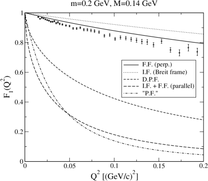
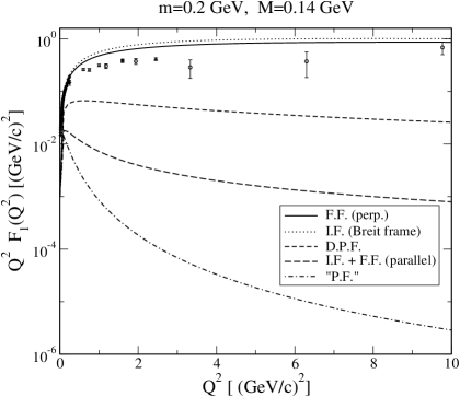
Figure 3: Pion charge form factor, $F_{1}(Q^{2})$, at small and high $Q^{2}$ (left and right panels respectively). In the latter case, the form factor is multiplied by $Q^{2}$ and represented on a logarithmic scale to emphasize the asymptotic behavior.

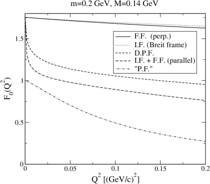
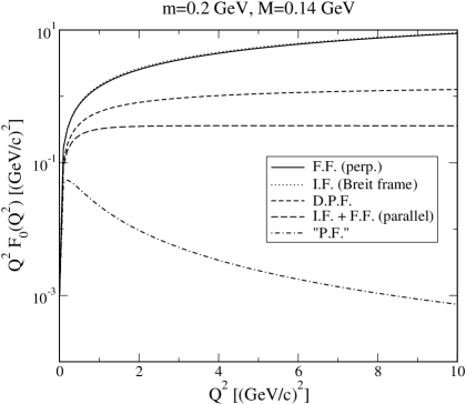
Figure 4: Same as for fig. 3 but for the scalar form factor $F_{0}(Q^{2})$.

We present in this section results for both the charge and scalar pion form factors calculated in the single-particle current approximation and for different RQM approaches. These ones include the instant and front forms with a standard momentum configuration, Breit frame in the former case (denoted I.F. (Breit frame)) and $q^{+}=0$ in the latter one (denoted F.F. (perp.)). Other frames are considered with a parallel momentum configuration (denoted I.F. + F.F. (parallel)). Results also include an approach inspired from Dirac’s point form (denoted D.P.F.) as well as an earlier “point form” that has been employed in previous works (denoted “P.F.”). Contrary to the other results, these ones are frame independent. As mentioned in sect. 3, expressions of form factors can be obtained by generalyzing those given elsewhere for the scalar-constituent case [28, 46].

Numerical results are shown altogether in figs. 3 and 4 for the charge and scalar form factors respectively. Two ranges of momentum transfers are considered in each case, low $Q^{2}$ on the l.h.s. ($0-0.2\,({\rm GeV/c})^{2})$ and high $Q^{2}$ on the r.h.s. ($0-10\,({\rm GeV/c})^{2}$). The first one is expected to evidence a sensitivity to the charge (or scalar) radius while the second one a priori emphasizes the asymptotic behavior. As this one should behave like $Q^{-2}$, the corresponding form factors are multiplied by $Q^{2}$ so that the product be close to a constant in the limit of large momentum transfers (up to log terms). Measurements for the charge form factor are also shown in fig. 3.

The comparison of different theoretical approaches evidences features quite similar to the scalar-constituent case [28]. The Breit-frame instant-form results slightly overshoot the front-form ones with $q^{+}=0$. The other instant- and front-form results with a parallel momentum configuration, which coincide with each other, show a fast drop off at small $Q^{2}$, a property that is also found for the point-form results. As explained elsewhere [22], this drop off points to a squared charge radius that is determined by the inverse of the squared pion mass and is larger than experiment by an order of magnitude. For a part, this sensitivity to the pion mass explains the large discrepancies between results shown at the r.h.s. of figs. 3 and 4, which roughly scale like in the scalar-constituent case.

The comparison with experiment, which is only possible for the charge form factor, shows that the standard instant- and front-form approaches provide reasonable results as a starting point while all the other ones are off, sometimes by orders of magnitude. This is again somewhat similar to the scalar-constituent case where the role of the experiment is played by an exact calculation. As has been suggested [28] and shown later on [46], the largest discrepancies point to a violation of Poincaré space-time translation invariance, which requires specific two-body currents to be restored. This does not necessary imply that the other results in the standard instant- and front-form approaches are fully under control.

Looking carefully at the corresponding product of the charge form factor with $Q^{2}$, shown at the r.h.s. of fig. 3 , it is found that the appearance of a plateau, which could suggest that the expected asymptotic behavior is reached, is misleading. The comparison with the scalar form factor, shown at the r.h.s. of fig. 4, is here very instructive. In this case, the same product increases, in agreement with possible log$(Q^{2})$ deviations and, moreover, is significantly larger. Globally, it thus appears that the above charge form factors at high $Q^{2}$ are suppressed with respect to the scalar ones, which can be better seen by examining results for much higher momentum transfers (see next section). The origin of the suppression, roughly given by a factor $Q^{2}$, resides for a part in the coupling of quarks to the external probe, as can be checked from considering matrix elements of the current between positive-energy spinors [22]. A similar suppression, but within a truncated field-theory light-front calculation, was mentioned in ref. [52]. This result represents an important difference with the scalar-particle case.

At this point, a few further remarks can be made. The spin-1/2 nature of the constituents also shows up in results at small $Q^{2}$. Its effect in the better cases (standard instant- and front-form approaches) is found to be very similar to the one produced by the Melosh transformation in other works [15], with an increased contribution to the charge radius (Darwin-Foldy term). Results evidence some sensitivity to the dynamics like the description of the confinement. This has not been considered in detail here but we notice that reproducing the pion-decay constant allows one to reduce the uncertainty.

5 Results with two-body currents and asymptotic behavior

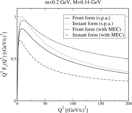
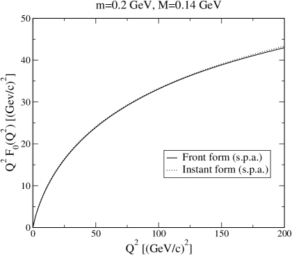
Figure 5: Form factors $F_{1}(Q^{2})$ and $F_{0}(Q^{2})$ in the ultra asymptotic domain: contribution from the single-particle current (s.p.a.) and, for $F_{1}(Q^{2})$, contribution incorporating two-body currents (with MEC). Calculations are performed in the standard instant and front-form approaches.

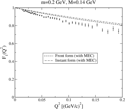
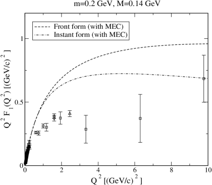
Figure 6: Effect of two-body currents on the charge form factor, $F_{1}(Q^{2})$, at low and intermediate momentum transfers: results are presented for the standard instant and front-form approaches.

We consider in this section the pion charge form factor with including the contribution of two-body currents. This is done for both the instant-form and front-form approaches, respectively in the standard Breit-frame and so-called $q^{+}=0$ configurations. As already mentioned, the other approaches suppose dominant contributions from specific two-body currents restoring the Poincaré space-time translation invariance. These ones could be determined along lines developed in ref. [46] but it is not clear how they will affect the contribution of two-body currents of interest here (possible double counting).

As two-body currents considered in this section are mainly motivated by the asymptotic behavior of the charge form factor, we first present results relevant to this feature. These ones, multiplied by $Q^{2}$, are given in fig. 5 (l.h.s.) for a range of $Q^{2}$ extending from 0 to 200 (GeV/c)². For the sake of the discussion, we also present in this figure (r.h.s.) results pertinent to the scalar form factor. The two-body currents also contribute at low and intermediate values of $Q^{2}$. The corresponding results for the charge form factor alone are shown in fig. 6. The range under consideration is the same as in fig. 3, but a linear scale instead of a logarithmic one is adopted for the r.h.s. part.

We first notice that, contrarily to what the consideration of the r.h.s. of fig. 3 would suggest, the asymptotic behavior of the charge form factor is not reached yet. Examination of fig. 5 (l.h.s.) clearly shows that the product of $Q^{2}$ with the charge form factor calculated from the single-particle current, after evidencing a maximum around $10$ (GeV/c)², begins to slowly decrease. The difference with the scalar form factor shown in the r.h.s. of the same figure, which has the right asymptotic behavior, is striking. Accounting for the contribution of two-body currents to the charge form factor allows one to obtain its asymptotic behavior which is expected to be given numerically by $F_{1}(Q^{2})_{Q^{2}\rightarrow\infty}=$ 0.17 (GeV/c)²$/Q^{2}$ for our pion description. As it can be seen on fig. 5 around $200$ (GeV/c)², this value is not far to be reached in the instant-form case but still rather far away in the front-form one. The different behavior can be explained as follows. The instant-form two-body current implies a contribution originating from the pseudo-scalar part of the interaction ($I^{-}_{ps}$), which cancels the single-particle one, leaving as a neat result the contribution due to the pseudo-axial vector part ($I^{-}_{pv}$), while this destructive contribution is absent in the front-form case. A few further comments may provide better insight on the above results. First, in spite of different formalisms, present results qualitatively agree with those of earlier works [8, 53]. Some of the quantitative differences, especially the onset of the asymptotic behavior at larger $Q^{2}$ in this work, can be related for a part to our pion description that involves sizeable high-momentum components. Second, the difference between the asymptotic value of the form factor given above in the text and the current one given by eq. (25), 0.11 (GeV/c)²$/Q^{2}$, can be ascribed to the non-perturbative effects mentioned in the comments about this last result (end of sect. 3.3).

Considering now the results for the charge form factor at very small transfers (l.h.s. of fig. 6), it is observed that the contribution of the two-body currents tends to remove the difference between the instant- and front-form form factors. Such a result is not totally unexpected as, for a part, the two-body currents tend to restore Lorentz invariance in first place and perhaps some Poincaré space-time translation invariance in second place. It actually holds for the contribution of the pseudo-scalar part of the interaction alone, $I^{-}_{ps}$ in eq. (LABEL:twobod2), what it should as the part related to the pseudo-axial vector part, $I^{-}_{pv}$, is irrelevant for the argument. It remains that some contribution could be due to the confinement interaction but its non-perturbative character does not allow one to determine how much it affects $I^{-}_{ps}$ in the instant form.

To some extent, the above Lorentz-invariance argument applies to the form factor in the intermediate range, shown in the r.h.s. of fig. 6, but the effect is larger than needed. We observe that the contribution of two-body currents tends to make the instant-form form factor closer to experiment while it makes the front-form one further away. To better understand the role of two-body currents depending on the form, it is useful to consider separately the two contributions in the instant form, $I^{-}_{ps}$ and $I^{-}_{pv}$, eq. (LABEL:twobod2). The first one, which has no well determined counterpart in the front-form case, is negative over the full range of $Q^{2}$ considered in this work and decreases faster than $Q^{-2}$. The second one, which is positive and provides the $Q^{-2}$ asymptotic behavior, is close to the contribution $I^{+}_{ps}+I^{+}_{pv}$ calculated in the front-form approach.

Having considered two-body currents, we can now discuss the pion charge radius to which they can contribute. This is done in relation with the expression $r^{2}_{\pi}=3/(4\,\pi^{2}\;f^{2}_{\pi})$, which gives the value $r^{2}_{\pi}=0.342\;{\rm fm}^{2}$ for $f_{\pi}=93$ MeV. A value that could be more relevant for the discussion is $r^{2}_{\pi}=0.263\;{\rm fm}^{2}$, which corresponds to $f_{\pi}=106$ MeV obtained with our pion description. In the instant form, it is expected that part of the contribution should have a counterpart in the piece of the two-body currents associated to the pseudo-scalar component, $I^{-}_{ps}$. We first notice that the squared matter radius has a relatively small role, of the order of $0.08\,{\rm fm}^{2}$ in the present calculation to be compared to the measured value of the squared charge radius, $0.43\,{\rm fm}^{2}$. We also notice that the part of two-body currents due to the pseudo-axial vector component of the interaction, also small ($-0.02\,{\rm fm}^{2}$), is irrelevant for a comparison with the above prediction which assumes a pseudo-scalar component and a point-like pion. As already mentioned, this approximate prediction should be compared to that part in our calculations which corresponds to the Darwin-Foldy term. Isolating this term in the instant-form results, we find $0.15\,{\rm fm}^{2}$ for the one-body current and $0.08\,{\rm fm}^{2}$ for the two-body one. The sum, $0.23\,{\rm fm}^{2}$, compares to the expectation $0.263\,{\rm fm}^{2}$. In the front form, where we only have a contribution from the one-body current, a similar procedure gives $0.29\,{\rm fm}^{2}$, which also compares to the expectation $0.263\,{\rm fm}^{2}$. Thus, there is a reasonable agreement of the present results for the charge radius and the approximate expectation advocated in many works. Another relation, suggested by the analysis of various contributions to the above expression of $r^{2}_{\pi}$, is worthwhile to be mentioned. The usual Darwin-Foldy correction to the form factor in the instant form takes the form $-Q^{2}/(8\,m_{q}^{2})$ (non-relativistic limit). When the similar term associated here to the two-body current is considered, one gets instead $-Q^{2}/(4\,m_{q}^{2})$. This last term can be seen as the first term in the $Q^{2}$ expansion of the vector-meson dominance model of form factors, $-Q^{2}/m_{V}^{2}$, where $m_{V}^{2}=4\,m_{q}^{2}+\cdots$.

When considering calculations of the two-body current contribution, a large sensitivity to various ingredients was found. Most of it points to the role of higher-order effects in the interaction which, for consistency, were neglected. These effects nevertheless show up in looking at some of the results presented here. As an example, it is likely that the charge and the scalar form factors in the asymptotic regime should be comparable, up to a factor 1-2. Examination of results presented in fig. 6 rather suggest that they differ by a factor 10-20. This can be largely explained by non-perturbative corrections to the wave function entering the calculation. Thus, these effects lead to log($Q^{2}/m_{q}^{2}$) terms that enhance the scalar form factor in the asymptotic domain while they are ignored in the present derivation of two-body currents based on a perturbative approach. An other hint about these non-perturbative effects is provided by the comparison of the contribution of two-body currents in different forms. While the contributions of the single-particle current in the standard instant- and front-form approaches are relatively close to each other, those for the two-body currents significantly differ. Most of the discrepancy can be traced back to the term $I^{-}_{ps}$, whose role exceeds the restoration of Lorentz invariance at soon as the momentum transfer increases.

6 Discussion and conclusion

We first considered in this work the single-particle contribution to the charge and pion form factors in different forms of RQM approaches. These ones include the standard instant and front forms (Breit frame and the momentum configuration $q^{+}=0$ respectively), the same forms with a “parallel” momentum configuration and the point form. The interaction entering the mass operator is chosen as the sum of a confining interaction and a gluon-exchange one, which is a priori essential for getting the right asymptotic behavior of form factors. For the case of the charge form factor, where measurements are available, the standard instant- and front-form approaches provide results relatively close to them. All the other results fall far apart, as a result of their dependence on the momentum transfer through the ratio $v=Q/(2\,M_{\pi})$. Thus the pattern evidenced by these results is very similar to that one obtained with a model of scalar particles [28]. As has been shown, the last results evidence a strong violation of Poincaré space-time translation invariance while this property is approximately fulfilled by the standard instant- and front-form ones. This discards the underlying approaches as efficient ones to describe the pion properties.

While there is some similarity of the above results with earlier ones for a theoretical model with scalar constituents, there are nevertheless differences. The most striking one concerns the ratio of the charge and scalar form factors. Whatever the approach, the first one is suppressed compared to the other one at high $Q^{2}$, preventing one from reproducing its expected asymptotic behavior, $Q^{-2}$. This result, which seems to characterize relativistic quantum mechanics approaches with a single-particle current, implies the spin-1/2 structure of the quarks. This conclusion is comforted by the consideration of the scalar form factor which, up to a finite coefficient, has the right power-law behavior.

We then looked at the two-body currents whose contributions are necessarily required to reproduce the asymptotic behavior of the charge pion form factor expected from QCD. This has been done in both the standard instant and front forms, which are the only approaches to provide a reasonable starting point for further improvement. The two-body currents have been derived on the basis that adding their contribution to that one generated by the wave function should allow one to recover the full Born amplitude. While the description of hadron properties at low- and high-momentum transfers are often considered as disconnected, we showed that the above two-body currents were able to reproduce the expected expression of the pion charge form factor in the asymptotic regime. This result involves the pseudo-vector pseudo-vector part of the Fierz-transformed one-gluon exchange interaction, in agreement with what is expected in field-theory based approaches [8]. Quantitatively, the relevance of this result appears at quite high momentum transfers, probably beyond the range where the pion charge form factor has been measured. At very low-momentum transfers, the contribution of these two-body currents depends on the form. While it increases the front-form form factor, as at high $Q^{2}$, it decreases the instant-form one. The total effect compares to the difference of the instant- and front-form results in the single-particle current approximation, which it tends to cancel. Such a result is expected for a part as far as the two-body currents we are considering should contribute to restore Lorentz invariance. Between the very low- and very high-$Q^{2}$ domain, it is difficult to attribute a specific role to the above two-body currents, but it does not seem to affect much the comparison with experiment.

We have not made any attempt to provide a better description of the measured pion charge form factor, being mainly concerned by the determination of an approach where the bulk contribution would be given by a one-body current so that the derivation of two-body currents of interest here be simplified as much as possible. Following refs. [16, 17], the introduction of some quark form factor could reduce the discrepancy with experiment. One can nevertheless guess that a smaller quark mass would contribute to get both a better value of $f_{\pi}$ and a better charge radius, hence a better form factor at very small $Q^{2}$. A pion description with a smaller amount of large momentum components could also have a similar effect. As, apart from the quark mass, the parameters entering the mass operator we used are essentially fixed, the only issue would be to modify the form of this operator. One can expect for instance that retardation effects, ignored here, could contribute to reduce the strength of the one-gluon exchange at short distances [39, 38] and, consequently, the interaction at high momenta. Thus, while relativistic quantum mechanics is not the most fundamental approach for describing the pion properties, getting these ones relatively well in this framework does not seem to be out of reach.

Acknowledgement
We are very grateful to O. Leitner for useful comments about recovering the asymptotic behavior of the pion charge form factor in the present approach.

Appendix A Accounting for the spin of the constituents in deriving the mass operator

The simplest expression of the RQM pion wave function reads;

$$\psi(p_{1},p_{2})\propto\bar{u}(p_{1})\gamma_{5}v(p_{2})\;\frac{m_{q}}{e_{k}}\;\phi_{0}(k),$$ (33)

where the variable $k$ is related to the constituent momenta by the relation $4\,e_{k}^{2}=(p_{1}+p_{2})^{2}$. The spinors are normalized as follows:

$$\sum_{spins}u(p)\bar{u}(p)=\frac{\gamma\cdot p+m_{q}}{2m_{q}},\;\;\;\sum_{spins}v(p)\bar{v}(p)=\frac{\gamma\cdot p-m_{q}}{2m_{q}}.$$ (34)

Other expressions of the pion wave function reduce to the above one, eq. (33), taking into account that the on-mass shell character of particles in the RQM framework allows one to use the Dirac equation for free particles. In principle, $\psi(p_{1},p_{2})$ is a solution of a wave equation which should be cast into the form of a mass operator equation by making some change of variable. The problem and the related constraints were considered for scalar particles, see ref. [27] for an example. When considering a standard meson-exchange interaction like the gluon one in the present case, the non-zero spin of constituents has to be accounted for, raising further problems. To illustrate them, it is instructive to look at the action of the spin part of this interaction together with that one for the pion wave function:

$$V\;\psi(p^{\prime}_{1},p^{\prime}_{2})\propto\sum_{spins}\bar{u}(p_{1})\gamma^{\mu}u(p^{\prime}_{1})\;\bar{v}(p^{\prime}_{2})\gamma_{\mu}v(p_{2})\;\bar{u}(p^{\prime}_{1})\gamma_{5}v(p^{\prime}_{2}).$$ (35)

Using a Fierz transformation, the spin part of the interaction can also be written:

$$\bar{u}(p_{1})\gamma^{\mu}u(p^{\prime}_{1})\;\bar{v}(p^{\prime}_{2})\gamma_{\mu}v(p_{2})=\bar{u}(p_{1})v(p_{2})\;\bar{v}(p^{\prime}_{2})u(p^{\prime}_{1})+\bar{u}(p_{1})i\gamma_{5}v(p_{2})\;\bar{v}(p^{\prime}_{2})i\gamma_{5}u(p^{\prime}_{1})$$

$$-\frac{1}{2}\bar{u}(p_{1})\gamma^{\mu}v(p_{2})\;\bar{v}(p^{\prime}_{2})\gamma_{\mu}u(p^{\prime}_{1})-\frac{1}{2}\bar{u}(p_{1})\gamma^{\mu}\gamma_{5}v(p_{2})\;\bar{v}(p^{\prime}_{2})\gamma_{\mu}\gamma_{5}u(p^{\prime}_{1}),$$ (36)

where one recognizes a term with the same structure as the input wave function ($\bar{u}\gamma_{5}v$) and another one with a pseudo-vector character ($\bar{u}\gamma_{\mu}\gamma_{5}v$). When performing the summation over spins in eq. (35), it is found that these two terms contribute, with the result:

$$\sum_{spins}\bar{u}(p_{1})\gamma^{\mu}u(p^{\prime}_{1})\;\bar{v}(p^{\prime}_{2})\gamma_{\mu}v(p_{2})\;\bar{u}(p^{\prime}_{1})\gamma_{5}v(p^{\prime}_{2})=$$

$$\hskip 56.9055pt\bar{u}(p_{1})\gamma_{5}v(p_{2})\;\frac{(p^{\prime}_{1}\cdot p^{\prime}_{2}+m_{q}^{2})}{m_{q}^{2}}-\frac{1}{2}\;\bar{u}(p_{1})\gamma^{\mu}\gamma_{5}v(p_{2})\;\frac{(p^{\prime}_{1}+p^{\prime}_{2})_{\mu}}{m_{q}}.$$ (37)

The first term at the r.h.s., where the dependence on variables relative to the initial and final states factorizes, does not provide any difficulty in reducing a wave equation to a mass operator. The second one does however. Writing $(p^{\prime}_{1}+p^{\prime}_{2})_{\mu}=(p^{\prime}_{1}+p^{\prime}_{2}-p_{1}-p_{2})_{\mu}+(p_{1}+p_{2})_{\mu}$ and using the Dirac equation, the above equation also reads:

$$\sum_{spins}\bar{u}(p_{1})\gamma^{\mu}u(p^{\prime}_{1})\;\bar{v}(p^{\prime}_{2})\gamma_{\mu}v(p_{2})\;\bar{u}(p^{\prime}_{1})\gamma_{5}v(p^{\prime}_{2})=$$

$$\hskip 56.9055pt\bar{u}(p_{1})\gamma_{5}v(p_{2})\;\frac{p^{\prime}_{1}\cdot p^{\prime}_{2}}{m_{q}^{2}}-\bar{u}(p_{1})\gamma^{\mu}\gamma_{5}v(p_{2})\;\frac{(p^{\prime}_{1}+p^{\prime}_{2}-p_{1}-p_{2})_{\mu}}{2\,m_{q}},$$ (38)

where the last term is seen to depend on the surface on which physics is described (through $\xi^{\mu}$), quite in the same way as a meson propagator would generally. The problem is well known in relativistic quantum mechanics. It points to the constraints that the interaction entering the mass operator has to fulfill. These ones implicitly account for higher-order corrections in the interaction, which cancel the above undesirable contributions. This is made possible by the fact that these contributions have an off-energy shell character (see eq. (4)). Discarding these ones, the relevant part of the gluon exchange appropriate for describing the pion in the RQM framework may thus be written in the following factorized form:

$$V\;\propto g^{2}\frac{\bar{u}(p_{1})i\gamma_{5}u(p_{2})\;\bar{v}(p^{\prime}_{2})i\gamma_{5}v(p^{\prime}_{1})}{(\vec{k}-\vec{k}^{\prime})^{2}}\;\Big{(}2-\frac{m^{2}_{q}\,(e^{2}_{k}+e^{2}_{k^{\prime}})}{2\,e^{2}_{k}\;e^{2}_{k^{\prime}}}\Big{)}\,.$$ (39)

The last factor has been introduced to represent as much as possible the effect of the factor $p^{\prime}_{1}\cdot p^{\prime}_{2}\;(=e^{2}_{k^{\prime}}+k^{\prime 2})$ in eq. (38), which originates from the original vector-vector nature of the interaction ($\gamma^{\mu}\;\gamma_{\mu}$), while keeping the symmetry between $k$ and $k^{\prime}$. It differs from the factor $(2-m_{q}^{2}/e^{2}_{k})^{1/2}(2-m_{q}^{2}/e^{2}_{k^{\prime}})^{1/2}$ introduced by Godfrey and Isgur [54] by off-energy shell corrections proportional to $m^{2}_{q}$, which are in any case part of the uncertainty on the derivation of the mass operator. Due to the presence of square root factors however, the last choice may introduce further complication in the derivation of two-body currents. Whatever the choice, we notice that a pseudo-scalar pseudo-scalar type interaction ($\gamma_{5}\;\gamma_{5}$) reproducing the non-relativistic limit of the one-gluon exchange would provide a different result (a factor $e^{2}_{k^{\prime}}$ instead of $e^{2}_{k^{\prime}}+k^{\prime 2}$ in the present case). Thus, the choice made here is consistent with the symmetry character of the interaction $V$, but could miss some off-shell corrections. Gathering all the relevant factors, the wave equation reads:

$$(M^{2}-4\,e_{k}^{2})\;\bar{u}(p_{1})\gamma_{5}v(p_{2})\;\frac{m_{q}}{e_{k}}\;\phi_{0}(k)=-\int\frac{d\vec{k}^{\prime}}{(2\,\pi)^{3}}\;\frac{4\;g^{2}\;\frac{4}{3}}{(\vec{k}-\vec{k}^{\prime})^{2}}\;\Big{(}2-\frac{m^{2}_{q}\,(e^{2}_{k}+e^{2}_{k^{\prime}})}{2\,e^{2}_{k}\;e^{2}_{k^{\prime}}}\Big{)}$$

$$\hskip 56.9055pt\times\frac{m_{q}^{2}}{\sqrt{e_{k}}\sqrt{e_{k^{\prime}}}}\bar{u}(p_{1})i\gamma_{5}v(p_{2})\;\;\frac{1}{2}\;\sum_{spins}\bar{v}(p^{\prime}_{2})i\gamma_{5}u(p^{\prime}_{1})\;\;\bar{u}(p^{\prime}_{1})\gamma_{5}v(p^{\prime}_{2})\;\frac{m_{q}}{e_{k^{\prime}}}\;\phi_{0}(k^{\prime})$$

$$\hskip 8.5359pt=-\int\frac{d\vec{k}^{\prime}}{(2\,\pi)^{3}}\;\frac{4\;g^{2}\;\frac{4}{3}}{(\vec{k}-\vec{k}^{\prime})^{2}}\;\frac{m_{q}^{2}}{\sqrt{e_{k}}\sqrt{e_{k^{\prime}}}}\;\bar{u}(p_{1})\gamma_{5}v(p_{2})\;\Big{(}2-\frac{m^{2}_{q}\,(e^{2}_{k}+e^{2}_{k^{\prime}})}{2\,e^{2}_{k}\;e^{2}_{k^{\prime}}}\Big{)}\frac{e_{k^{\prime}}^{2}}{m_{q}^{2}}\;\frac{m_{q}}{e_{k^{\prime}}}\;\phi_{0}(k^{\prime}),$$

(40)

which, after some simplification, is found to give eq. (1) (apart from the confinement part not considered here).

Appendix B High momentum behavior of solutions

The behavior of wave functions at high momenta, which in principle is relevant for calculating form factors in the asymptotic regime, is determined by the most singular part of the interaction. Examination of eq. (1) indicates that the problem relevant to the determination of this behavior amounts to look for solutions of the following equation:

$$(p-\frac{\alpha}{r})\;\tilde{\psi}(r)=0\,,$$ (41)

where $\tilde{\psi}(r)$ is the Fourier transform of the momentum wave function $\tilde{\phi}(k)=\sqrt{e_{k}}\;\phi_{0}(k)$ and $\alpha=8\,\alpha_{s}/3$. Though the problem was not always emphasized, it is part of earlier works [55, 54, 16]. Solutions can be obtained from the following relation:

$$p(r^{\mu-1})=\frac{\mu\;cotg(\frac{\mu\;\pi}{2})}{r}\;(r^{\mu-1})\,,$$ (42)

from which we infer that solutions in momentum space are given by:

$$\tilde{\psi}(p)\propto p^{-\mu-2}\,,$$ (43)

with $\alpha=\mu\;cotg(\frac{\mu\;\pi}{2})$. Particular cases are the following ones:

$$\alpha=\epsilon,\;\mu=1-\frac{2\,\epsilon}{\pi}:\;\;\;(p-\frac{\epsilon}{r})\;r^{\frac{2\,\epsilon}{\pi}}=0,\;\;\tilde{\psi}(p)\propto p^{-3+\frac{2\,\epsilon}{\pi}}\,,$$

$$\alpha=\frac{1}{2},\;\mu=1/2:\;\;\;(p-\frac{1}{2\,r})\;r^{-1/2}=0,\;\;\tilde{\psi}(p)\propto p^{-2.5}\,,$$

$$\alpha=\frac{2}{\pi},\;\mu=0:\;\;\;(p-\frac{2}{\pi\,r})\;r^{-1}=0,\;\;\tilde{\psi}(p)\propto p^{-2},({\rm limit\;case})\,.$$ (44)

The first case corresponds to a perturbative one which, in our case, implies the behavior $\tilde{\phi}(k)\propto k^{-3},\;\phi_{0}(k)\propto k^{-7/2}$. When the strength of the interaction increases, non-perturbative effects generally given by log terms can be large enough to change the asymptotic power, by half a unit for $\alpha=\frac{1}{2}$ and one unit for $\alpha=\frac{2}{\pi}$. As has been shown [36], the last case corresponds to the occurrence of a critical regime in the QED case. The relevance of this result for QCD and the spontaneous breaking of the chiral symmetry is not quite clear but we notice that the range for the strong coupling, $\alpha_{s}$, usually referred to is of the order or even exceeds the critical value of $\frac{2}{\pi}\simeq 0.64$ ($\alpha=1.33$ for $\alpha_{s}=0.5$). Possible problems related to the onset of a critical regime, that are generally ignored, appear here due to the quadratic form of the mass equation and the extra factor $\Big{(}2-(m^{2}_{q}\,(e^{2}_{k}+e^{2}_{k^{\prime}}))/(2\,e^{2}_{k}\;e^{2}_{k^{\prime}})\Big{)}$, which separately enhance the strength of the force by a factor 2 at large momentum. They could be alleviated by the decreasing of $\alpha_{s}$ with the momentum transfer, or the effect of retardation effects. In practice, we will choose a value of $\alpha_{s}$ that corresponds to $\alpha=0.5$ at most (i.e. $\alpha_{s}=3/16$).

Appendix C Two-body currents and asymptotic behavior

We consider in this appendix the derivation of two-body currents that are related to the one-gluon exchange and could contribute to the pion charge form factor in the asymptotic domain, of special interest in this work. This is done for the general case where physics is formulated on an arbitrary hyperplane of orientation $\xi^{\mu}$ and, for the following discussion, we introduce “positive” and “negative” energies as defined with respect to this orientation. Particular applications concern both the instant-form and the front-form approaches. Essentially, the derivation amounts to include contributions that are not accounted for in the single-particle contribution. This involves contributions with intermediate particles carrying a “negative” energy, which are not part of a RQM formalism. Contributions with a “positive” energy also occur but, in this case, they involve off-energy shell effects that the formalism ignores. These ones are not necessarily independent of the previous ones however. What corresponds to “negative”-energy components in a given approach often appears as an off-energy shell in another one.

Our starting point is the expression of the charge form factor given by eq. (13). In order to derive the two-body currents we look for, the relation with the Born amplitude shown in fig. 2 has to be established. This is done by demanding that they coincide for the contribution with a “positive” energy intermediate quark when higher orders in the interaction are discarded. We notice that the above procedure fixes the strength of the Born amplitude entering the calculation providing a check on the ability of the underlying formalism to account for it. The contribution to the form factor thus obtained reads:

$$\Delta F_{1}(Q^{2})=\int\frac{d\vec{p}_{i2}}{(2\,\pi)^{3}}\;\int\frac{d\vec{p}_{f2}}{(2\,\pi)^{3}}\;\;\frac{\xi\!\cdot\!(p_{i1}\!+\!p_{i2})}{2\,e_{i2}\;\;\xi\!\cdot\!p_{i1}}\;\Big{(}\frac{m_{q}}{e_{k_{i}}}\;\tilde{\phi}(k_{i})\Big{)}\;\frac{\xi\!\cdot\!I}{\xi\!\cdot\!(p_{i1}\!+\!p_{i2}\!+\!p_{f1}\!+\!p_{f2})}\hskip 14.22636pt$$

$$\times\;\frac{1}{\Big{(}m_{q}^{2}\!-\!p_{f}^{*2}\Big{)}}\;\frac{g^{2}\;\frac{4}{3}}{\mu^{2}\!-\!(p_{i2}\!-\!p_{f2})^{2}}\;\;\frac{\xi\!\cdot\!(p_{f1}\!+\!p_{f2})}{2\,e_{f2}\;\;\xi\!\cdot\!p_{f1}}\;\Big{(}\frac{m_{q}}{e_{k_{f}}}\;\tilde{\phi}(k_{f})\Big{)}+\;({\rm term:}\;i\leftrightarrow f)\,,$$ (45)

where $p^{*\,\mu}_{f}=P_{f}^{\mu}-p_{i2}^{\mu}$, while $I^{\mu}$ is given by:

$$I^{\mu} = \frac{1}{2}\;8\,m_{q}^{3}\;$$

$$\times\,{\rm Tr}\Bigg{[}\frac{m_{q}\!-\!\gamma\!\cdot\!p_{i2}}{2\,m}\,i\gamma_{5}\,\frac{m_{q}\!+\!\gamma\!\cdot\!p_{i1}}{2\,m_{q}}\;\gamma^{\mu}\;\frac{m_{q}\!+\!\gamma\!\cdot\!p^{*}_{f}}{2\,m_{q}}\;\gamma^{\nu}\;\frac{m_{q}\!+\!\gamma\!\cdot\!p_{f1}}{2\,m_{q}}\,i\gamma_{5}\,\frac{m_{q}\!-\!\gamma\!\cdot\!p_{f2}}{2\,m_{q}}\;\gamma_{\nu}\;\Bigg{]}$$

$$=2\,\frac{(m_{q}^{2}\!+\!p_{f1}\!\cdot\!p_{f2})}{m_{q}^{2}}\;\Bigg{[}\!p_{i1}\!\cdot\!p_{i2}\;p^{*\,\mu}_{f}-p_{i1}\!\cdot\!p^{*}_{f}\;p_{i2}^{\mu}+p_{i2}\!\cdot\!p^{*}_{f}\;p_{i1}^{\mu}+m_{q}^{2}\;(p^{*\,\mu}_{f}\!+\!p_{i1}^{\mu}\!+\!p_{i2}^{\mu})\Bigg{]}$$

$$-\Bigg{[}(p^{*}_{f}\cdot p_{f1}\!+\!p_{f2})\;(p_{i1}^{\mu}\!+\!p_{i2}^{\mu})+(p_{i1}\!+\!p_{i2}\cdot p_{f1}\!+\!p_{f2})\;p^{*\,\mu}_{f}-(p^{*}_{f}\cdot p_{i1}\!+\!p_{i2})\;(p_{f1}^{\mu}\!+\!p_{f2}^{\mu})$$

$$\;\;\;+(p_{i2}\cdot p_{f1}\!+\!p_{f2})\;p^{\mu}_{i1}-(p_{i1}\cdot p_{f1}\!+\!p_{f2})\;p^{\mu}_{i2}+p_{i1}\!\cdot\!p_{i2}\;(p_{f1}^{\mu}\!+\!p_{f2}^{\mu})+m^{2}\;(p_{f1}^{\mu}\!+\!p_{f2}^{\mu})\Bigg{]}\,.$$

In order to make the relation with the expression of the one-body current contribution to the form factor, eq. (13), the following points are noticed. The quark propagator can be written as the sum of two terms corresponding to “positive” and “negative” energies:

$$\frac{\gamma\!\cdot\!p^{*}+m_{q}}{m_{q}^{2}-p^{*\,2}}=\frac{\xi^{2}\;(\gamma\!\cdot\!\tilde{p}^{+}+m_{q})}{2\,\xi\!\cdot\!\tilde{p}^{+}\;(\xi\!\cdot\!\tilde{p}^{+}-\xi\!\cdot\!p^{*})}+\frac{\xi^{2}\;(\gamma\!\cdot\!\tilde{p}^{-}+m_{q})}{2\,\xi\!\cdot\!\tilde{p}^{-}\;(\xi\!\cdot\!\tilde{p}^{-}-\xi\!\cdot\!p^{*})}\,,$$ (47)

with

$$\tilde{p}^{+\,\mu}=p^{*\,\mu}-\xi^{\mu}\;\Bigg{(}\frac{\xi\!\cdot\!p^{*}-\xi\!\cdot\!\tilde{p}}{\xi^{2}}\Bigg{)},\;\;\;\;\;\;\;\;\tilde{p}^{-\,\mu}=p^{*\,\mu}-\xi^{\mu}\;\Bigg{(}\frac{\xi\!\cdot\!p^{*}+\xi\!\cdot\!\tilde{p}}{\xi^{2}}\Bigg{)}\,,$$

$$\xi\!\cdot\!\tilde{p}=\sqrt{(\xi\!\cdot\!p^{*})^{2}+\xi^{2}\;(m_{q}^{2}\!-\!p^{*\,2})}=\xi\!\cdot\!\tilde{p}^{+}=-\xi\!\cdot\!\tilde{p}^{-},\;\;\;\;\;\;\;\;\tilde{p}^{+\,2}=\tilde{p}^{-\,2}=m_{q}^{2}\,.$$ (48)

Of course, contributions corresponding to a “negative” energy or to the part of the interaction with a pseudo-vector character, which cannot be accounted for in a RQM formalism and give rise to the two-body currents we looked for, are discarded at this point. Now, some replacements, which are justified by the lowest-order interaction terms of interest here, have to be made:

$$\frac{g^{2}\;\frac{4}{3}}{\mu^{2}-(p_{i2}\!-\!p_{f2})^{2}}\hskip 28.45274pt\rightarrow\frac{g_{eff}^{2}\;\frac{4}{3}}{\mu^{2}+(\vec{k}_{f}-\vec{\tilde{k}}_{f})^{2}}\,,$$

$$\frac{\xi^{2}}{(\xi\!\cdot\!\tilde{p}_{f}^{+}-\xi\!\cdot\!p^{*})}\hskip 39.83385pt\rightarrow\frac{2\,\xi\!\cdot\!(\tilde{p}_{f}^{+}\!+\!p_{i2})}{(\tilde{p}_{f}^{+}+p_{i2})^{2}-M^{2}}\,,$$

$$2\,\frac{(m_{q}^{2}\!+\!p_{f1}\!\cdot\!p_{f2})}{m_{q}^{2}}\hskip 28.45274pt\rightarrow\frac{(p_{i2}\!+\!\tilde{p}^{+}_{f})\!\cdot\!(p_{f1}\!+\!p_{f2})}{m_{q}^{2}\!+\!\tilde{p}^{+}_{f}\!\cdot\!p_{i2}}+\Big{(}4\,\frac{e^{2}_{k_{f}}}{m_{q}^{2}}-\frac{e^{2}_{k_{f}}+e^{2}_{\tilde{k}_{f}}}{e^{2}_{\tilde{k}_{f}}}\Big{)}\,.$$ (49)

Apart from the first term at the r.h.s. of the last expression, which will be included in two-body currents associated with a “positive” energy intermediate state, the above replacements allow one to consider the integration over $\vec{p}_{f2}$ in eq. (45). After adding the confining interaction, which has no direct role on the asymptotic behavior, one can use eq. (1 ) and then recovers the wave function $\tilde{\phi}(\tilde{k}_{f})$. The identity with the expression of the form factor, $F_{1}^{(1)}(Q^{2})$, eq. (13), is finally obtained by making the change of notations: $p_{i2}\rightarrow p$, $p_{i1}\rightarrow p_{i}$, $\tilde{p}_{f}^{+}\rightarrow p_{f}$, $\tilde{k}_{f}\rightarrow k_{f}$.

The expression of two-body currents, which correspond to the terms discarded above, can now be obtained:

$$F^{(2)}_{1}(Q^{2})=\int\frac{d\vec{p}_{i2}}{(2\,\pi)^{3}}\;\;\int\frac{d\vec{p}_{f2}}{(2\,\pi)^{3}}\;\;\frac{\xi\!\cdot\!(p_{i1}\!+\!p_{i2})}{2\,e_{i2}\;\;\xi\!\cdot\!p_{i1}}\;\Big{(}\frac{m_{q}}{e_{k_{i}}}\;\tilde{\phi}(k_{i})\Big{)}\;\frac{\xi\!\cdot\!(p_{f1}\!+\!p_{f2})}{2\,e_{f2}\;\;\xi\!\cdot\!p_{f1}}\;\Big{(}\frac{m_{q}}{e_{k_{f}}}\;\tilde{\phi}(k_{f})\Big{)}$$

$$\times\frac{g^{2}\;\frac{4}{3}}{\mu^{2}-(p_{i2}-p_{f2})^{2}}\;\Big{(}I^{-}_{ps}+I^{-}_{pv}+I^{+}_{ps}+I^{+}_{pv}\Big{)}+\;({\rm term:}\;i\leftrightarrow f)\,,$$ (50)

where:

$$I^{-}_{ps}=\frac{\xi^{2}}{\xi\!\cdot\!(p_{i1}+p_{f1}+p_{i2}+p_{f2})\;\;2\,\xi\!\cdot\!\tilde{p}_{f}\;(\xi\!\cdot\!\tilde{p}_{f}+\xi\!\cdot\!(P_{f}\!-\!p_{i2}))}\;$$

$$\times\,2\,\frac{m_{q}^{2}\!+\!p_{f1}\!\cdot\!p_{f2}}{m_{q}^{2}}\Bigg{[}p_{i1}\!\cdot\!p_{i2}\;\xi\!\cdot\!\tilde{p}^{-}_{f}-p_{i1}\!\cdot\!\tilde{p}^{-}_{f}\;\xi\!\cdot\!p_{i2}+p_{i2}\!\cdot\!\tilde{p}^{-}_{f}\;\xi\!\cdot\!p_{i1}+m_{q}^{2}\,\xi\!\cdot\!(\tilde{p}^{-}_{f}\!+\!p_{i1}\!+\!p_{i2})\Bigg{]}\,,$$

$$I^{-}_{pv}=-\frac{\xi^{2}}{\xi\!\cdot\!(p_{i1}+p_{f1}+p_{i2}+p_{f2})\;\;2\,\xi\!\cdot\!\tilde{p}_{f}\;(\xi\!\cdot\!\tilde{p}_{f}+\xi\!\cdot\!(P_{f}\!-\!p_{i2}))}\;$$

$$\times\Bigg{[}\tilde{p}^{-}_{f}\!\cdot\!(p_{f1}\!+\!p_{f2})\;\xi\!\cdot\!(p_{i1}\!+\!p_{i2})+(p_{i1}\!+\!p_{i2})\!\cdot\!(p_{f1}\!+\!p_{f2})\;\xi\!\cdot\!\tilde{p}^{-}_{f}-\tilde{p}^{-}_{f}\!\cdot\!(p_{i1}\!+\!p_{i2})\;\xi\!\cdot\!(p_{f1}\!+\!p_{f2})$$

$$\;\;\;+p_{i2}\!\cdot\!(p_{f1}\!+\!p_{f2})\;\xi\!\cdot\!p_{i1}-p_{i1}\!\cdot\!(p_{f1}\!+\!p_{f2})\;\xi\!\cdot\!p_{i2}+(m_{q}^{2}+p_{i1}\!\cdot\!p_{i2})\;\xi\!\cdot\!(p_{f1}\!+\!p_{f2})\Bigg{]}\,,$$

$$I^{+}_{ps}+I^{+}_{pv}=\frac{\xi^{2}}{\xi\!\cdot\!(p_{i1}+p_{f1}+p_{i2}+p_{f2})\;\;2\,\xi\!\cdot\!\tilde{p}_{f}\;(\xi\!\cdot\!\tilde{p}_{f}-\xi\!\cdot\!(P_{f}\!-\!p_{i2}))}\;$$

$$\times\Bigg{[}\frac{(p_{i2}\!+\!\tilde{p}^{+}_{f})\!\cdot\!(p_{f1}\!+\!p_{f2})}{m_{q}^{2}\!+\!\tilde{p}^{+}_{f}\!\cdot\!p_{i2}}\,\Big{(}p_{i1}\!\cdot\!p_{i2}\;\xi\!\cdot\!\tilde{p}^{+}_{f}-p_{i1}\!\cdot\!\tilde{p}^{+}_{f}\;\xi\!\cdot\!p_{i2}+p_{i2}\!\cdot\!\tilde{p}^{+}_{f}\;\xi\!\cdot\!p_{i1}+m_{q}^{2}\,\xi\!\cdot\!(\tilde{p}^{+}_{f}\!+\!p_{i1}\!+\!p_{i2})\Big{)}$$

$$-\Big{(}\tilde{p}^{+}_{f}\!\cdot\!(p_{f1}\!+\!p_{f2})\;\xi\!\cdot\!(p_{i1}\!+\!p_{i2})+(p_{i1}\!+\!p_{i2})\!\cdot\!(p_{f1}\!+\!p_{f2})\;\xi\!\cdot\!\tilde{p}^{+}_{f}-\tilde{p}^{+}_{f}\!\cdot\!(p_{i1}\!+\!p_{i2})\;\xi\!\cdot\!(p_{f1}\!+\!p_{f2})$$

$$\;\;\;+p_{i2}\!\cdot\!(p_{f1}\!+\!p_{f2})\;\xi\!\cdot\!p_{i1}-p_{i1}\!\cdot\!(p_{f1}\!+\!p_{f2})\;\xi\!\cdot\!p_{i2}+(m_{q}^{2}+p_{i1}\!\cdot\!p_{i2})\;\xi\!\cdot\!(p_{f1}\!+\!p_{f2})\Big{)}\Bigg{]}$$

$$+\frac{\xi^{2}}{2\,\xi\!\cdot\!\tilde{p}_{f}}\;\Bigg{[}\frac{1}{\xi\!\cdot\!(p_{i1}+p_{f1}+p_{i2}+p_{f2})\;\;(\xi\!\cdot\!\tilde{p}_{f}-\xi\!\cdot\!(P_{f}\!-\!p_{i2})}$$

$$\hskip 56.9055pt-\frac{1}{\xi\!\cdot\!(p_{i1}+\tilde{p}_{f}+2\,p_{i2})}\;\;\Bigg{(}\frac{1}{\xi\!\cdot\!(\tilde{p}_{f}+p_{i2})-\xi\!\cdot\!P_{f}}+\frac{1}{\xi\!\cdot\!(\tilde{p}_{f}+p_{i2})+\xi\!\cdot\!P_{f}}\Bigg{)}\Bigg{]}$$

$$\hskip 28.45274pt\times\Bigg{[}\Bigg{(}2\,\frac{m_{q}^{2}\!+\!p_{f1}\!\cdot\!p_{f2}}{m_{q}^{2}}-\frac{(m_{q}^{2}\!+\!p_{i2}\!\cdot\!\tilde{p}^{+}_{f}))+(m_{q}^{2}\!+\!p_{f1}\!\cdot\!p_{f2})}{m_{q}^{2}\!+\!\tilde{p}^{+}_{f}\!\cdot\!p_{i2}}\Bigg{)}$$

$$\hskip 56.9055pt\times\Big{(}p_{i1}\!\cdot\!p_{i2}\;\xi\!\cdot\!\tilde{p}^{+}_{f}-p_{i1}\!\cdot\!\tilde{p}^{+}_{f}\;\xi\!\cdot\!p_{i2}+p_{i2}\!\cdot\!\tilde{p}^{+}_{f}\;\xi\!\cdot\!p_{i1}+m_{q}^{2}\,\xi\!\cdot\!(\tilde{p}^{+}_{f}\!+\!p_{i1}\!+\!p_{i2})\Big{)}\Bigg{]}\,.$$ (51)

Examination of the denominator of $I^{-}$ shows the presence of a factor, $\xi\!\cdot\!\tilde{p}_{f}+\xi\!\cdot\!(P_{f}\!-\!p_{i2})$, which has no support in time-ordered diagrams, as can be seen in schematic models with scalar particles. It is cancelled by another term with the result to be replaced by $\tilde{p}_{f}+p_{i1}+\xi\!\cdot\!(P_{f}\!-\!P_{i})$, which amounts to taking into account off-energy shell corrections. This has the advantage of removing a contribution that has a singular behavior in the limit of a massless pion (instant-form case). Thus, a more elaborate and less sensitive expression for $I^{-}_{ps}$ and $I^{-}_{pv}$, which we will use, is the following:

$$I^{-}_{ps}=\frac{\xi^{2}}{\xi\!\cdot\!(p_{i1}+p_{f1}+p_{i2}+p_{f2})\;\;2\,\xi\!\cdot\!\tilde{p}_{f}\;\Big{(}\xi\!\cdot\!(\tilde{p}_{f}+p_{i1})+\xi\!\cdot\!(P_{f}\!-\!P_{i})\Big{)}}\;$$

$$\times 2\,\frac{m_{q}^{2}\!+\!p_{f1}\!\cdot\!p_{f2}}{m_{q}^{2}}\Bigg{[}p_{i1}\!\cdot\!p_{i2}\;\xi\!\cdot\!\tilde{p}^{-}_{f}-p_{i1}\!\cdot\!\tilde{p}^{-}_{f}\;\xi\!\cdot\!p_{i2}+p_{i2}\!\cdot\!\tilde{p}^{-}_{f}\;\xi\!\cdot\!p_{i1}+m_{q}^{2}\,\xi\!\cdot\!(\tilde{p}^{-}_{f}\!+\!p_{i1}\!+\!p_{i2})\Bigg{]}\,,$$

$$I^{-}_{pv}=-\frac{\xi^{2}}{\xi\!\cdot\!(p_{i1}+p_{f1}+p_{i2}+p_{f2})\;\;2\,\xi\!\cdot\!\tilde{p}_{f}\;(\xi\!\cdot\!(\tilde{p}_{f}+p_{i1})+\xi\!\cdot\!(P_{f}\!-\!P_{i}))}\;$$

$$\times\Bigg{[}\tilde{p}^{-}_{f}\!\cdot\!(p_{f1}\!+\!p_{f2})\;\xi\!\cdot\!(p_{i1}\!+\!p_{i2})+(p_{i1}\!+\!p_{i2})\!\cdot\!(p_{f1}\!+\!p_{f2})\;\xi\!\cdot\!\tilde{p}^{-}_{f}-\tilde{p}^{-}_{f}\!\cdot\!(p_{i1}\!+\!p_{i2})\;\xi\!\cdot\!(p_{f1}\!+\!p_{f2})$$

$$\;\;\;+p_{i2}\!\cdot\!(p_{f1}\!+\!p_{f2})\;\xi\!\cdot\!p_{i1}-p_{i1}\!\cdot\!(p_{f1}\!+\!p_{f2})\;\xi\!\cdot\!p_{i2}+(m_{q}^{2}+p_{i1}\!\cdot\!p_{i2})\;\xi\!\cdot\!(p_{f1}\!+\!p_{f2})\Bigg{]}\,.$$ (52)

In the instant-form approach, and for the Breit frame, the above contribution does not show any explicit dependence on the pion mass. In the front-form approach, it vanishes due to the presence of the factor $\xi^{2}$.

The expression for $I^{+}_{ps}+I^{+}_{pv}$ can also be transformed. The factor at the denominator, $\xi\!\cdot\!\tilde{p}_{f}-\xi\!\cdot\!(P_{f}\!-\!p_{i2})$, can be replaced by $\xi\!\cdot\!(\tilde{p}_{f}+p_{i2}-p_{f1}-p_{f2})$, which again amounts to neglect off-energy shell corrections. This term may be more singular but it turns out that the numerator vanishes at the same time. Some simplification can therefore be made. Moreover, the whole quantity goes to zero with the momentum transfer, allowing to factorize the term $\tilde{p}^{+}_{f}\!-\!p_{i1}$. The resulting expression we will use is thus:

$$I^{+}_{ps}+I^{+}_{pv} = -\frac{1}{\xi\!\cdot\!(p_{i1}+p_{f1}+p_{i2}+p_{f2})\;\;2\,\xi\!\cdot\!\tilde{p}_{f}\;(m_{q}^{2}\!+\!\tilde{p}^{+}_{f}\!\cdot\!p_{i2})}\;$$

$$\times\Bigg{[}\xi\!\cdot\!\tilde{p}^{+}_{f}\;\;\Big{(}(\tilde{p}^{+}_{f}\!-\!p_{i1})\!\cdot\!\xi\;\;(m_{q}^{2}\!+\!p_{i1}\!\cdot\!p_{i2})-(p_{i1}\!+\!p_{i2})\!\cdot\!\xi\;\;(\tilde{p}^{+}_{f}\!-\!p_{i1})\!\cdot\!p_{i2}\Big{)}$$

$$-(\tilde{p}^{+}_{f}\!+\!p_{i2})\!\cdot\!\xi\;\;p_{i2}\!\cdot\!\xi\;\;(\tilde{p}^{+}_{f}\!-\!p_{i1})\!\cdot\!p_{i1}$$

$$+\Big{(}(\tilde{p}^{+}_{f}\!-\!p_{i1})\!\cdot\!(p_{i1}\!+\!p_{i2})\;\xi^{2}-(\tilde{p}^{+}_{f}\!-\!p_{i1})\!\cdot\!\xi\;\;p_{i2}\!\cdot\!\xi\Big{)}\;(m_{q}^{2}\!+\!\tilde{p}^{+}_{f}\!\cdot\!p_{i2})\Bigg{]}$$

$$+\frac{\xi^{2}\;(\tilde{p}^{+}_{f}\!-\!p_{i1})\!\cdot\!\xi}{\xi\!\cdot\!(p_{i1}+p_{f1}+p_{i2}+p_{f2})\;\;2\,\xi\!\cdot\!\tilde{p}_{f}\;\xi\!\cdot\!(p_{i1}+\tilde{p}_{f}+2\,p_{i2})\;\xi\!\cdot\!(p_{i2}+\tilde{p}_{f}+p_{f1}+p_{f2})}$$

$$\times\Bigg{[}\Bigg{(}2\,\frac{m_{q}^{2}\!+\!p_{f1}\!\cdot\!p_{f2}}{m_{q}^{2}}-\frac{(m_{q}^{2}\!+\!p_{i2}\!\cdot\!\tilde{p}^{+}_{f}))+(m_{q}^{2}\!+\!p_{f1}\!\cdot\!p_{f2})}{m_{q}^{2}\!+\!\tilde{p}^{+}_{f}\!\cdot\!p_{i2}}\Bigg{)}$$

$$\hskip 28.45274pt\times\Big{(}p_{i1}\!\cdot\!p_{i2}\;\xi\!\cdot\!\tilde{p}^{+}_{f}-p_{i1}\!\cdot\!\tilde{p}^{+}_{f}\;\xi\!\cdot\!p_{i2}+p_{i2}\!\cdot\!\tilde{p}^{+}_{f}\;\xi\!\cdot\!p_{i1}+m_{q}^{2}\,\xi\!\cdot\!(\tilde{p}^{+}_{f}\!+\!p_{i1}\!+\!p_{i2})\Big{)}\Bigg{]}\,.$$

It can be checked that the above expression vanishes for both the instant form and the Breit frame ($\vec{P}_{f}=-\vec{P}_{i}$). It does not however away from this configuration. In the configuration $E_{i}=E_{f}$ together with the limit $|\vec{P}_{i}+\vec{P}_{i}|\rightarrow\infty$, the expression is found to be identical to the usual front-form one ($q^{+}=0$). This one could be obtained from the above one using standard changes of variable.

The derivation of two-body currents considered in this appendix could be easily extended to the Lorentz-scalar form factor. As this one already evidences the expected asymptotic power law, except perhaps for a numerical factor, the need for considering two-body currents is not as strong as for the charge form factor. Moreover, a perturbative calculation may reveal to provide little effect in the $Q^{2}$ domain where it does for the other form factor.

References

- [1] C. J. Bebek et al., Phys. Rev. D 17, 1693 (1978).
- [2] S. R. Amendolia et al., Nucl. Phys. B 277, 168 (1986).
- [3] J. Volmer et al., Phys. Rev. Lett. 86, 1713 (2001).
- [4] T. Horn et al., Phys. Rev. Lett. 97, 192001 (2006).
- [5] V. Tadevosyan et al., Phys. Rev. C 75, 055205 (2007).
- [6] G. M. Huber et al., nucl-ex/0809.3052.
- [7] C. D. Roberts, Nucl. Phys. A 605, 475 (1996).
- [8] P. Maris, C. D. Roberts, Phys. Rev. C 58, 3659 (1998).
- [9] P. Maris, P. C. Tandy, Phys. Rev. C 62, 055204 (2000).
- [10] D. Merten, et al., Eur. Phys. J. A 14, 477 (2002).
- [11] S. Simula, Phys. Rev. C 66, 035201 (2002).
- [12] B. Bakker, H.-M. Choi, C.-R. Ji, Phys. Rev. D 63, 074014 (2001).
- [13] J. P. B. C. de Melo et al., Nucl. Phys. A 707, 399 (2002).
- [14] N. Isgur, C. H. Llewellyn Smith, Phys. Rev. Lett. 52, 1080 (1984).
- [15] P. L. Chung, F. Coester, W. N. Polyzou, Phys. Lett. B 205, 545 (1988).
- [16] F. Cardarelli et al., Phys. Lett. B 332, 1 (1994).
- [17] F. Cardarelli, E. Pace, G. Salmé, S. Simula, Phys. Lett. B 357, 267 (1995).
- [18] H.-M. Choi, C.-R. Ji, Phys. Rev. D 59, 074015 (1999).
- [19] J. P. C. B. de Melo, H. W. L. Naus, T. Frederico, Phys. Rev. C 59, 2278 (1999).
- [20] T. W. Allen, W. H. Klink, Phys. Rev. C 58, 3670 (1998).
- [21] A. F. Krutov, V. E. Troitsky, Phys. Rev. C 65, 045501 (2002).
- [22] A. Amghar, B. Desplanques and L. Theußl, Phys. Lett. B 574, 201 (2003).
- [23] F. Coester, W. N. Polyzou, nucl-th/0405082.
- [24] Jun He, B. Julia-Diaz, Yu-bing Dong, Phys. Lett. B 602, 212 (2004).
- [25] Q. B. Li, D. O. Riska, Phys. Rev. C 77, 045207 (2008).
- [26] P. A. M. Dirac, Rev. Mod. Phys. 21, 392 (1949).
- [27] A. Amghar, B. Desplanques, L. Theußl, Nucl. Phys. A 714, 213 (2003).
- [28] B. Desplanques, preprint, nucl-th/0407074.
- [29] S. J. Brodsky, G. R. Farrar, Phys. Rev. D 11, 1309 (1975).
- [30] G. R. Farrar, D. R. Jackson, Phys. Rev. Lett. 43, 246 (1979).
- [31] G. P. Lepage, S. J. Brodsky, Phys. Lett. B 87, 359 (1979).
- [32] B. Desplanques, L. Theußl, Eur. Phys. J. A 13, 461 (2002).
- [33] B. Desplanques and L. Theußl, Eur. Phys. J. A 21, 93 (2004).
- [34] B. Desplanques, in NSTAR2004, eds. J.P. Bocquet, V. Kuznetsov, D. Rebreyend, World Scientific (nucl-th/0405060).
- [35] J. L. Basdevant and S. Boukraa, Z. Phys. C 30, 103 (1986).
- [36] A. Le Youanc, L. Oliver, J. C. Raynal, J. Math. Phys. 38, 3997 (1997).
- [37] C. Alabiso, G. Schierholz, Phys. Rev. D 10, 960 (1974).
- [38] A. Amghar, B. Desplanques, L. Theußl, Nucl. Phys. A 694, 439 (2001).
- [39] A. Amghar, B. Desplanques, Few-Body Syst. 28, 65 (2000).
- [40] B. Desplanques, B. Silvestre-Brac, F. Cano, P. Gonzalez and S. Noguera, Few-Body Syst. 29, 169 (2000).
- [41] B. Bakamjian, L. H. Thomas, Phys. Rev. 92, 1300 (1953).
- [42] B. Desplanques, Nucl. Phys. A 748, 139 (2005).
- [43] B. Bakamjian, Phys. Rev. 121, 1849 (1961).
- [44] S. N. Sokolov, Theor. Math. Phys. 62, 140 (1985).
- [45] W. H. Klink, Phys. Rev. C 58, 3587 (1998).
- [46] B. Desplanques and Y.B. Dong, Eur. Phys. J. A 37, 33 (2008).
- [47] B. Desplanques, L. Theußl, S. Noguera, Phys. Rev. C 65, 038202 (2002).
- [48] A. V. Efrimov and A. V. Radyushkin, Phys. Lett. B 94, 245 (1980).
- [49] R. Tarrach, Z. Phys. C 2, 221 (1979).
- [50] S. B. Gerasimov, Yad. Fiz. 29, 513 (1979).
- [51] V. Bernard, U. Meisner, Phys. Rev. Lett. 61, 2296 (1988).
- [52] J. Carbonell, B. Desplanques, V. A. Karmanov, J.-F. Mathiot, Phys. Reports 300, 215 (1998).
- [53] V. Braguta, W. Lucha, D. Melikhov, Phys. Lett. B 661, 354 (2008).
- [54] S. Godfrey, N. Isgur, Phys. Rev. D 32, 189 (1985).
- [55] J. Carlson, J. B. Kogut, V. R. Pandharipande, Phys. Rev. D 28, 2807 (1983).