Nonlinear effect on the transmission of light in a cavity array

Abstract

Taking nonlinear effect into account, we study theoretically the transmission properties of photons in a one-dimensional coupled cavities, the cavity located at the center of the cavity array is coupled to a two-level system. By the traditional scattering theory, we calculate the transmission rate of photons along the cavities, and discuss the effect of nonlinearity on the photon transport. The results show that the controllable two-level system can act as a quantum switch in the coherent transport of photons. The dynamics of such a system is also studied by numerical simulations, the effect of the atom-field detuning and nonlinearity on the dynamics is shown and discussed.

I Introduction

Recent experimental progress in the fabrication of microcavity arrays and the realization of the quantum regime in the coupling of atomic-like structures to quantized electromagnetic modes inside the cavities armani03 ; aoki06 ; barclay06 ; akahane03 ; hennessy07 ; wallraff04 ; trupke07 ; colombe07 open up the possibility of using them as quantum simulators of many-body physics. The possibility to create such cavity arrays have stimulated a number of theoretical investigations on the transport physicsfan05 ; sun08 ; xu00 , with particular emphasis on possible analogies with mesoscopic phenomena in the electronic context. This study is motivated by the preparation of new quantum states for photons or combined photonic-atomic excitations, which offer advantages over other systems for the realization of strongly interacting many-body models in quantum optical systems. For Josephson junction arrays and optical lattices, it is difficult to address individual sites due to the small separations between neighboring sites, but this is easy for coupled cavity arrays due to the large separations which are usually dozens of micrometers and can therefore be accurately accessed by optical frequencies.

Coupled cavity arrays have several interesting potential applications, including quantum information processing and simulations of quantum strongly correlated many-body systems. By using a real-space model Hamiltonian, it has been shown that the transmission of a single photon can be switched on or off in one-dimensional waveguide coupled with superconductivity quantum bitsfan05 . Indeed the transmission can be switched to any predicted value with a tiny change in the magnetic field when the sharper Fano resonance peak is employed. For a single photon inside a one-dimensional resonator waveguide with a two-level system, a general spectral structure in which the reflection and transmission beyond the usual Breit-Wigner and Fano line shapes is predictedsun08 . The atom in a half-waveguide can play an intrinsic role of semi-transparent mirror for the single photon, leading the system to be flexible under control.

Nonlinearity may appear in quantum systems due to the many-body effects and/or system-environment couplings. Transport and tunneling properties of nonlinear system (for example, Bose-Einstein condensates) are of considerable current interests, both experimentally and theoretically. Quantum tunneling through a barrier is a paradigm of quantum mechanics and usually takes place on a nanoscopic scale, such as in two supperconductors separated by a thin insulatorlikharev79 and two reservoirs of superfluid helium connected by nanoscopic aperturespereverzev97 ; sukhatme01 . Recently, tunneling on a macroscopic scale ($\mu m$) in two weakly linked Bose-Einstein condensates in a double-well potential has been observedalbiez05 . Similar to tunneling oscillations in superconducting and superfluid Josephson junctions, Josephson oscillations are observed when the initial population difference is chosen to be below a critical value. When the initial population difference exceeds the critical value, an interesting feature can be observed, i.e., tunneling oscillations are suppressed due to the nonlinear condensate self-interactions. This phenomenon is known as the macroscopic quantum self-trapping.

Here we explore a different regime of transport for photons in a cavity array coupled to a two-level system. Nonlinear effects arising from Kerr medium in cavities are taken into account. The paper is organized as follows. In Sec.II, we present a general formulism for the atom-cavity array. By the traditional scattering theory, the transmission rate is calculated and discussed in Sec. III. In Sec. IV, we present a numerical simulation for the dynamics of the coupled atom-cavity array system. An experimentally realizable proposal to observe the prediction is suggested in Sec.V. Finally, we conclude our results in Sec.VI.

II Formulism

Consider a cavity array coupling to a two-level system. Photon hopping can occur between neighboring cavities due to the overlap of the special profile of the cavity modes, see figure 1.

Figure 1: (color online)Schematic illustration of the coupled cavity arrays, in which the photons propagate. A two-level atom is located at the zeroth cavity and coupled to the cavity field.

Introducing the creation and annihilation operators of the cavity modes, $a_{j}^{\dagger}$ and $a_{j}$, the Hamiltonian of the field in the cavity can be written as,

$$H_{c}^{l}=\omega\sum_{j}a_{j}^{{\dagger}}a_{j}-\xi\Sigma_{j}(a_{j}^{{\dagger}}a_{j+1}+h.c.).$$ (1)

In Hamiltonian Eq.(1) that all the cavities have the same resonant frequency and the same spacing overlap between all neighboring cavities have been assumed. In contrast to the previous studies, we focus here on the influence of nonlinearity on the transparent properties of photons in the cavity array. The nonlinearity comes from the optical Kerr effects, where the electronic field is due to the light itself. Taking this nonlinearity into account, we add an additional term $g\sum_{j}(a^{\dagger}a)^{2}$ into the Hamiltonian, and the Hamiltonian for the cavity array therefore becomes

$$H_{c}=H_{c}^{l}+g\sum_{j}(a_{j}^{{\dagger}}a_{j})^{2}.$$ (2)

The location of the two-level atom in the cavity array is chosen to be the origin of the coordinate axis, which is only coupled to the zeroth cavity field in the cavity array. We assume that the cavity decay and atomic spontaneous emission are ignored. This configuration is different from that in Refszhou07 ; hu07 ; hartmann06 ; rakhmanov08 , where several approximations have been made to treat the problem. The coupling of the two-level atom to zeroth cavity field is described by the Janes-Cummings model(under the Rotating Wave Approximation),

$$H_{I}=\Omega|e\rangle\langle e|+J_{0}(a_{0}^{{\dagger}}|g\rangle\langle e|+|e\rangle\langle g|a_{0}),$$ (3)

where $J_{0}$ denotes the coupling constant. To observe the effect of this nonlinearity, we consider the situation where the field intensities are very high, this yields

$$i\hbar\dot{\alpha}_{j} = \omega\alpha_{j}-\xi(\alpha_{j+1}+\alpha_{j-1})+2g|\alpha_{j}|^{2}\alpha_{j},$$

$$i\hbar\dot{\alpha}_{0} = \omega\alpha_{0}-\xi(\alpha_{-1}+\alpha_{1})+2g|\alpha_{0}|^{2}\alpha_{0}+J_{0}\langle\sigma_{-}\rangle,$$

$$i\hbar\langle\dot{\sigma}_{-}\rangle = \Omega\langle\sigma_{-}\rangle-J_{0}\alpha_{0}\langle\sigma_{z}\rangle,$$

$$i\hbar\langle\dot{\sigma}_{z}\rangle = -2J_{0}\alpha_{0}^{*}\langle\sigma_{-}\rangle+2J_{0}\alpha_{0}\langle\sigma_{+}\rangle,$$

$$i\hbar\langle\dot{\sigma}_{+}\rangle = -\Omega\langle\sigma_{+}\rangle+J_{0}\alpha_{0}\langle\sigma_{z}\rangle.$$ (4)

Here, to account for the classical and quantum fluctuations, each operator was decomposed as a sum of its average value and a small fluctuation, i.e., $a_{j}=\alpha_{j}+\delta a_{j},$ and $\sigma_{+,-,z}=\langle\sigma_{+,-,z}\rangle+\delta\sigma_{+,-,z}.$ Substituting these quantities into the Heisenberg equation, $i\hbar\partial A/\partial t=[A,H_{c}+H_{I}]$, $(A=a_{j},\sigma_{+},\sigma_{-},\sigma_{z},j=0,1,2,...)$, we have Eq.(4) and the following equation for the fluctuations,

$$i\hbar\frac{\partial}{\partial t}\delta a_{j} = \omega\delta a_{j}-\xi(\delta a_{j+1}+\delta a_{j-1})$$

$$+ 4g|\alpha_{j}|^{2}\delta a_{j}+2g\alpha_{j}^{2}\delta a_{j}^{\dagger},\quad(j\neq 0),$$

$$i\hbar\frac{\partial}{\partial t}\delta a_{0} = \omega\delta a_{0}-\xi(\delta a_{1}+\delta a_{-1})+J_{0}\delta\sigma_{-}$$

$$+ 4g|\alpha_{0}|^{2}\delta a_{0}+2g\alpha_{0}^{2}\delta a_{0}^{\dagger},$$

$$i\hbar\frac{\partial}{\partial t}\delta\sigma_{-} = \Omega\delta\sigma_{-}-J_{0}\alpha_{0}\delta\sigma_{z}-J_{0}\delta a_{0}\langle\sigma_{z}\rangle,$$

$$i\hbar\frac{\partial}{\partial t}{\delta\sigma}_{z} = -2J_{0}(\delta a_{0}^{{\dagger}}\langle\sigma_{-}\rangle-\alpha_{0}\delta\sigma_{+}+\alpha_{0}^{*}\delta\sigma_{-}-\delta a_{0}\langle\sigma_{+}\rangle),$$

$$i\hbar\frac{\partial}{\partial t}\delta\sigma_{+} = -\Omega\delta\sigma_{+}+J_{0}\alpha_{0}^{*}\delta\sigma_{z}+J_{0}\delta a_{0}^{\dagger}\langle\sigma_{z}\rangle.$$ (5)

In deriving Eq.(5) we have eliminated the average value contribution and linearized the fluctuations. The dynamical stability of the system can be obtained by Eq.(5), this method adopts the linear stability analysis that has wide applications in various nonlinear systems. Eq.(5) can be written as $i\hbar\frac{\partial\vec{V}}{\partial t}=H_{eff}\vec{V}$ with $\vec{V}=(\delta a_{-N},\delta a_{-N}^{\dagger},\delta a_{-N+1},\delta a_{-N+1}^{\dagger},$ $...,\delta a_{0},\delta a_{0}^{\dagger},...,$ $\delta a_{N-1},\delta a_{N-1}^{\dagger},\delta a_{N},$ $\delta a_{N}^{\dagger},\delta\sigma_{-},\delta\sigma_{z},$ $\delta\sigma_{+})^{T}$, and $H_{eff}$ can be derived from Eq.(5). We shall not present the details of analysis here, which will be discussed elsewhere.

III Transmission rate

Now we turn to the shifted picture defined by the transformation, $\langle\sigma_{-}\rangle\rightarrow\langle\tilde{\sigma_{-}}\rangle=\langle\sigma_{-}\rangle e^{i\Omega_{k}t},$ $\Omega_{k}=-2\xi\cos k+\omega+2g|\alpha_{j}|^{2},$ by setting $\partial\langle\tilde{\sigma_{-}}\rangle/\partial t=0,$ and solve for $\langle\tilde{\sigma_{-}}\rangle$ in terms of $\langle{\sigma_{z}}\rangle,$ we arrive at

$$\Omega_{k}\alpha_{0}=\omega\alpha_{0}-\xi(\alpha_{-1}+\alpha_{1})+2g|\alpha_{0}|^{2}\alpha_{0}+\alpha_{0}J_{0}f(\Delta,J_{0}),$$

$$\Omega_{k}\alpha_{j}=\omega\alpha_{j}-\xi(\alpha_{j+1}+\alpha_{j-1})+2g|\alpha_{j}|^{2}\alpha_{j},$$

(6)

where $f(\Delta,J_{0})=\frac{J_{0}\langle{\sigma_{z}}\rangle}{\Omega-\Omega_{k}},$ and $\Delta=\Omega-\Omega_{k}.$ Equations (6) represent a coupled set of stationary states of the total system for the fields in the high-intensity limit. The scattering equation for $j\neq 0$ has the solution,

$$\alpha_{j}^{L}(k)=e^{ikj}+re^{-ikj},\quad j<0$$

$$\alpha_{j}^{R}(k)=se^{ikj},\qquad\qquad j>0,$$ (7)

where $s$ and $r$ denote the transmission and reflection amplitude, respectively. By solving the scattering equation with the continuous condition $\alpha_{0}^{R}(k)=\alpha_{0}^{L}(k)$, we obtain the transmission amplitude $s$ satisfying,

$$2g|s|^{2}\cdot s+(2\xi\cos k+\frac{J^{2}}{\Omega-\Omega_{k}}-2\xi e^{ik})s$$ (8)

$$+2i\xi\sin k=0,$$

where $J=J_{0}\sqrt{\langle\tilde{\sigma_{z}}\rangle}.$ Set $s=x+iy$ with real numbers $x$ and $y$, Eq.(8) follows,

$$2g(x^{2}+y^{2})y+(\frac{J^{2}}{\Omega_{k}-\Omega})y-2x\xi\sin k+2\xi\sin k=0,$$

$$2g(x^{2}+y^{2})x+(\frac{J^{2}}{\Omega_{k}-\Omega})x+2y\xi\sin k=0,$$ (9)

Eq.(9) are coupled cubic equations giving three roots to the transmission amplitude $s$. Considering the restrictions on the amplitude $s$ (i.e., $x,y$ are real number and $x^{2}+y^{2}\leq 1$), we have performed extensive numerical calculations for the transmission amplitude $s$, selected results are presented in figure 2-5.

Figure 2 shows the transmission coefficient $|s|^{2}$ as a function of the momentum $k$ of the incident photons. Figure 2-(a) illustrates the transmission coefficient $|s|^{2}$ without nonlinear interactions, while figure 2-(b),(c) and (d) show the effect of nonlinear coupling on the transmission coefficient $|s|^{2}$ with coupling constant $g=0.1,-0.5,0.5,-1$ and $1,$ respectively. We can find from 2-(b),(c) and (d) that the lines are not continuous, indicating no solutions to Eq.(9) can be found at the blank points. This is different from the case without nonlinear couplings (namely, $g=0$). Figure 2 also shows that the transmission coefficients not only depend on the strength of the nonlinear coupling, but also on the feature of the nonlinear interaction, i.e., the transmission coefficients behave different for attractive and repulsive nonlinear interactions (see, (c) and (d), (e) and (f)).

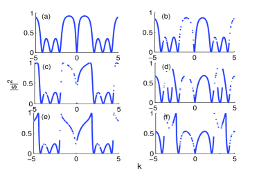
Figure 2: (color online) The transmission coefficient $|s|^{2}$ as a function of the momentum $k$ of the incident photons. (a)-(d) correspond to different nonlinear coupling constant $g=0,0.1,-0.5,0.5,-1,$ and $1,$ respectively. The other parameters chosen are $J=1,\xi=1,\omega=2,$ and $\Omega=3.$

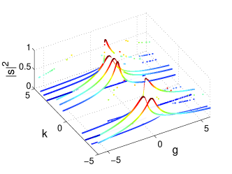
Figure 3: (color online) The transmission coefficient $|s|^{2}$ as a function of the momentum $k$ and the nonlinear coupling constant $g.$ $J=1,\xi=1,\omega=2,$ and $\Omega=3$ were chosen for this plot.

For large nonlinear coupling constants, the transmission coefficient $|s|^{2}$ is zero, as figure 3 shows. This means that the photons can not transmitted along the cavity array.

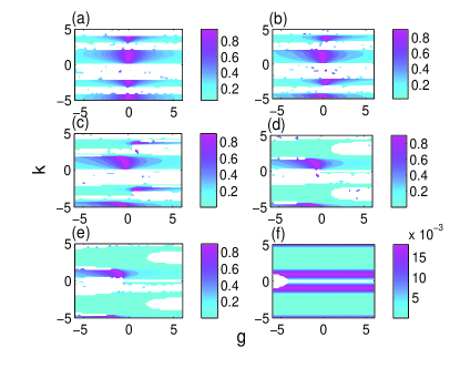
Figure 4: (color online)This contour plot shows the transmission coefficient as a function of $k$ and $g$ with different cavity-atom coupling constant $J$. (a) $J=0,$ (b) $J=0.5$, (c) $J=1,$ (d) $J=1.5,$ (e) $J=2,$ and (f) $J=5.$ The other parameters chosen are $\xi=1,\omega=2,$ and $\Omega=3$. Note that the blank regions in the figure indicate no solutions have found for $|s|^{2}$.

For $g=0$ and $J=0,$ the transmission coefficient $|s|^{2}$ is 1, however this is not the case for nonzero $g$ and $J=0,$ $|s|^{2}$ would depend on $k$. For small $g$, the nonlinear effects block the photon transport in most cases, however, for some special $k$, the nonlinearity favors the photon transmission. For large $g$, the nonlinear effect always decreases the transmission rate independent of what $k$ takes. The coupling of the atom to the photons can shift the peaks of the transmission spectrum, this is shown in figure 4.

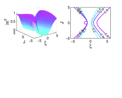
Figure 5: (color online)Transmission coefficient as a function of $J$ and $\xi$ with $k=1,g=1,\omega=2,$ and $\Omega=3.$

For fixed $k$ and $g$, the dependence of the transmission coefficient $|s|^{2}$ on $J$ and $\xi$ is shown in figure 5. Figure 4 shows that the peak of the transmission spectrum is symmetric about $g=0$ when $J=0.$ As the coupling constat $J$ increases, the peaks are shifted and lose the symmetry about $g$, i.e., the stronger the atom-field coupling, the bigger the peak shift. Two observations can be found from figure 5. (1) For a fixed $J$, the transmission coefficient $|s|^{2}$ increases with $\xi$. This can be easily understood as that large $\xi$ would increase the photon transmitting, resulting in larger $|s|^{2}.$ (2) For a fixed $\xi$, the dependence of the transmission coefficient $|s|^{2}$ on $J$ behaves different for positive and negative $\xi$. For $\xi>0$, $|s|^{2}$ increases as $|J|$ decreases, whereas for $\xi<0$, $|s|^{2}$ becomes larger with $|J|$ decreases.

IV dynamics

To gain insight of the nonlinear effect on the transport of photons along the cavity array, we numerically simulate the dynamics of the system, and present the numerical results in this section. For this purpose, we first rescall the Hamiltonian $H=H_{c}+H_{I}$ by the total number of photons in these cavities. Notice that for a very large number of photons, $M=\langle\hat{M}\rangle\gg 1$ with $\hat{M}=\sum_{i}a_{i}^{\dagger}a_{i},$ the total number of photons is (approximately) a constant of motion for the system. So, we may simulate the dynamics by using a Hamiltonian obtained by replacing $a_{i}^{\dagger},a_{i}$ with $a_{i}^{\dagger}/\sqrt{M},a_{i}/\sqrt{M},$ respectively, this leads to a set of coupled equations which have the same form as in Eq.(4), but with rescaled constants, $\omega_{r}=\omega,$ $\xi_{r}=\xi,$ $g_{r}=M\cdot g,$ $\Omega_{r}=\Omega,$ and $J_{r}=J/\sqrt{M}.$ We plot the photon number in the $-1$th (blue and dashed line) and $+1$th (red and solid line) cavities as a function of time in Fig.6 and Fig.7. The initial state of photons is all photons (total number $M=15$) in the $-1$th cavity, while the atom initially is in its excited state $|e\rangle.$ The $-1$th cavity is the first cavity left of the atom, and the $+1$th one is the first on the right, the atom occupies the $0$th cavity, as we described before. Fig.6 shows that for resonantly atom-field coupling (Fig.6-(a)), the photon in the both cavities arrive in a synchronizely changed state for a very short time. As the detuning $(\omega-\Omega)$ increases, it needs a longer time to evolve into such a state (see Fig.6-(b),(c)). We also find from Fig.6 that for resonantly atom-field coupling, it is easier for the photons to transfer through the $0$th cavity than the case of non-resonant coupling. This can be found by observing the first peak of the red-solid curve, obviously, the first peak of the red-solid line in Fig.6-(a) is higher than that in (b) and (c).

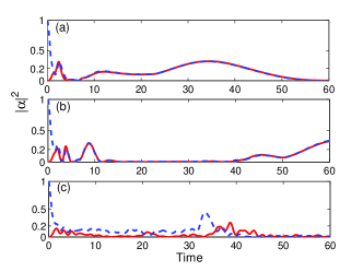
Figure 6: (color online) Photon number in $-1$th cavity (blue and dashed line) and $+1$th cavity (red and solid line) as a function of time. The parameters chosen are $\omega_{r}=2,$ $J_{r}=15,$ $M=15,$ $\xi_{r}=1,$ $g_{r}=2.$ (a) $\Omega_{r}=2,$ (b)$\Omega_{r}=3,$ and (c) $\Omega_{r}=5.$

Fig.7 shows the nonlinear effect on the dynamics of the system. Again, the nonlinearity affects the time needed for the cavity field to evolve into a synchronized state. The larger the nonlinear coupling constant $g$ is, the longer the time to arrive at such a state. Fig.7 also shows that the nonlinear effect blocks the photon transfer along the cavity array with strong nonlinearity, reminiscent of the self-trapping for Bose-Eintein condensates in a double-well potential.

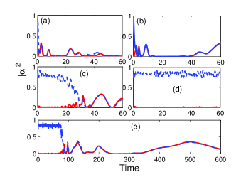
Figure 7: (color online) The same as Fig.6, but with different parameters. $\omega_{r}=2,$ $\Omega_{r}=3.$ (a) $g_{r}=0.5,$ (b) $g_{r}=2,$ (c) $g_{r}=2.9,$ (d) $g_{r}=3.$ (e) is a long time plot for (d).

V Possible Experimental observation

In this section, we propose an experimentally accessible quantum system to demonstrate our theoretical predictions for the transmission coefficient $|s|^{2}.$ Consider a system of $(2N+1)$ single-mode coupled nonlinear waveguides ( denoted as $-N,-N+1,-N+2,...,-1,0,1,...,N-1,N,$ see figure 8). The

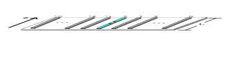
Figure 8: (color online)A schematic illustration of the setup. The relative distance between the coupled waveguides equal to each other, resulting in the same coupling constant among the neighboring waveguides. The two-level atom was put in the zeroth waveguide in the center.

waveguides are identical in shape and have a constant widthlahini08 along the propagation direction $z$. The distances between the waveguides equal to each other, as a consequence, the coupling constants between the waveguides remain unchanged along the propagation. $L$ denotes the waveguide length. We assume that only couplings between neighboring waveguides are practically nonzero in this configuration. The two-level atom is put in the zeroth waveguide. The waveguides can be designed to have a width of $3\mu m$ and length of $18mm.$ The edge-to-edge distance between waveguides is $5\mu m$, yielding a coupling constant of 2500 $m^{-1}$. The evolution of the modal amplitudes in those waveguides can be described by Eq.(4) in the intensive light limit. The nonlinear couplings $g$ stem from the Kerr nonlinear coefficient of the waveguides. These couplings are important only in the nonlinear regime and can be neglected at low light power levels. We would like to note that $\dot{A}$ in Eq.(5) should be understood as $\partial A/\partial z$ $(A=a_{j},\sigma_{+},\sigma_{-},\sigma_{z},j=0,1,2,...)$ in this coupled waveguide system. The waveguides used in this proposal can be fabricated on an $AlGaAs$ substrate, using standard photolithography techniquesmandelik05 . Indeed by this configuration in three coupled waveguides, the effect of nonlinearity on adiabatic evolution of of light was observedlahini08 . Besides, these features that result from the effect of nonlinearity can also hopefully be observed in coupled superconducting transmission line resonators.

VI conclusion

To sum up, taking nonlinear couplings of photons into account, we have studied theoretically the transmission properties of intensive light in a one-dimensional waveguide. The transmission coefficient was calculated and discussed. These results show that the nonlinear couplings sharply influence the transmission, and the atom-field couplings shift the peaks in the transmission spectrum. The dependence of the transmission coefficient on the couplings between the neighboring sites is also calculated and analyzed. Besides, we numerically simulate the dynamics of the system. The following features are found. (1) Resonant atom-field coupling favors the photon transport, the larger the detuning is, the longer the time needed to arrive at a synchronized state. (2) Nonlinearity blocks the transfer of photons among the cavity array, and postpone the time to arrive at a synchronized state. (3) Both a off-resonant atom-field coupling and a strong nonlinearity make the photon transport along the cavity array difficult with respect to the case of resonant atom-field coupling and without (or small) nonlinearity.

This work was supported by NSF of China under Grant No. 10775023.

References

- (1) D. K. Armani, T.J. Kippenberg, S.M. Spillane and K.J. Vahala, Nature 421, 925 (2003).
- (2) T. Aoki, B. Dayan, E. Wilcut, W. P. Bowen, A.S. Parkins, H. J. Kimble, T.J. Kippenberg and K.J. Vahala, Nature 443, 825 (2006).
- (3) P.E. Barclay, K. Srinivasan, O. Painter, B. Lev and H. Mabuchi, Appl. Phys. Lett. 89, 131108 (2006).
- (4) Y. Akahane, T. Asano, B. S. Song and S. Noda, Nature 425, 944 (2003).
- (5) K. Hennessy, A. Badolato, M. Winger, D. Gerace, M. Atatüre, S. Gulde, S. Fält, E.L. Hu and A. Imamoglu, Nature 445, 896 (2007).
- (6) A. Wallraff, D.I. Schuster, A. Blais, L. Frunzio, R.- S. Huang, J. Majer, S. Kumar, S.M. Girvin and R.J. Schoelkopf, Nature 431, 162 (2004).
- (7) M. Trupke, J. Goldwin, B. Darquié, G. Dutier, S. Eriksson, J. Ashmore and E. A. Hinds, Phys. Rev. Lett. 99, 063601 (2007).
- (8) Y. Colombe, T. Steinmetz, G. Dubois, F. Linke, D. Hunger and J. Reichel, Nature 450, 272 (2007).
- (9) J. T. Shen, Shanhui Fan, Phys. Rev. Lett. 95, 213001(1995); J. T. Shen, Shanhui Fan, Optics Letters 30, 2001(2005).
- (10) Lan Zhou, Z. R. Gong, Yu-xi Liu, C. P. Sun, Franco Nori, Phys. Rev. Lett 101, 100501 (2008); Lan Zhou, H. Dong, Yu-xi Liu, C. P. Sun, Franco Nori, Phys. Rev. A 78, 063827 (2008).
- (11) Y. Xu, Y. Li, R. K. Lee, and A. Yariv, Phys. Rev. E 62, 7389(2000); T. S. Tsoi and C. K. Law, Phys. Rev. A 78, 063832(2008).
- (12) K. K. Likharev, Rev. Mod. Phys 51, 101(1979).
- (13) S. V. Pereverzev, A. Loshak, S. Backhaus, J. C. Davis, and R. E. Packark, Nature (London) 388, 449(1997).
- (14) K. Sukhatme, Y. Mukharsky, T. Chui, and D. Pearson, Nauture (London) 411, 280(2001).
- (15) M. Albiez, R. Gati, J. Fölling, S. Hunsmann, M. Cristiani, and M. K. Oberthaler, Phys. Rev. Lett. 95, 010402(2005).
- (16) L. Zhou, J. Lu, and C. P. Sun, Phys. Rev. A 76, 012313 (2007).
- (17) F.M. Hu, L. Zhou, T. Shi, C. P. Sun, Phys. Rev. A 76, 013819 (2007).
- (18) M.J. Hartmann, F. G. S. L. Brandao, and M. B. Plenio, Nat. Phys. 2, 849 (2006).
- (19) A.L. Rakhmanov, A. M. Zagoskin, S. Savelev, F. Nori, Phys. Rev. B 77, 144507 (2008).
- (20) Y. Lahini, F. Pozzi, M. Sorel, R. Morandotti, D. N. Christodoulides and Y. Silberberg, arXiv:0802.1027v2.
- (21) D. Mandelik, Y. Lahini and Y. Silberberg, Phys. Rev. Lett. 95, 073902(2005).