On the Penetration of Meridional Circulation below the Solar Convection Zone II: Models with Convection Zone, the Taylor-Proudman constraint and Applications to Other Stars.

Abstract

The solar convection zone exhibits a strong level of differential rotation, whereby the rotation period of the polar regions is about 25-30% longer than the equatorial regions. The Coriolis force associated with these zonal flows perpetually “pumps” the convection zone fluid, and maintains a quasi-steady circulation, poleward near the surface. What is the influence of this meridional circulation on the underlying radiative zone, and in particular, does it provide a significant source of mixing between the two regions? In Paper I, we began to study this question by assuming a fixed meridional flow pattern in the convection zone and calculating its penetration depth into the radiative zone. We found that the amount of mixing caused depends very sensitively on the assumed flow structure near the radiative–convective interface. We continue this study here by including a simple model for the convection zone “pump”, and calculating in a self-consistent manner the meridional flows generated in the whole Sun. We find that the global circulation timescale depends in a crucial way on two factors: the overall stratification of the radiative zone as measured by the Rossby number times the square root of the Prandtl number, and, for weakly stratified systems, the presence or absence of stresses within the radiative zone capable of breaking the Taylor-Proudman constraint. We conclude by discussing the consequences of our findings for the solar interior and argue that a potentially important mechanism for mixing in Main Sequence stars has so far been neglected.

1 Introduction

Various related mechanisms are thought to contribute to the generation and maintenance of large-scale meridional flows in the solar convection zone. The effect of rotation on turbulent convection induces a relatively strong anisotropy in the Reynolds stresses (Kippenhahn 1963), in particular near the base of the convection zone where the convective turnover time is of the order of the solar rotation period. The divergence of these anisotropic stresses can directly drive large-scale meridional flows (see Rüdiger, 1989, for a discussion of this effect). It also drives large-scale zonal flows (more commonly referred to as differential rotation) which then induce meridional forcing through the biais of the Coriolis force, a mechanism referred to as “gyroscopic pumping” (McIntyre 2007). Indeed, the polar regions of the convection zone are observed to be more slowly rotating than the bulk of the Sun (Schou et al. 1998), so that the associated Coriolis force in these regions drives fluid towards the polar axis. Meanwhile, equatorial regions are rotating more rapidly than the average, and are therefore subject to a Coriolis force pushing fluid away from the polar axis. The most likely flow pattern resulting from the combination of these forces is one with an equatorial upwelling, a surface poleward flow and a deep return flow. This pattern is indeed observed near the solar surface: poleward surface and sub-surface flows with velocities up to a few tens of meters per second have been observed by measurements of photospheric line-shifts (Labonte & Howard 1982) and by time-distance helioseismology (Giles et al. 1997) respectively.

The amplitude and spatial distribution of these meridional flows deeper in the convection zone remains essentially unknown, as the sensitivity of helioseismic methods rapidly drops below the surface. As a result, the question of whether some of the pumped mass flux actually penetrates into the underlying radiative zone is still open, despite its obvious importance for mixing of chemical species (Pinsonneault, 1997; Elliott & Gough, 1999), and its presumed role in the dynamical balance of the solar interior (Gough & McIntyre 1998, McIntyre, 2007, Garaud, 2007, Garaud & Garaud, 2008) and in some models of the solar dynamo (see Charbonneau, 2005 for a review).

In Paper I (Garaud & Brummell, 2008), we began a systematic study of the penetration of meridional flows from the convection zone into the radiative zone by considering a related but easier question: assuming that the amplitude and geometry of meridional flows in the convection zone are both known, what is their influence on the underlying radiative zone? This simpler question enabled us to study the dynamics of the radiative zone only by assuming a flow profile at the radiative–convective interface (instead of having to include the more complex convection zone in the calculation). The overwhelming conclusion of that first study was that the degree to which flows penetrate into the stratified interior (in the model) is very sensitive to the interfacial conditions selected. Hence, great care must be taken when using a “radiative-zone-only” model to make definite predictions about interior flow amplitudes. In addition, that approach makes the implicit assumption that the dynamics of the radiative zone do not in return influence those of the convection zone, but the only way to verify this is to construct a model which includes both regions. This was the original purpose of the present study; as we shall see, the combined radiative–convective model we construct here provides insight into a much broader class of problems.

We therefore propose a simplified model of the Sun which includes both a “convective” region and a “radiative” region, where the convective region is forced in such a way as to promote gyroscopic pumping of meridional flows. We calculate the flow solution everywhere and characterize how it scales in terms of governing parameters (e.g. stellar rotation rate, stratification, diffusivities, etc..), focusing in particular on the flows which are entering the radiative zone. We begin with a simple Boussinesq Cartesian model (Section 2), first in the unstratified limit (Section 2.3) and then in the more realistic case of a radiative–convective stratification (Section 2.4). Although the Cartesian results essentially illustrate most of the relevant physical phenomena, we confirm our analysis with numerical solutions of the full set of equations in a spherical geometry in Section 3. We then use this information in Section 4 to discuss the effects of mixing by meridional flows both in the Sun and in other Main Sequence stars.

2 A Cartesian model

2.1 Model setup

As in Paper I, we first study the problem in a Cartesian geometry. Since our primary aim is to understand the behavior of the meridional flows generated (e.g. scaling of the solutions) in terms of the governing parameters, this approach is sufficient and vastly simplifies the required algebra. In Section 3, we turn to numerical simulations to study the problem in a spherical geometry.

In this Cartesian model section, distances are normalized to the solar radius $R_{\odot}$, and velocities to $R_{\odot}\Omega_{\odot}$ where $\Omega_{\odot}$ is the mean solar angular velocity (the exact value is not particularly relevant here). The coordinate system is $(x,y,z)$, where $x$ should be thought of as the azimuthal coordinate $\phi$, with $x\in[0,2\pi]$; $y$ represents minus the co-latitude and spans the interval $y\in[0,\pi]$ (the poles are at $y=0$ and $y=\pi$ while the equator is at $y=\pi/2$). Finally the $z$-direction is the radial direction with $z\in[0,1]$, and represents the direction of (minus) gravity so that $z=0$ is the interior, and $z=1$ is the surface.

In this framework, the system rotates with mean angular velocity $\mbox{\boldmath$\Omega$}=(0,0,1)$, thereby implicitly assuming that the rotation axis is everywhere aligned with gravity. This assumption induces another “geometric” error in the velocity estimates for the meridional flows, comparable with the error made in reducing the problem to a Cartesian analysis; it does not influence the predicted scalings (except in small equatorial regions which we ignore here).

We divide the domain in two regions, by introducing the dimensionless constant $h$ to represent the radiative–convective interface. Thus $z\in[0,h]$ represents the “radiative zone” while $z\in[h,1]$ represents the “convection zone”. From here on, $h=0.7$. Figure 1 illustrates the geometry of the Cartesian system.

Figure 1: Cartesian model geometry and intended correspondence with the spherical case. The shaded area marks the convective region, where forcing is applied. The $y=0$ and $y=\pi/2$ lines mark the “poles” and the “equator”. The system is assumed to be periodic with period $\pi$ in the $y-$direction.

2.2 Model equations

For this simple Cartesian approach, we work with the Boussinesq approximation (this assumption is dropped in the spherical model but doesn’t affect the predicted scalings). The background state is assumed to be stratified, steady, and in hydrostatic equilibrium. The background density and temperature profiles are denoted by $\bar{T}(z)$ and $\bar{\rho}(z)$ respectively. Density and temperature perturbations to this background state ($\rho$ and $T$) are then assumed to be linearly related: $\rho=-\alpha_{T}(z)T$, where $\alpha_{T}(z)$ is the coefficient of thermal expansion. For simplicity, we will assume that the background temperature gradient $\bar{T}_{z}$ is constant throughout the domain $z\in[0,1]$, and treat the convection zone as a region where $\alpha_{T}\rightarrow 0$ while the radiative zone has $\alpha_{T}\neq 0$ (see below). The alternative option of using a constant $\alpha_{T}$ and a varying $\bar{T}_{z}$ yields qualitatively equivalent scalings for the meridional flows (a statement which is verified in Section 3) although the algebra is trickier.

The set of equations governing the system in this approximation are the momentum, mass and thermal energy conservation equations respectively:

$$\frac{\partial{\bf u}}{\partial t}+{\bf u}\cdot{\mathbf{\nabla}}{\bf u}+2{\bf e}_{z}\times{\bf u}=-\nabla p+{\rm Ro}^{2}(z)T{\bf e}_{z}+{\rm E}_{\nu}{\mathbf{\nabla}}^{2}{\bf u}\mbox{ , }$$

$${\mathbf{\nabla}}\cdot{\bf u}=0\mbox{ , }$$

$$\frac{\partial T}{\partial t}+{\bf u}\cdot{\mathbf{\nabla}}T+{\bf u}\cdot{\bf e}_{z}=\frac{{\rm E}_{\nu}}{\rm Pr}{\mathbf{\nabla}}^{2}T\mbox{ , }$$ (1)

where ${\bf u}=(u,v,z)$ is the velocity field. In these equations, temperature perturbations have been normalized to the background temperature difference across the box $R_{\odot}\bar{T}_{z}$. The governing non-dimensional parameters are:

$${\rm Ro}(z)=N(z)/\Omega_{\odot}\mbox{ the Rossby number }\mbox{ , }$$

$${\rm E}_{\nu}=\frac{\nu}{R_{\odot}^{2}\Omega_{\odot}}\mbox{ the Ekman number }\mbox{ , }$$

$${\rm Pr}=\frac{\nu}{\kappa_{T}}\mbox{ the Prandtl number }\mbox{ , }$$ (2)

where the dimensional quantity $N^{2}(z)=\alpha_{T}(z)\bar{T}_{z}g$ is the square of the Brunt-Väisälä frequency ($g$ is the magnitude of gravity and is assumed to be constant). The microscopic diffusion coefficients $\nu$ (the viscosity) and $\kappa_{T}$ (the thermal conductivity) are both assumed to be constant. In the Sun, near the radiative–convective interface, ${\rm E}_{\nu}\simeq 2\times 10^{-15}$ and Pr $\simeq 2\times 10^{-6}$ (Gough, 2007).

As mentioned earlier, the transition between the model radiative zone and convection zone is measured by the behavior of $\alpha_{T}(z)$, which goes from 0 for $z>h$ to a finite value for $z<h$. This can be modeled in a non-dimensional way through the Rossby number, which we assume is of the form:

$${\rm Ro}(z)=\frac{{\rm Ro}_{\rm rz}}{2}\left[1+\tanh\left(\frac{h-z}{\Delta}\right)\right]\mbox{ , }$$ (3)

where ${\rm Ro}_{\rm rz}$ is constant. The lengthscale $\Delta$ may be thought of as the thickness of the “overshoot” region near the base of the convection zone, but in practise is mostly used to ensure continuity and smoothness of the background state through the tanh function.

In what follows, we further restrict our study to an “axially” symmetric $(\partial/\partial x=0)$, steady-state $(\partial/\partial t=0)$ problem. Within the radiative zone, the nonlinear terms ${\bf u}\cdot{\mathbf{\nabla}}{\bf u}$ and ${\bf u}\cdot{\mathbf{\nabla}}T$ are assumed to be negligible. Within the convection zone on the other hand, anisotropic turbulent stresses are thought to drive the observed differential rotation. We model this effect in the simplest possible way, replacing the divergence of the stresses by a linear relaxation towards the observed convection zone profile:

$${\bf u}\cdot{\mathbf{\nabla}}{\bf u}\rightarrow{\bf F}_{\rm turb}=\frac{{\bf u}-{\bf u}_{\rm cz}}{\tau}\mbox{ , }$$ (4)

where ${\bf u}_{\rm cz}=u_{\rm cz}(y,z){\bf e}_{x}$ and the function $u_{\rm cz}(y,z)$ models the observed azimuthal velocity profile in the solar convection zone. This is analogous to the prescription used by Spiegel & Bretherton (1968) in their study of the effect of a convection zone on solar spin-down, although in their model the convection zone was not differentially rotating. The dimensionless relaxation timescale $\tau$ can be thought of, for example, as being of the same order of magnitude as the convective turnover time divided by the rotation period. It is modeled as:

$$\tau^{-1}(z)=\frac{\Lambda}{2}\left[1+\tanh\left(\frac{z-h}{\Delta}\right)\right]\mbox{ . }$$ (5)

Note that in the real solar convection zone, $\tau$ varies by orders of magnitudes between the surface ($\tau\sim 10^{-3}$) and the bottom of the convection zone ($\tau\sim 1$). Here, we assume that $\Lambda$ is constant for simplicity.

We adopt the following profile for $u_{\rm cz}(y,z)$:

$$u_{\rm cz}(y,z)=\frac{U_{0}(z)}{2}\left[1+\tanh\left(\frac{z-h}{\Delta}\right)\right]e^{iky}=\hat{u}_{\rm cz}(z)e^{iky}\mbox{ , }$$

$$U_{0}(z)=U_{0}(h)+S(z-h)\mbox{ , }$$ (6)

where $k=2$ to match the equatorial symmetry of the observed solar rotation profile. The tanh function once again is merely added to guarantee continuity of the forcing across the overshoot layer. The function $U_{0}(z)$ describes the imposed “vertical shear”, and is for simplicity taken to be a linear function of $z$. If $U_{0}(h)=0$, the forcing effectively vanishes at the base of the convection zone. If $U_{0}(h)\neq 0$ on the other hand, a strong azimuthal shear is forced at the interface. The observed solar rotation profile appears to be consistent with $U_{0}(h)$ and $S$ both being non-zero (and of the order of 0.1, although since we are studying a linear problem, the amplitude of the forcing is somewhat irrelevant). Note that if $S=0$ the forcing velocity ${\bf u}_{\rm cz}$ has zero vorticity.

Finally, the observed asphericity in the temperature profile is negligible in the solar convection zone; this is attributed to the fact that the turbulent convection very efficiently mixes heat both vertically and horizontally. We model this effect as:

$${\bf u}\cdot{\mathbf{\nabla}}T\rightarrow-D(z){\mathbf{\nabla}}^{2}T\mbox{ , }$$ (7)

where the turbulent heat diffusion coefficient is modeled as

$$D(z)=\frac{D_{0}}{2}\left[1+\tanh\left(\frac{z-h}{\Delta}\right)\right]\mbox{ , }$$ (8)

and thus vanishes beneath the overshoot layer. We will assume that the diffusion timescale $1/D_{0}$ (in non-dimensional units) is much smaller than any other typical timescale in the system ($D_{0}\gg 1$).

Projecting the remaining equations into the Cartesian coordinate system, and seeking solutions in the form $q(y,z)=\hat{q}(z)e^{iky}$ for each of the unknown quantities yields

$$-2\hat{v}={\rm E}_{\nu}\left(\frac{{\rm d}^{2}\hat{u}}{{\rm d}z^{2}}-k^{2}\hat{u}\right)-\frac{\hat{u}-\hat{u}_{\rm cz}}{\tau}\mbox{ , }$$

$$2\hat{u}=-ik\hat{p}+{\rm E}_{\nu}\left(\frac{{\rm d}^{2}\hat{v}}{{\rm d}z^{2}}-k^{2}\hat{v}\right)-\frac{\hat{v}}{\tau}\mbox{ , }$$

$$0=-\frac{{\rm d}\hat{p}}{{\rm d}z}+{\rm Ro}^{2}(z)\hat{T}+{\rm E}_{\nu}\left(\frac{{\rm d}^{2}\hat{w}}{{\rm d}z^{2}}-k^{2}\hat{w}\right)-\frac{\hat{w}}{\tau}\mbox{ , }$$

$$ik\hat{v}+\frac{{\rm d}\hat{w}}{{\rm d}z}=0\mbox{ , }$$

$$\hat{w}=\left(\frac{{\rm E}_{\nu}}{\rm Pr}+D(z)\right)\left(\frac{{\rm d}^{2}\hat{T}}{{\rm d}z^{2}}-k^{2}\hat{T}\right)\mbox{ , }$$ (9)

Note that as required, the imposed forcing term drags the fluid in the azimuthal direction: for $\tau\rightarrow 0$, $\hat{u}\rightarrow\hat{u}_{\rm cz}$ in the convection zone. The meridional flows $\hat{v}$ and $\hat{w}$ on the other hand are generated by the $y-$component of the Coriolis force and by mass conservation respectively (the essence of gyroscopic pumping, see McIntyre 2007).

We now proceed to solve these equations to gain a better understanding of the meridional flows and their degree of penetration into the radiative zone below. We use a dual approach, solving these equations first analytically under various limits, and then exactly using a simple Newton-Raphson-Kantorovich (NRK) two-point boundary value algorithm. The analytical approximations yield predictions for the relevant scalings of the solutions in terms of the governing parameters (an in particular, the Ekman number and the Rossby number) which are then confirmed by the exact numerical solutions.

2.3 The unstratified case

Although this limit is not a priori relevant to the physics of the solar interior, we begin by studying the case of an unstratified region, setting ${\rm Ro}_{\rm rz}=0$ (in this case, the thermal energy equation can be discarded). This simpler problem, as we shall demonstrate, contains the essence of the problem.

In order to find analytical approximations to the solutions, we solve the governing equations separately in the convective zone and in the radiative zone. At this point, it may be worth pointing out that in the unstratified case, the nomenclatures “convective” and “radiative” merely refer to regions which respectively are and are not subject to the additional forcing.

We assume that the transition region is very thin. In this case, $\tau^{-1}=\Lambda$ for $z>h$ while $\tau^{-1}=0$ for $z<h$. Similarly, $\hat{u}_{\rm cz}(z)=U_{0}(h)+S(z-h)$ in the convection zone while $\hat{u}_{\rm cz}(z)=0$ in the radiative zone. Once obtained, the solutions are patched at the radiative–convective interface.

2.3.1 Solution in the convection zone

In the convection zone, the equations reduce to

$$-2\hat{v}=-\Lambda(\hat{u}-\hat{u}_{\rm cz})\mbox{ , }$$

$$2\hat{u}=-ik\hat{p}-\Lambda\hat{v}\mbox{ , }$$

$$0=-\frac{{\rm d}\hat{p}}{{\rm d}z}-\Lambda\hat{w}\mbox{ , }$$

$$ik\hat{v}+\frac{{\rm d}\hat{w}}{{\rm d}z}=0\mbox{ , }$$ (10)

where we have neglected the viscous dissipation terms in favor of the forcing terms since $E_{\nu}\ll\Lambda$ for all reasonable solar parameters. Combining them yields

$$\frac{{\rm d}^{2}\hat{w}}{{\rm d}z^{2}}=\frac{k^{2}\Lambda^{2}}{4+\Lambda^{2}}\hat{w}+2ik\frac{\Lambda}{4+\Lambda^{2}}\frac{{\rm d}\hat{u}_{\rm cz}}{{\rm d}z}\mbox{ . }$$ (11)

This second-order ordinary differential equation for $\hat{w}(z)$ suggests the introduction of a new lengthscale

$$\delta=\frac{\sqrt{4+\Lambda^{2}}}{k\Lambda}\mbox{ , }$$ (12)

so that the general solution to (10) is

$$\hat{w}(z)=Ae^{z/\delta}+Be^{-z/\delta}-\frac{2iS}{k\Lambda}\mbox{ , }$$

$$\hat{v}(z)=-\frac{1}{ik\delta}\left[Ae^{z/\delta}-Be^{-z/\delta}\right]\mbox{ , }$$

$$\hat{u}(z)=\hat{u}_{\rm cz}(z)-\frac{2}{ik\Lambda\delta}\left[Ae^{z/\delta}-Be^{-z/\delta}\right]\mbox{ , }$$

$$\hat{p}(z)=-\frac{2}{ik}\hat{u}_{\rm cz}(z)-\delta\Lambda\left[Ae^{z/\delta}-Be^{-z/\delta}\right]\mbox{ . }$$ (13)

The constants $A$ and $B$ are integration constants which must be determined by applying boundary conditions (at $z=1$) and matching conditions (at $z=h$). Note from the $\hat{u}$-equation that the actual rotation profile approaches the imposed (observed) profile $\hat{u}_{\rm cz}$ provided $A$ and $B$ tend to 0, or when $\Lambda\gg 2$ (in which case $\delta\rightarrow 1/k$).

2.3.2 Solution in the radiative zone with stress-free lower boundary, and matching

In the radiative region, the equations reduce to

$$-2\hat{v}={\rm E}_{\nu}\left(\frac{{\rm d}^{2}\hat{u}}{{\rm d}z^{2}}-k^{2}\hat{u}\right)\mbox{ , }$$

$$2\hat{u}=-ik\hat{p}\mbox{ , }$$

$$\frac{{\rm d}\hat{p}}{{\rm d}z}=0\mbox{ , }$$

$$ik\hat{v}+\frac{{\rm d}\hat{w}}{{\rm d}z}=0\mbox{ , }$$ (14)

if we neglect viscous stresses in both $y$ and $z$ components of the momentum equation. Note that viscous stresses in the $x-$equation cannot be dropped since they are the only force balancing the Coriolis force. These equations are easily solved:

$$\hat{p}(z)=p_{\rm rz}\mbox{ , }$$

$$\hat{u}(z)=-\frac{ik}{2}p_{\rm rz}\mbox{ , }$$

$$\hat{v}(z)=-\frac{iE_{\nu}k^{3}}{4}p_{\rm rz}\mbox{ , }$$

$$\hat{w}(z)=w_{\rm rz}-\frac{E_{\nu}k^{4}}{4}p_{\rm rz}z\mbox{ , }$$ (15)

where $p_{\rm rz}$ and $w_{\rm rz}$ are two additional integration constants. Here, we recover the standard Taylor-Proudman constraint where in the absence diffusion or any other stresses, the velocity must be constant along the rotation axis (here, ${\bf e}_{z}$); in the limit ${\rm E}_{\nu}\rightarrow 0$, $\hat{u}(z)$ and $\hat{w}(z)$ become independent of $z$, while $\hat{v}(z)\rightarrow 0$.

We are now able to match the solution in the radiative zone to that of the convection zone. The two constants $p_{\rm rz}$ and $w_{\rm rz}$ form, together with $A$ and $B$, a set of 4 unknown constants which are determined by application of boundary and matching conditions. Since we have neglected viscous effects in the convection zone, we cannot require any boundary or matching condition on the horizontal fluid motions. On the other hand, we are allowed to impose impermeability $\hat{w}=0$ at the surface ($z=1$) and at the bottom ($z=0$). Moreover, we request the continuity of the radial (vertical) velocity and of the pressure at the interface ($z=h$). Applying these conditions yields the set of equations

$$w_{\rm rz}=0\mbox{ , }$$

$$Ae^{h/\delta}+Be^{-h/\delta}-\frac{2iS}{k\Lambda}=w_{\rm rz}-\frac{{\rm E}_{\nu}k^{4}}{4}p_{\rm rz}h\mbox{ , }$$

$$-\frac{2}{ik}U_{0}(h)-\delta\Lambda\left[Ae^{h/\delta}-Be^{-h/\delta}\right]=p_{\rm rz}\mbox{ , }$$

$$Ae^{1/\delta}+Be^{-1/\delta}-\frac{2iS}{k\Lambda}=0\mbox{ , }$$ (16)

which have the following solution for $A$ and $B$:

$$A=\frac{\frac{{\rm E}_{\nu}hk^{3}}{2i}U_{0}(h)+\frac{2iS}{k\Lambda}\left[1-e^{(1-h)/\delta}\left[1+\frac{E_{\nu}k^{4}}{4}h\delta\Lambda\right]\right]}{e^{h/\delta}\left[1-\frac{E_{\nu}k^{4}}{4}h\delta\Lambda\right]-e^{(2-h)/\delta}\left[1+\frac{E_{\nu}k^{4}}{4}h\delta\Lambda\right]}\mbox{ , }$$

$$B=\frac{2iS}{k\Lambda}e^{1/\delta}-Ae^{2/\delta}\mbox{ . }$$ (17)

These can be substituted back into (2.3.1) to obtain the meridional flow velocities in the convection zone. While the exact form of $A$ and $B$ are not particularly informative, we note that in the limit $S=0$ (i.e. the forcing velocity has no azimuthal vorticity), both $A$ and $B$ scale as ${\rm E}_{\nu}$. This implies that the amplitude of meridional flows everywhere in the solar interior scales like ${\rm E}_{\nu}$ (even in the convection zone). The physical interpretation of this somewhat surprising limit is discussed in Section 2.3.4, but turns out to be of academic interest only (Section 2.3.5).

When $S\neq 0$ then $A$ and $B$ are of order $S/k\Lambda$ in the convection zone regardless of the Ekman number, and respectively tend to

$$A=\frac{2iS}{k\Lambda}\frac{1-e^{(1-h)/\delta}}{e^{h/\delta}-e^{(2-h)/\delta}}+O({\rm E}_{\nu})\mbox{ , }$$

$$B=\frac{2iS}{k\Lambda}\frac{1-e^{(h-1)/\delta}}{e^{-h/\delta}-e^{(h-2)/\delta}}+O({\rm E}_{\nu})\mbox{ , }$$ (18)

as ${\rm E}_{\nu}\rightarrow 0$. This implies that $\hat{w}$ is of order $S/k\Lambda$ in the convection zone. Since significant flows are locally generated, one may reasonably expect a fraction of the forced mass flux to penetrate into the lower region, especially in this unstratified case.

Using (2.3.2) in (2.3.2), solving for $p_{\rm rz}$, then plugging $p_{\rm rz}$ into (2.3.2), we find that the general expression for $\hat{w}(z)$ in the radiative zone $z\in[0,h]$ is

$$\hat{w}(z)=-\frac{iE_{\nu}k^{3}}{2}\left(U_{0}(h)+\frac{\cosh((1-h)/\delta)-1}{\sinh((1-h)/\delta)}\delta S\right)z\mbox{ . }$$ (19)

This implies that only a tiny fraction of the large mass flux circulating in the convection zone actually enters the radiative zone. Instead, the system adjusts itself in such a way as to ensure that most of the meridional flows return above the base of the convection zone.

We now compare this a priori counter-intuitive analytical result with exact numerical solutions of the governing equations. The numerical solutions were obtained by solving (9) for Ro${}_{\rm rz}=0$ (unstratified case), and are uniformly calculated in the whole domain (i.e. there is nothing special about the interfacial point $z=h$). The boundary conditions used are impermeable boundary conditions at the top and bottom of the domain for $\hat{w}$, and stress-free boundary conditions for $\hat{u}$ and $\hat{v}$.

In Figure 2 we compare numerical and analytical solutions for $\hat{w}(z)$, in a case where the forcing function parameters are $\Delta=10^{-4}$, $\Lambda=10$, $U_{0}(h)=0$ and $S=1$, for four values of the Ekman number. The analytical solution is described by equations (2.3.1) and (2.3.2) (for the convection zone) and (2.3.2) (for the radiative zone). As ${\rm E}_{\nu}\rightarrow 0$ the numerical solution approaches the analytically derived one, confirming in particular that $\hat{w}(z)\propto z{\rm E}_{\nu}$ in the radiative zone. The convection zone solution is also well-approximated in this case by the analytical formula.

Figure 2: Numerical (solid) and analytical (dashed) solutions for $|\hat{w}(z)|$, in the case of a stress-free bottom boundary. From the uppermost to lowermost curves, $E_{\nu}=10^{-3}$, $10^{-4}$, $10^{-5}$ and $10^{-6}$ respectively, confirming the analytical scaling that $\hat{w}(z)\propto{\rm E}_{\nu}z$ in the radiative zone while $\hat{w}(z)$ becomes independent of ${\rm E}_{\nu}$ in the convection zone. These solutions were obtained with forcing defined by the parameters $\Delta=10^{-4}$, $\Lambda=10$, $U_{0}(z)=S(z-h)$ and $S=1$.

A full 2D visualization of the flow for ${\rm E}_{\nu}=10^{-4}$ but otherwise the same governing parameters is shown in Figure  3. This figure illustrates more clearly the fact that the meridional flows are negligible below the interface, and mostly return within the convection zone. Note that given our choice of the forcing function $u_{\rm cz}(y,z)\propto\cos(2y)$, the induced Coriolis force does not vanish at $y=0$ or $y=\pi$ (the “poles”). This explains why the meridional flows apparently cross the polar axis in this simple model. This is merely a geometric effect: in a true spherical geometry the forcing azimuthal velocity $u_{\rm cz}(r,\theta)$ would be null at the poles, and meridional flows cannot cross the polar axis. More realistic calculations in spherical geometry are discussed in Section 3.

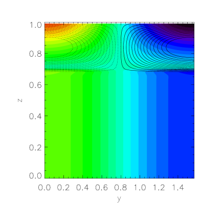
Figure 3: 2D visualization of the flow for $E_{\nu}=10^{-4}$, in the case of a stress-free bottom boundary. Shown as solid and dotted line respectively are linearly spaced streamlines of counter-clockwise and clockwise meridional flows. As predicted, the flows appear to return entirely within the convection zone and carry a negligible mass flux into the radiative zone. Meanwhile the azimuthal velocity ($\hat{u}$) as displayed in the filled contours is constant along the rotation axis ($z-$axis) below the interface ($z=h=0.7$), but is strongly sheared at the interface. This solution was obtained with forcing defined by the parameters $\Delta=10^{-4}$, $\Lambda=10$, $U_{0}(z)=S(z-h)$ and $S=1$, as in Figure 2.

Finally, it is interesting to note that the analytical solution for the azimuthal velocity $\hat{u}(z)$ exhibits a “discontinuity” across the base of the convection zone, which tends to

$$\hat{u}(h^{+})-\hat{u}(h^{-})=\left(\frac{2}{ik\delta\Lambda}+\frac{ik\delta\Lambda}{2}\right)\left(Ae^{h/\delta}-Be^{-h/\delta}\right)$$ (20)

as ${\rm E}_{\nu}\rightarrow 0$. The numerical solutions of course are continuous, but the continuity is only assured by the viscosity in the system (in the $y-$ direction) and the fact that the overshoot layer depth is finite. This is shown in Figure 4, together with a comparison of the numerical solutions with the analytical solution, again confirming the analytical approximation derived.

This highlights another and equally a priori counter-intuitive property of the system: the value of $u_{\rm rz}$ in the radiative zone is markedly different from the imposed $\hat{u}_{\rm cz}(h)=U_{0}(h)$ at the interface:

$$u_{\rm rz}=U_{0}(h)+\frac{ik\delta\Lambda}{2}\left(Ae^{h/\delta}-Be^{-h/\delta}\right)\mbox{ .}$$ (21)

Hence, even if the imposed differential rotation is exactly 0 at the radiative–convective interface (as it is the case in the simulation presented in Figure 4 since $U_{0}(z)=S(z-h)$), a large-scale latitudinal shear measured by $u_{\rm rz}$ may be present in the radiative zone, as illustrated in Figure 3. This shows that the propagation of the azimuthal shear into the radiative zone is non-local (i.e. does not rely on the presence of shear at the interface), and is instead communicated by the long-range pressure gradient.

Figure 4: Numerical (solid) and analytical (dashed) solutions for $\hat{u}(z)$, in the case of a stress-free bottom boundary. From the lowermost to uppermost curves, $E_{\nu}=10^{-3}$, $10^{-4}$, $10^{-5}$ and $10^{-6}$ respectively, confirming that $\hat{u}(z)$ tends to a constant in the radiative zone, while sustaining a finite discontinuity at the radiative-convective interface ($z=h=0.7$). These solutions were obtained with forcing defined by the parameters $\Delta=10^{-4}$, $\Lambda=10$, $U_{0}(z)=S(z-h)$ and $S=1$, as in Figure 2.

2.3.3 Solution in the case of no-slip bottom boundary

The stress-free bottom boundary conditions studied in the previous Section are at first glance the closest to what one may expect in the real Sun, where the “bottom” boundary merely represents the origin of the spherical coordinate system. However, let us now explore for completeness (and for further reasons that will be clarified in the next Section) the case of no-slip bottom boundary conditions.

When the lower boundary is a no-slip boundary, the nature of the solution in the whole domain changes. This change is induced by the presence of an Ekman boundary layer, which forms near $z=0$. Just above the boundary layer, in the bulk of the radiative zone, the solution described in 2.3.2 remains valid. However, matching the bulk solution with the boundary conditions can no longer be done directly; one must first solve for the boundary layer dynamics to match the bulk solution with the boundary conditions across the boundary layer. This is a standard procedure (summarized in Appendix A for completeness), and leads to the well-known “Ekman jump” relationship between the jump in $\hat{w}(z)$ and the jump in $\hat{u}(z)$ across the boundary layer:

$$\hat{u}_{\rm bulk}-\hat{u}(0)=\frac{2i}{k}E_{\nu}^{-1/2}(\hat{w}_{\rm bulk}-\hat{w}(0))\mbox{ . }$$ (22)

By impermeability, $\hat{w}(0)=0$. Moreover, by assuming that the total angular momentum of the lower boundary is the same as that of the convection zone, we require that $\hat{u}(0)=0$. Meanwhile, $\hat{u}_{\rm bulk}=u_{\rm rz}$ and $\hat{w}_{\rm bulk}=w_{\rm rz}$ in the notation of equation (2.3.2). So finally, for no-slip boundary conditions, we simply replace the impermeability condition ($w_{\rm rz}=0$) in (2.3.2) by

$$u_{\rm rz}=\frac{2i}{k}E_{\nu}^{-1/2}w_{\rm rz}\mbox{ , }$$ (23)

and solve for the unknown constants $A$, $B$, $w_{\rm rz}$ and $p_{\rm rz}$ as before.

The exact expressions for the resulting integration constants $A$ and $B$ are now slightly different from those given in (2.3.2), but are without particular interest. However, it can be shown that they have the same limit as in the stress-free case as ${\rm E}_{\nu}\rightarrow 0$ (with $S\neq 0$). This implies that the meridional flows driven within the convection zone, in the limit ${\rm E}_{\nu}\rightarrow 0$, and with $S\neq 0$, are independent of the boundary condition selected at the bottom of the radiative zone. However, we now have the following expression for $\hat{w}(z)$ in the bulk of the radiative zone:

$$\hat{w}(z) = -\left(\frac{k^{2}}{4}E_{\nu}^{1/2}+\frac{E_{\nu}k^{4}}{4}z\right)p_{\rm rz}\mbox{ , }$$ (24)

$$= -\frac{ik}{2}E_{\nu}^{1/2}\left(U_{0}(h)+\frac{\cosh((1-h)/\delta)-1}{\sinh((1-h)/\delta)}\delta S\right)+O({\rm E}_{\nu})z\mbox{ , }$$

which has one fundamental consequence: the amplitude of the flows allowed to penetrate into the radiative zone is now of order $E_{\nu}^{1/2}$ instead of being $O({\rm E}_{\nu})$. This particular statement is actually true even if $S=0$, although in that case both convection zone and radiative zone flows scale with $E_{\nu}^{1/2}$.

Figure 5 shows a comparison between the approximate analytical formula and the numerical solution for the same simulations as in Figure 2, but now using no-slip bottom boundary conditions. For ease of comparison, the results from the stress-free numerical simulations (for exactly the same parameters) have also been drawn, highlighting the much larger amplitude of the meridional flows down-welling into the radiative zone in the no-slip case, and their scaling with $E_{\nu}^{1/2}$. Figure 6 shows an equivalent 2D rendition of the solution, and illustrates the presence of large-scale mixing in the bulk of the radiative zone when the bottom-boundary is no-slip.

Figure 5: Numerical (solid) and analytical (dashed) solutions for $|\hat{w}(z)|$, in the case of a no-slip bottom boundary. From the uppermost to lowermost curves (as seen in the radiative zone), $E_{\nu}=10^{-3}$, $10^{-4}$, $10^{-5}$ and $10^{-6}$ respectively, confirming the analytical scaling that $\hat{w}(z)\propto{\rm E}_{\nu}^{1/2}$ in the radiative zone while $\hat{w}(z)$ becomes independent of ${\rm E}_{\nu}$ in the convection zone. These solutions were obtained with forcing defined by the parameters $\Delta=10^{-4}$, $\Lambda=10$, $U_{0}(z)=S(z-h)$ and $S=1$, as in Figure 2. For comparison, the previous simulations with stress-free bottom boundary, for the same parameters, are shown as dotted lines.

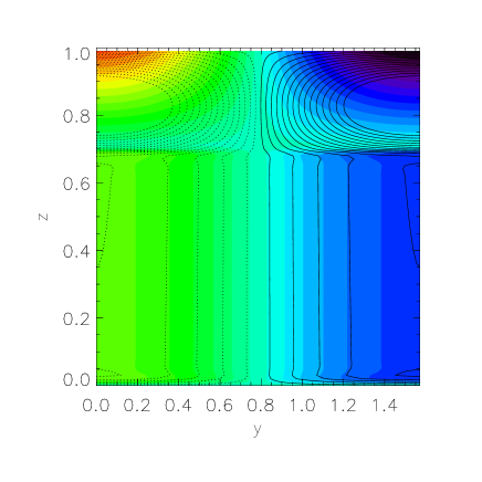
Figure 6: The same as for Figure 3 but for no-slip boundary conditions. The Ekman layer near the lower boundary is clearly visible. For ease of comparison, the same streamlines are shown in the two plots. The two figures illustrates how the nature of the lower boundary condition influences the mass flux through the radiative zone.

2.3.4 Physical interpretation

The various sets of solutions derived above can be physically understood in the following way. Let us first discuss the solution in the convection zone. In the limit where $u_{\rm cz}(y,z)$ is independent of $z$ (equivalently, $S=0$), the azimuthal ($x-$) component of the vorticity of the forcing is zero. In that case there is no injection of $x-$vorticity into the system aside from that induced in the viscous boundary layers, and the amplitude of the meridional flows generated in the convection zone scales with ${\rm E}_{\nu}$. This limit is somewhat academic in the case of the Sun, however given the observed rotation profile (see also Section 2.3.5). When $S\neq 0$, the amplitude of the induced meridional flows in the convection zone scales linearly with $S$ and is independent of viscosity.

In the radiative zone, the Taylor-Proudman constraint enforces invariance of the flow velocities along the rotation axis, except in regions where other forces balance the Coriolis force. In the non-magnetic, unstratified situation discussed in the two previous sections, the only agent capable of breaking the Taylor-Proudman constraint are viscous stresses, which are only significant in two thin boundary layers: one right below the convection zone and the other one near the bottom boundary. These two layers are the only regions where flows down-welling into the radiative zone are allowed to return to the convection zone. The question then remains of what fraction of the mass flux entering the radiative zone returns within the upper Ekman layer, and what fraction returns within the lower Ekman layer. The latter, of course, permits large-scale mixing within the radiative zone.

In the first case studied, the bottom boundary was chosen to be stress-free. This naturally suppresses the lower viscous boundary layer so that the only place where flows are allowed to return is at the radiative-convective interface. As a result, only a tiny fraction of the mass flux penetrates below $z=h$, and the turnover time of the remaining flows within the radiative zone is limited to a viscous timescale of the order of $1/{\rm E}_{\nu}\Omega_{\odot}$.

Following this reasoning, we expect and indeed find quite a different behavior when the bottom boundary is no-slip. In that case viscous stresses within the lower boundary layer break the Taylor-Proudman constraint and allow a non-zero mass flux (of order ${\rm E}_{\nu}^{1/2}$) to return near $z=0$. This flow then mixes the entire radiative zone as well, with an overall turnover time of order of $1/{\rm E}_{\nu}^{1/2}\Omega_{\odot}$ (in dimensional units).

To summarize, in this unstratified steady-state situation, the amount of mixing induced within the radiative zone by convective zone flows depends (of course) on the amplitude of the convection zone forcing, but also on the existence of a mechanism to break the Taylor-Proudman constraint somewhere within the radiative zone. That mechanism is needed in order to allow down-welling flows to return to the convection zone. But more crucially, this phenomenon implies that the dynamics of the lower boundary layer entirely control the mass flux through the system.

Here, we studied the case of viscous stresses only. One can rightfully argue that there are no expected “solid” boundaries in a stellar interior and that the overall behavior of the system should be closer to the one discussed in the stress-free case than the no-slip case. However, we chose here to study viscous stresses simply because they are the easiest available example. In real stars viscous stresses are likely to be negligible compared with a variety of other possible stresses: turbulent stresses at the interface with another convection zone, magnetic forces, etc. Nevertheless, these stresses will play a similar role in allowing flows to mix the radiative zone if they become comparable in amplitude with the Coriolis force, and help break the Taylor-Proudman constraint. This issue is discussed in more detail in Section 4.

2.3.5 The thickness of the overshoot layer

Before moving on to the more realistic stratified case, note that this unstratified system holds one final subtlety. In all simulations presented earlier, the overshoot layer depth was selected to be very small – and in particular, smaller than the Ekman layer thickness. In that case, the transition in the forcing at the base of the convection zone is indeed close to being a discontinuity, and the analytical solutions presented in Sections 2.3.1 and 2.3.2 are a good fit to the true numerical solution.

In the Sun, the overshoot layer depth $\Delta$ is arguably always thicker than an Ekman lengthscale ${\rm E}_{\nu}^{1/2}$. When this happens, the solution “knows” about the exact shape of the forcing function within the transition region, and therefore depends on it. This limit turns out to be rather difficult to study analytically, and since in the case of the Sun we do not know the actual profile of $\tau^{-1}(z)$, there is little point in exercise anyway.

We can explore the behavior of the system numerically, however, for the profile $\tau^{-1}(z)$ discussed in equation (5), in the limit where $\Delta>{\rm E}_{\nu}^{1/2}$. The example for which this effect matters the most is the somewhat academic limit where $S=0$ in the convection zone, but $U_{0}(h)\neq 0$. In this case, the asymptotic analysis predicts that the meridional flow amplitudes are $O({\rm E}_{\nu}^{1/2})$ in both the convection zone and in the radiative zone for the no-slip case. We see in Figure 7 that this is indeed the case in simulations where $\Delta\ll{\rm E}_{\nu}^{1/2}$. However, when the overshoot thickness is progressively increased and becomes larger than the Ekman layer thickness, the amplitude of the meridional circulation in the convection zone is no longer $O({\rm E}_{\nu}^{1/2})$ but much larger. Meanwhile, the scaling of the radiative zone solutions with ${\rm E}_{\nu}$ remain qualitatively correct. The difference with the analytical solution in the convection zone can simply be attributed to the fact that when the system knows about the shear within the overshoot layer the limit $S=0$ is no longer relevant.

Figure 7: Comparison of numerical simulations (solid lines) with analytical prediction (dashed line) for a no-slip bottom boundary, for ${\rm E}_{\nu}=10^{-6}$, and forcing functions defined with $\Lambda=10$, $S=0$ and $U_{0}(h)=1$. The three numerical solutions are obtained for various values of the overshoot layer depth: from lowermost to uppermost curves (as seen in the convective zone), $\Delta=10{\rm E}_{\nu}^{1/2}$, ${\rm E}_{\nu}^{1/2}$, and $0.1{\rm E}_{\nu}^{1/2}$. The analytical solution assumes an infinitely thin overshoot layer and is therefore independent of $\Delta$. Note that the analytical solution in the convection zone is only a good approximation to the true solution if $\Delta\ll{\rm E}_{\nu}^{1/2}$. The overall scalings in the radiative zone, however, are preserved.

2.4 The stratified case

While the previous section provides interesting insight into the problem, notably on the role of the Taylor-Proudman constraint, we now move to the more realistic situation where stratification plays a role in the flow dynamics. In this section, we generalize our Cartesian study to take into account the stratification of the lower region (Ro${}_{\rm rz}\neq 0$). For this purpose, we go back to studying the full system of equations (9). As before, we first find approximate analytical solutions to derive the overall scaling of the solutions with governing parameters, and then compare them to the full numerical solutions of (9). The analytical solutions are obtained by solving the system in the convective region and radiative region separately, and matching them at $z=h$.

2.4.1 Convection zone solution

The equations in the convection zone are now given by

$$-2\hat{v}=-\Lambda(\hat{u}-\hat{u}_{\rm cz})\mbox{ , }$$

$$2\hat{u}=-ik\hat{p}-\Lambda\hat{v}\mbox{ , }$$

$$0=-\frac{{\rm d}\hat{p}}{{\rm d}z}-\Lambda\hat{w}\mbox{ , }$$

$$\hat{w}=D_{0}\left(\frac{{\rm d}^{2}\hat{T}}{{\rm d}z^{2}}-k^{2}\hat{T}\right)\mbox{ , }$$

$$ik\hat{v}+\frac{{\rm d}\hat{w}}{{\rm d}z}=0\mbox{ , }$$ (25)

where we have assumed that $D_{0}\gg{\rm E}_{\nu}/{\rm Pr}$. Eliminating variables one by one yields the same equation for $\hat{w}(z)$ in the convection zone as before (11), as well as a Poisson equation for $\hat{T}$ once $\hat{w}$ is known. The solutions are then as (2.3.1), together with

$$\hat{T}(z)=T_{0}e^{kz}+T_{1}e^{-kz}+\frac{\delta^{2}\left[Ae^{z/\delta}+Be^{-z/\delta}\right]}{D_{0}(1-\delta^{2}k^{2})}+\frac{2iS}{k^{3}\Lambda D_{0}}\mbox{ , }$$ (26)

where the integration constants $T_{0}$ and $T_{1}$ remain to be determined. For the sake of analytical simplicity, we will assume that $D_{0}\gg 1$ in all that follows (i.e. very large thermal diffusivity in the convection zone), and thus neglect the third and fourth terms in (26). This limit is relevant for the Sun.

2.4.2 Radiative zone solution

The radiative zone equations are now

$$-2\hat{v}=E_{\nu}\left(\frac{{\rm d}^{2}\hat{u}}{{\rm d}z^{2}}-k^{2}\hat{u}\right)\mbox{ , }$$

$$2\hat{u}=-ik\hat{p}\mbox{ , }$$

$$0=-\frac{{\rm d}\hat{p}}{{\rm d}z}+{\rm Ro}^{2}_{\rm rz}(z)\hat{T}\mbox{ , }$$

$$\hat{w}=\frac{{\rm E}_{\nu}}{{\rm Pr}}\left(\frac{{\rm d}^{2}\hat{T}}{{\rm d}z^{2}}-k^{2}\hat{T}\right)\mbox{ , }$$

$$ik\hat{v}+\frac{{\rm d}\hat{w}}{{\rm d}z}=0\mbox{ , }$$ (27)

and can be combined to yield

$$\frac{{\rm d}^{4}\hat{u}}{{\rm d}z^{4}}-k^{2}\left(1+\frac{{\rm PrRo_{\rm rz}}^{2}}{4}\right)\frac{{\rm d}^{2}\hat{u}}{{\rm d}z^{2}}+k^{4}\frac{{\rm PrRo_{\rm rz}}^{2}}{4}\hat{u}=0\mbox{ , }$$ (28)

and similarly for $\hat{T}$. The characteristic polynomial is

$$(\lambda^{2}-k^{2})\left(\lambda^{2}-\frac{{\rm PrRo_{\rm rz}}^{2}}{4}k^{2}\right)=0\mbox{ , }$$ (29)

with solutions

$$\pm\lambda_{1}=\pm k\mbox{ , }$$

$$\pm\lambda_{2}=\pm\sqrt{\rm Pr}\frac{\rm Ro_{\rm rz}}{2}k\mbox{ . }$$ (30)

These solutions are the same as those presented in Paper I, and will be referred to as the “global-scale” mode and the thermo-viscous mode respectively. Note that here, $\lambda_{2}$ corresponds to $k_{2}$ in Paper I.

In this steady-state study, the quantity $\lambda_{2}$ summarizes the effect of stratification. It is important to note that it contains information about the rotation rate of the star as well as the Prandtl number, in addition to the buoyancy frequency. If $\lambda_{2}\ll 1$, then the thermo-viscous mode essentially spans the whole domain: the system appears to be “unstratified”, and is again dominated by the Taylor-Proudman constraint. On the other hand, if $\lambda_{2}\gg 1$ then the flows only penetrate into the radiative zone within a small thermo-viscous boundary layer of thickness $1/\lambda_{2}$ as a result of the strong stratification of the system. The Taylor-Proudman constraint is irrelevant in this limit, since the magnitude of the buoyancy force is much larger than that of the Coriolis force.

The calculation above was made in the limit where the viscous terms in the latitudinal and radial components of the momentum equation are discarded. Paper I shows that two additional Ekman modes are also present if they are instead kept. By analogy with the unstratified case, we expect that these Ekman modes do not influence the solution for stress-free boundary conditions, but that additional care must be taken for no-slip boundary conditions.

Note that the equation for $\hat{w}$ instead simplifies to

$$\frac{{\rm d}^{2}\hat{w}}{{\rm d}z^{2}}=k^{2}\frac{{\rm PrRo_{\rm rz}}^{2}}{4}\hat{w}\mbox{ , }$$ (31)

and similarly for $\hat{v}$ (i.e. both equations are only second order in $z$, and only contain the thermo-viscous mode). The radiative zone ($z\in[0,h]$) solutions are now

$$\hat{u}(z)=u_{1}e^{kz}+u_{2}e^{-kz}+u_{3}e^{\lambda_{2}z}+u_{4}e^{-\lambda_{2}z}\mbox{ , }$$

$$\hat{v}(z)=\frac{E_{\nu}}{2}(k^{2}-\lambda_{2}^{2})\left[u_{3}e^{\lambda_{2}z}+u_{4}e^{-\lambda_{2}z}\right]\mbox{ , }$$

$$\hat{w}(z)=-ik\frac{E_{\nu}}{2}\frac{(k^{2}-\lambda_{2}^{2})}{\lambda_{2}}\left[u_{3}e^{\lambda_{2}z}-u_{4}e^{-\lambda_{2}z}\right]\mbox{ , }$$

$$\hat{p}(z)=-\frac{2}{ik}\left[u_{1}e^{kz}+u_{2}e^{-kz}+u_{3}e^{\lambda_{2}z}+u_{4}e^{-\lambda_{2}z}\right]\mbox{ , }$$

$$\hat{T}(z)=-\frac{2}{ik{\rm Ro}^{2}_{\rm rz}}\left[ku_{1}e^{kz}-ku_{2}e^{-kz}+\lambda_{2}u_{3}e^{\lambda_{2}z}-\lambda_{2}u_{4}e^{-\lambda_{2}z}\right]\mbox{ . }$$ (32)

where the 4 constants $\{u_{i}\}_{i=1,4}$ are integration constants, to be determined.

2.4.3 The stratified stress-free case

We now proceed to match the solutions in the two regions, assuming stress-free boundary conditions near the lower boundary. Since there are in total 8 unknown constants (including $A$, $B$, $T_{0}$ and $T_{1}$ from the convection zone solution and $\{u_{i}\}_{i=1,4}$ from the radiative zone solution), we need a total of 8 matching and boundary conditions.

At the lower boundary ($z=0$) we take $\hat{w}={\rm d}\hat{u}/{\rm d}z=0$; this condition in turn implies that $\hat{T}=0$. At the surface ($z=1$), we take as before $\hat{w}=0$, and select in addition $\hat{T}=0$. We then need 4 matching conditions across the interface: these are given by the continuity of $\hat{w}$, $\hat{p}$, $\hat{T}$ and ${\rm d}\hat{T}/{\rm d}z$. Note that it is important to resist the temptation of requiring the continuity of $\hat{v}$, since viscous stresses have been neglected in the analytical treatment of the $y-$ component of the momentum equation in both radiative and convective zones. Moreover, we know that in the unstratified limit, $\hat{u}$ actually becomes discontinuous at the interface in the limit ${\rm E}_{\nu}\rightarrow 0$. Since we expect the stratified solution to tend to the unstratified one uniformly as Ro${}_{\rm rz}\rightarrow 0$, we cannot require the continuity of $\hat{u}$ at the interface.

The equations and resulting solutions for the integration constants are fairly complicated. The most important ones are reported in the Appendix B for completeness, and are used to justify mathematically the following statements:

• In the limit of Ro_rz $\rightarrow 0$, we find as expected that the solutions uniformly tend to the unstratified solution summarized in equations (2.3.1), (2.3.2), and (2.3.2). Indeed, in that case $\lambda_{2}\rightarrow 0$ and the thermo-viscous solution spans the whole radiative zone (mathematically, it tends to the linear solution found in the unstratified case).

• In the strongly stratified case (defined as $\lambda_{2}\gg k$), as described earlier, $\hat{w}$ in the radiative zone decays exponentially with depth on a lengthscale $1/\lambda_{2}$, with an amplitude which scales as ${\rm E}_{\nu}/\lambda_{2}$. The flows are therefore very strongly suppressed, and return to the convection zone within a small thermo-viscous layer. Note that ${\rm E}_{\nu}/\lambda_{2}={\rm Ra}^{-1/2}$ where Ra is the usually defined Rayleigh number.

The two limits are illustrated in Figure 8, which shows the numerical solution to (9) for two values of the Rossby number Ro_rz, but otherwise identical parameters. In the strongly stratified limit ($\lambda_{2}=10$, using Pr = 0.01 and Ro${}_{\rm rz}=10^{2}$) we see that the solution decays exponentially below the interface, with an amplitude which scales as ${\rm E}_{\nu}/\lambda_{2}$ as predicted analytically. In the weakly stratified case ($\lambda_{2}=0.1$, using Pr = 0.01 and Ro${}_{\rm rz}=1$) the solution tends to the unstratified limit and scales as ${\rm E}_{\nu}z$.

Figure 8: Numerical solutions of (9) with the following parameters: $\Delta=0.01$, $\Lambda=10$, $S=0$, $U=1$, Pr $=0.01$ and $D_{0}=10$. Stress-free bottom boundary conditions are used. The solid lines correspond to the “strongly” stratified case with Ro_rz = $10$, with ${\rm E}_{\nu}=10^{-5}$ and $10^{-6}$ for the top and bottom curves respectively. The dashed lines correspond to the “weakly” stratified case, with Ro${}_{\rm rz}=1$, with ${\rm E}_{\nu}=10^{-5}$ and $10^{-6}$ for the top and bottom curves respectively. Note that for $k=2$, $\lambda_{2}$ is simply equal to Pr^1/2Ro_rz. For comparison, the unstratified case (Ro_rz = 0) is shown as dotted lines. At these parameters and with these boundary conditions, Ro_rz = 1 already belongs to the weakly stratified limit.

2.4.4 Matching in the no-slip case

By analogy with the previous section, we expect to recover the unstratified limit when $\lambda_{2}\rightarrow 0$, so that $\hat{w}(z)\propto{\rm E}_{\nu}^{1/2}$ in this no-slip case. In the strongly stratified limit on the other hand, the amplitude of the flows decays exponentially with depth below the interface as a result of the thermo-viscous mode and is negligible by the time they reach the lower boundary. In that case, we do not expect the applied lower boundary conditions to affect the solution, so that the scalings found in the strongly stratified limit with stress-free boundary conditions should still apply: $\hat{w}(z)\propto{\rm E}_{\nu}/\lambda_{2}$.

These statements are verified in Figure 9. There, we show the results of a series of numerical experiments for no-slip boundary conditions where we extracted from the simulations the power $\alpha$ in the expression $\hat{w}\propto{\rm E}_{\nu}^{\alpha}$, and plotted it as a function of stratification ($\lambda_{2}$). To do this, we integrated the solutions to equations (9) for the following parameters: $\Delta=0.01$, $\Lambda=10$, $S=1$, $U_{0}(h)=1$, Pr $=0.01$ and $D_{0}=10$ and calculated $\hat{w}(z=0.5)$ for 4 values of ${\rm E}_{\nu}$: $10^{-6}$, $10^{-7}$, $10^{-8}$ and $10^{-9}$. We estimated $\alpha$ by calculating the quantity

$$\alpha=\log_{10}\frac{\hat{w}(z=0.5,{\rm E}_{\nu}=10^{-6})}{\hat{w}(z=0.5,{\rm E}_{\nu}=10^{-7})}$$ (33)

for the (${\rm E}_{\nu}=10^{-6}$, ${\rm E}_{\nu}=10^{-7}$) pair (diamond symbols) and similarly for the pairs (${\rm E}_{\nu}=10^{-7}$, ${\rm E}_{\nu}=10^{-8}$) (triangular symbols) and (${\rm E}_{\nu}=10^{-8}$, ${\rm E}_{\nu}=10^{-9}$) (star symbols). In the weakly stratified limit ($\lambda_{2}\rightarrow 0$), we find that $\alpha\rightarrow 1/2$ while in the strongly stratified limit ($\lambda_{2}\gg 1$), $\alpha\rightarrow 1$, thus confirming our analysis. The transition between the two regimes appears to occur for slightly lower-than expected values of $\lambda_{2}$, namely 0.1 instead of 1.

Figure 9: This figure shows the power $\alpha$ in the expression $\hat{w}\propto{\rm E}_{\nu}^{\alpha}$, as a function of $\lambda_{2}$ (see main text for detail). In the weakly stratified limit, $\alpha\rightarrow 1/2$ while in the strongly stratified limit $\alpha\rightarrow 1$ as predicted analytically. This calculation was done for no-slip boundary conditions, and the following parameters were held constant: $\Delta=0.01$, $\Lambda=10$, $S=1$, $U_{0}(h)=1$, Pr $=0.01$ and $D_{0}=10$

A final summary of our findings for the stratified case together with its implications for mixing between the solar convection zone and the radiative interior, is deferred to Section 4. There, we also discuss the consequences in terms of mixing in other stars. But first, we complete the study by releasing some of the simplifying assumptions made, and moving to more realistic numerical solutions to confirm our simple Cartesian analysis.

3 A “solar” model

In this section we improve on the Cartesian analysis by moving to a spherical radiative–convective model. The calculations are thus performed in an axisymmetric spherical shell, with the outer radius $r_{\rm out}$ selected to be near the solar surface, and the inner radius $r_{\rm in}$ somewhere within the radiative interior. This enables us to gain a better understanding of the effects of the geometry of the system on the spatial structure of the flows generated. In addition, we use more realistic input physics in particular in terms of the background stratification, and no longer use the Boussinesq approximation for the equation of state. We expect that the overall scalings derived in Section 2 still adequately describe the flow amplitudes in this new calculation. However, the use of a more realistic background stratification adds an additional complication to the problem: the background temperature/density gradients are no longer constant, so that the measure of stratification $\lambda_{2}$ varies with radius (see Figure 10, for an estimate of $\lambda_{2}$ in the Sun).

Figure 10: Variation of $\lambda_{2}/k=$Pr${}^{0.5}N/\Omega_{\odot}$ in the Sun, as determined from Model S of Christensen-Dalsgaard et al. (1996). The Prandtl number Pr is calculated using Model S together with the formulae provided by Gough (2007) for the microscopic values of the viscosity $\hat{\nu}$ and the thermal conductivity $\kappa_{T}$ (see also Garaud & Garaud, 2008). The inset zooms into the region near the base of the convection zone, which is the only region of the radiative zone where $\lambda_{2}\leq 1$ (aside from $r\rightarrow 0$).

This aim of this section is therefore to study the impact of both geometry and non-uniform stratification on the system dynamics.

3.1 Description of the model

The spherical model used is analogous to the radiative-zone-only model presented in Paper I and described in detail (including the magnetic case) by Garaud & Garaud (2008). The salient points are repeated here for completeness, together with the added modifications made to include the “convective” region.

We consider a spherical coordinate system $(r,\theta,\phi)$ where the polar axis is aligned with rotation axis of the Sun. The background state is assumed to be spherically symmetric and in hydrostatic equilibrium. The background thermodynamical quantities such as density, pressure, temperature and entropy are denoted with bars (as $\bar{\rho}(r)$, $\bar{p}(r)$, $\bar{T}(r)$ and $\bar{s}(r)$ respectively), and extracted from the standard solar model of Christensen-Dalsgaard et al. (1996). Perturbations to this background induced by the velocity field ${\bf u}=(u_{r},u_{\theta},u_{\phi})$ are denoted with tildes. In the frame of reference rotating with angular velocity $\Omega_{\odot}$, in a steady state, the linearized perturbation equations become

$${\mathbf{\nabla}}\cdot(\bar{\rho}{\bf u})=0\mbox{ , }$$

$$2\bar{\rho}{\bf\Omega}_{\odot}{\bf e}_{z}\times{\bf u}=-{\mathbf{\nabla}}\tilde{p}+\tilde{\rho}{\bf g}+f{\mathbf{\nabla}}\cdot\Pi-\bar{\rho}\Omega_{\odot}\frac{{\bf u}-{\bf u}_{\rm cz}}{\tau(r)}\mbox{ , }$$

$$\frac{\bar{\rho}\bar{c}_{\rm p}\bar{T}\bar{N}^{2}}{g}u_{r}={\mathbf{\nabla}}\cdot\left[(f\bar{k}_{T}+R^{2}_{\odot}\Omega_{\odot}D(r)){\mathbf{\nabla}}\tilde{T}\right]\mbox{ , }$$

$$\frac{\tilde{p}}{\bar{p}}=\frac{\tilde{\rho}}{\bar{\rho}}+\frac{\tilde{T}}{\bar{T}}\mbox{ , }$$ (34)

where $\bar{c}_{\rm p}$ is the specific heat at constant pressure, $\bar{k}_{T}(r)=\bar{\rho}\bar{c}_{\rm p}\bar{\kappa}_{T}$ is the thermal conductivity in the solar interior, $\Pi$ is the viscous stress tensor (which depends on the background viscosity $\bar{\nu}$) and ${\bf g}=-g(r){\bf e}_{r}$ is gravity. Note that this set of equations is given in dimensional form here, although the numerical algorithm used further casts them into a non-dimensional form. Also note that both diffusion terms (viscous diffusion and heat diffusion) have been multiplied by the same factor $f$. This enables us to vary the effective Ekman number ${\rm E}_{\nu}(r)=f{\rm E}_{\nu}^{\odot}=f\bar{\nu}(r)/R^{2}_{\odot}\Omega_{\odot}$ while maintaining a solar Prandtl number at every radial position. As a result, the quantity $\lambda_{2}$ used in the simulations and represented in Figure 10 is the true solar value (except where specifically mentioned).

As in the Cartesian case, we model the dynamical effect of turbulent convection in the convection zone through a relaxation to the observed profile in the momentum equation, and a turbulent diffusion in the thermal energy equation. The expressions for the non-dimensional quantities $\tau(r)$ and $D(r)$ are the same as in equations (5) and (8) with $z$ replaced by $r/R_{\odot}$, and $h=0.713$ instead of $h=0.7$ (Christensen-Dalsgaard et al. 1996). In what follows, we take $\Delta$ to be 0.01 (i.e. the overshoot layer depth is 1% of the solar radius) although the choice of $\Delta$ has little influence on the scalings derived. The rotation profile in the convection zone ${\bf u}_{\rm cz}$ is selected to be

$${\bf u}_{\rm cz}(r,\theta)=r\sin\theta\Omega_{\rm cz}(\theta)\mbox{ }{\bf e}_{\phi}\mbox{ , }$$ (35)

where

$$\Omega_{\rm cz}(\theta)=\Omega_{\rm eq}\left(1-a_{2}\cos^{2}\theta-a_{4}\cos^{4}\theta\right)\mbox{ , }$$ (36)

with

$$a_{2}=0.17\mbox{ , }a_{4}=0.08\mbox{ , }$$

$$\frac{\Omega_{\rm eq}}{2\pi}=463\mbox{ nHz}\mbox{ , }$$ (37)

which is a simple approximation to the helioseismically determined profile (Schou et al. 1998; Gough, 2007). Here, $\Omega_{\rm eq}$ is the observed equatorial rotation rate. As in Paper I, we finally select $\Omega_{\odot}$ to be

$$\Omega_{\odot}=\Omega_{\rm eq}\left(1-\frac{a_{2}}{5}-\frac{3a_{4}}{35}\right)\mbox{ , }$$ (38)

to ensure that the system has the same specific angular momentum as that of the imposed profile ${\bf u}_{\rm cz}(r,\theta)$.

The computational domain is a spherical shell with the outer boundary located at $r_{\rm out}=0.9R_{\odot}$. It is chosen to be well-below the solar surface to avoid complications related to the very rapidly changing background in the region $r>0.95R_{\odot}$. The position of the lower boundary will be varied.

The upper and lower boundaries are assumed to be impermeable. The upper boundary is always stress-free, while the lower boundary is assumed to be either no-slip or stress-free depending on the calculation. In the no-slip case, the rotation rate of the excluded core is an eigenvalue of the problem, calculated in such a way as to guarantee that the total torque applied to the core is zero. Finally, the boundary conditions on temperature are selected in such a way as to guarantee that $\nabla^{2}\tilde{T}=0$ outside of the computational domain, as in Garaud & Garaud (2008). We verified that the selection of the temperature boundary conditions only has a qualitative influence on the results, and doesn’t affect the scalings derived.

The numerical method of solution is based on the expansion of the governing equations onto the spherical coordinate system, followed by their projection onto Chebishev polynomials $T_{n}(\cos\theta)$, and finally, solution of the resulting ODE system in $r$ using a Newton-Raphson-Kantorovich algorithm. The typical solutions shown have 3000 meshpoints and 60-80 Fourier modes. For more detail, see Garaud (2001) and Garaud & Garaud (2008).

3.2 The weakly stratified case

We first consider the artificial limit of weak stratification. In the following numerical experiment, we use the available solar model background state, but divide the buoyancy frequency $\bar{N}$ by $10^{3}$ everywhere in the computational domain (all other background quantities remain unchanged). As a result, the new value of $\lambda_{2}$ in the domain is artificially reduced from the one presented in Figure 10 by $10^{3}$, and is everywhere much smaller than one. The position of the lower boundary is arbitrarily chosen to be at $r_{\rm in}=0.35R_{\odot}$.

Two sets of solutions are computed for no-slip lower boundary and for stress-free lower boundary. Figure 11 is equivalent to Figure 5: it displays the radial velocity $u_{r}$ as a function of radius near the poles (latitude of 80^∘) for various values of $f$ – in other words, ${\rm E}_{\nu}$ – and clearly illustrates the scalings of $u_{r}\propto E_{\nu}^{1/2}$ in the radiative zone for the no-slip case, and $u_{r}\propto E_{\nu}$ for the stress-free case.

Figure 11: Vertical velocity at $80^{\circ}$ latitude in units of $R_{\odot}\Omega_{\odot}$ for an artificially weakly stratified simulation (where $\bar{N}$ was uniformly divided by $10^{3}$ everywhere). The solid lines show three simulations for $f=10^{11}$, $f=10^{10}$ and $f=10^{9}$ (from top to bottom) for the no-slip case. These correspond to ${\rm E}_{\nu}=2\times 10^{-4}$, ${\rm E}_{\nu}=2\times 10^{-5}$ and ${\rm E}_{\nu}=2\times 10^{-6}$ at the base of the convection zone respectively, hence showing how $u_{r}\propto{\rm E}_{\nu}^{1/2}$. The dotted lines show simulations with stress-free boundary conditions for the same parameters, showing $u_{r}\propto{\rm E}_{\nu}$. In this calculation the overshoot depth $\Delta$ was selected to be 0.01$R_{\odot}$, and $\Lambda=10$. The value of $D_{0}$ is irrelevant in this very weakly stratified simulation.

Figure 12 illustrates the geometry of the flow in both no-slip and stress-free cases for $f=10^{9}$ (which corresponds to an Ekman number near the radiative–convective interface of about $2\times 10^{-6}$). The geometrical pattern of the flows observed within the convection zone show a single-cell, with poleward flows near the surface and equatorward flows near the bottom of the convection zone. Below the convection zone we note the presence of three distinct regions: the polar region, a Stewardson layer region (at the tangent cylinder) and an equatorial region. Flows within the equatorial region are weak regardless of the lower boundary conditions. In the stress-free case, even in the tangent cylinder the flows tend to return mostly within the convection zone. If the lower boundary is no-slip on the other hand, flows within the tangent cylinder are stronger, although the effect is not as obvious as in the Cartesian case because of the anelastic mass conservation equation used here.

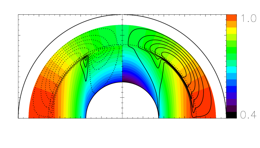
Figure 12: Normalized angular velocity ($\tilde{\Omega}/\Omega_{\rm eq}$) and streamlines solutions to equations (34) for an artificially weak stratification (see Figure 11), and for $f=10^{9}$ (corresponding to ${\rm E}_{\nu}=2\times 10^{-6}$ at the base of the convection zone). On the left, we show the solution with no-slip lower boundary conditions, and on the right the stress-free solution. Dotted lines represent clockwise flows, and solid lines counter-clockwise flows. In this calculation, the overshoot layer depth $\Delta$ was selected to be 0.01$R_{\odot}$, and $\Lambda=10$. The value of $D_{0}$ is irrelevant in this very weakly stratified simulation.

3.3 The stratified case

Let us now consider the case of a true solar stratification. Since $\lambda_{2}$ increases rapidly with depth beneath the convection zone (from 0 to about 10 in the case of the Sun), the radius at which $\lambda_{2}\simeq 1$ ($r_{1}$ for short) plays a special role: we expect the dynamics of the system to depend on the position of the lower boundary $r_{\rm in}$ compared with $r_{1}\simeq 0.55R_{\odot}$.

This is indeed observed in the simulations, as shown in Figure 13. If $r_{\rm in}>r_{1}$, then $\lambda_{2}<1$ everywhere in the modeled section of the radiative zone. In this case, the dynamics follow the scaling for the unstratified case, and depend on the nature of the lower boundary ($u_{r}\propto{\rm E}_{\nu}$ if the lower boundary is stress-free, and $u_{r}\propto{\rm E}_{\nu}^{1/2}$ if the lower boundary is no-slip). On the other hand, if $r_{\rm in}<r_{1}$ then the flows are strongly quenched by the stratification before they reach the lower boundary. As a result, the radial velocities scale with ${\rm E}_{\nu}/\lambda_{2}$ regardless of the applied boundary conditions.

The implications of this final result, namely the importance of the location of the stresses involved in breaking the Taylor-Proudman constraint in relation to the radius at which $\lambda_{2}\simeq 1$, are discussed in Section 4.3.

Figure 13: Vertical velocity (in units of $R_{\odot}\Omega_{\odot}$) in nine different simulations, at latitude $80^{\circ}$. The background stratification in each case is solar, but the position of the lower boundary is moved through the radiative zone from $0.65R_{\odot}$ to $0.35R_{\odot}$ and $0.1R_{\odot}$. The solid-line plots are for no-slip lower boundary conditions while the dotted lines are for stress-free lower boundary conditions. Three simulations are shown in each case: (from lowest to highest curve) for $f=10^{8}$, $f=10^{9}$ and $f=10^{10}$ corresponding to ${\rm E}_{\nu}=2\times 10^{-7}$ to ${\rm E}_{\nu}=2\times 10^{-5}$. The logarithmic scale clearly shows that $u_{r}$ scales with ${\rm E}_{\nu}$ in the radiative zone in the stress-free cases for all values of $r_{\rm in}$ while in the no-slip case, $r_{\rm in}$ scales with ${\rm E}_{\nu}$ if $r_{\rm in}<0.6$, as expected from Figure 10.

4 Implications of this work for solar and stellar mixing

4.1 Context for stellar mixing

The presence of mixing in stellar radiative zones has long been inferred from remaining discrepancies between models-without-mixing and observations (see Pinsonneault 1997 for a review). The most commonly used additional mixing source is convective overshoot, whereby strong convective plumes travel beyond the radiative–convective interface and cause intense but very localised (both in time and space) mixing events (Brummell, Clune & Toomre, 2002). The typical depth of the layer thus mixed, the “overshoot layer”, is assumed to be a small fraction of a pressure scaleheight in most stellar models.

A related phenomenon is wave-induced mixing (Schatzman, 1996). While most of the energy of the impact of a convective plume hitting the stably stratified fluid below is converted into local buoyancy mixing, a fraction goes into the excitation of a spectrum of gravity waves, which may then propagate much further into the radiative interior. Where and when the waves eventually cause mixing (either through mutual interactions, thermal dissipation or by transferring momentum to the large-scale flow) depends on a variety of factors. It has recently been argued that the interaction of the gravity waves with the local azimuthal velocity field (the differential rotation) would dominate the mixing process (Charbonnel & Talon 2005), although this statement is not valid unless the wave-spectrum is near-monochromatic. For the typically flatter wave spectra self-consistently generated by convection, wave-induced mixing has much more turbulent characteristics (Rogers, MacGregor & Glatzmaier 2008), and is again fairly localized below the convection zone.

Mixing induced by large-scale flows comes in two forms: turbulent mixing resulting from instabilities of the large-scale flows, and direct transport by the large-scale flows themselves. The former case is the dominant mechanism in the early stages of stellar evolution when the star is undergoing rapid internal angular-momentum “reshuffling” caused by external angular-momentum extraction (disk-locked and/or jet phase, early magnetic breaking phase). In these situations, regions of strong radial angular-velocity shear develop, which then become unstable and cause local turbulent mixing of both chemical species and angular momentum. Studies of these processes were initiated by the work of Endal & Sofia (1978). Later, Chaboyer & Zahn (1992) refined the analysis to consider the effect of stratification on the turbulence, and showed how this can differentially affect chemical mixing and angular-momentum mixing. Finally, Zahn (1992) proposed the first formalism which combines mixing by large-scale flows and mixing by (two-dimensional) turbulence. In addition to the flows driven by angular-momentum redistribution, he also considered flows driven by the local baroclinicity of the rotating star, and showed that their effect can be represented as a hyperdiffusion term in the angular velocity evolution equation. In a quasi-steady, uniformly rotating limit, the flows described are akin to a local Eddington-Sweet circulation. His formalism is used today in stellar evolution models with rotation (Maeder & Meynet, 2000).

In all cases described above, mixing is either localised near the base of the convection zone (overshoot, gravity-wave mixing), or significant only in very rapidly rotating stars (local Eddington-Sweet circulations) or stars which are undergoing major angular-momentum redistribution (during phases of gravitational contraction, spin-down, mass loss, etc..). In this paper, we have identified another potential cause of mixing, where the original energy source is the differential rotation in the stellar convective region: gyroscopic pumping (induced by the Coriolis force associated with the differential rotation, see McIntyre 2007) drives large-scale meridional flows which may – under the right circumstances – penetrate the radiative region and cause a global circulation.

This source of mixing is intrinsically non-local to the radiative zone. The simplest way of seeing this is to consider a thought-experiment where the radiative–convective interface is impermeable: as shown in Paper I, the amplitude of the meridional flows generated locally (i.e. below the interface) is then much smaller than the one calculated here. The origin of the flows is also clearly independent of the baroclinicity (since the same phenomenon is observed in the unstratified limit), although the flows themselves can be influenced by the stratification. This implies that they are not related to Eddington-Sweet flows. Finally, contrary to some of the other mixing sources listed above, the one described here does not rely on the system being out-of-equilibrium: it is an inherently quasi-steady phenomenon, implying that this process is an ideal candidate for “deep mixing” for stars on the Main Sequence.

The process together with the conditions under which strong mixing might occur, are now summarized and discussed.

4.2 Qualitative summary of our results

The differential rotation observed in stellar convective envelopes (e.g. Barnes et al. 2005) is thought to be maintained by anisotropic Reynolds stresses, arising from rotationally constrained convective eddies (Kippenhahn, 1963). The details of this particular process are beyond the scope of this study, but are the subject of current investigation by others (Kitchatinov & Rüdiger, 1993, 2005; Rempel, 2005). Instead, we have assumed here the simplest possible type of forcing which mimics the effect of convective Reynolds stresses in driving the system towards a differentially rotating state. Using this model, we then derive the expected mixing caused by large-scale meridional flows.

We first found that large-scale flows are indeed self-consistently driven by gyroscopic pumping in the convection zone, as expected (McIntyre, 2007). The amplitude of these flows within the convection zone scales roughly as

$$V_{\rm cz}\sim\tau R_{\star}(\Delta\Omega)\mbox{ , }$$ (39)

where $(\Delta\Omega)$ is the observed equator-to-pole differential rotation, $R_{\star}$ is the stellar radius, and $\tau$ is, as discussed in Section 2.2, related to the ratio of the convective turnover time divided by the rotation period. Note that for the Sun, with $(\Delta\Omega)\sim 0.1\Omega_{\odot}$, the typical amplitude of the corresponding meridional flows would be of the order of 200 $\tau$ m/s – which doesn’t seem too unreasonable given the observations of subsurface flows (Giles et al. 1997) and the typical values of $\tau$ in the solar convection zone (see Section 2.2).

Next, we studied how much mixing these flows might induce in the underlying radiative zone. In this quasi-steady formalism, we found that the magnitude of convection-zone-driven flows decays exponentially with depth below the radiative–convective interface on the lengthscale $l_{2}$, where $l_{2}=R_{\odot}/{\rm Pr}^{1/2}{\rm Ro}_{\rm rz}$, as determined in Section 2.4.2 (see also Gilman & Miesch, 2004 and Garaud & Brummell, 2008). This penetration corresponds (in the linear regime) to a so-called “thermo-viscous” mode. The limit $l_{2}\ll R_{\odot}$ corresponds to a strongly stratified limit, where the flow velocities are rapidly quenched beneath the convection zone. The limit $l_{2}\gg R_{\odot}$ corresponds to the weakly stratified case, where the thermo-viscous mode spans the whole radiative interior and the stratification has little effect on the flow. It is important to note that “weakly stratified” regions in this context can either correspond to regions with weak temperature stratification (small $\bar{N}$), or in rapid rotation, or with small Prandtl number – this distinction will be used later.

The amplitude of the flows upon entering the radiative zone $V_{\rm rz}$, together with $l_{2}$, uniquely define the global circulation timescale in the interior (roughly speaking, $l_{2}/V_{\rm rz}$). In the weakly stratified/rapidly rotating limit, we find that the fraction of the meridional mass flux pumped in the convection zone which is allowed to enter the radiative zone is strongly constrained by Taylor-Proudman’s theorem. This theorem, which holds when the pressure gradient and the Coriolis force are the two dominant forces and are therefore in balance, enforces the invariance of all components of the flow velocities along the rotation axis. Hence, flows which enter the radiative zone cannot return to the convection zone unless the Taylor-Proudman constraint is broken. However, additional stresses (such as Reynolds stresses, viscous stresses, magnetic stresses) are needed to break this constraint. As a result, two regimes may exist. If the (weakly stratified/rapidly rotating) radiative zone is in pure Taylor-Proudman balance, then the system adjusts itself, by adjusting the pressure field, in such a way as to ensure that the convection zone flows remain entirely within the convection zone. On the other hand, if there are other sources of stresses somewhere in the radiative zone to break the Taylor-Proudman balance, then significant large-scale mixing is possible since flows entering the radiative zone are allowed to return to the convection zone. Furthermore, the resulting meridional mass flux in the radiative zone depends rather sensitively on the nature of the mechanism which breaks the Taylor-Proudman constraint (see next section).

The strongly stratified/slowly rotating limit exhibits a very different behavior. Because of the strong buoyancy force, the Taylor-Proudman balance becomes irrelevant, the flows are exponentially suppressed, and the induced radiative zone mixing is independent of the lower boundary conditions. However, note that since $\bar{N}$ tends to 0 at a radiative–convective interface, there will always be a “weakly stratified” region in the vicinity of any convective zone. In that region the dynamics described in the previous paragraph apply.

4.3 Applications to the Sun and other stars

In the illustrative model studied here, the only stresses available to break the Taylor-Proudman constraint are viscous stresses, which are only significant within the thin Ekman layer located near an artificial impermeable inner boundary. We do not advocate that this is a particularly relevant mechanism for the Sun! However, it is a useful example of the sensitive dependence of the global circulation mass flux on the mechanism responsible for breaking the Taylor-Proudman constraint.

In the limit of weak stratification, we found that if the inner boundary is a stress-free boundary then the global turnover time within the radiative zone is the viscous timescale. This is because stress-free boundary conditions effectively suppress the Ekman layer. On the other hand if the boundary layer is no-slip, then the global mass flux through the radiative zone is equal to the mass flux allowed to return through the Ekman layer. In that case, and according to well-known Ekman layer dynamics, the overall turnover time within the bulk of the domain is the geometric mean of the viscous timescale and the rotation timescale ($1/{\rm E}_{\nu}^{1/2}\Omega_{\odot}$), which correspond to a few million years only.

Going beyond simple Ekman dynamics, a much more plausible related scenario for the solar interior was studied by Gough & McIntyre (1998). They considered the same mechanism for the generation of large-scale flows within the convection zone, studied how these flows down-well into the radiative zone and interact with an embedded large-scale primordial magnetic field. They showed that the field can prevent the flows from penetrating too deeply into the radiative zone, while the flows confine the field within the interior. In their model, this nonlinear interaction occurs in a thin thermo-magnetic diffusion layer, located somewhat below the radiative–convective interface. One can therefore see an emerging analogy with the dynamics discussed here: in the Gough & McIntyre model, the field does act as a somewhat impermeable barrier, and provides an efficient and elegant mechanism for breaking the Taylor-Proudman constraint within the radiative zone. The only significant difference is that the artificial Ekman layer is replaced by a more convincing thermo-magnetic diffusion layer: the mass flux allowed to down-well into the radiative zone, and mix its upper regions, is now controlled by a balance between the Coriolis force and magnetic stresses (instead of the viscous stresses). With this new balance, they find that the global turnover time for the circulation in the region between the base of the convection zone and the thermo-magnetic diffusion layer is of the order of a few tens of millions of years (which is still short compared with the nuclear evolution timescale).

This mixed region is the solar tachocline. By relating their model with observations, Gough & McIntyre were able to identify the position of the magnetic diffusion layer to be just at the base of the observed tachocline (around $0.68\pm 0.01R_{\odot}$, see Charbonneau et al. 1999). This turns out to be close enough to the base of the convection zone for the dynamics of the radiative region to be weakly-stratified in the sense used in this paper (see Figure 10 and Section 3.3) so that the meridional flows are indeed able to penetrate, and do so with “significant” amplitude (about $10^{-5}$ cm/s) down to the magnetic diffusion layer. However, it is rather interesting to note that the Gough & McIntyre model could not have worked had today’s tachocline been observed to be much thicker. It is also interesting to note that for younger, more rapidly rotating solar-type stars, a much larger region of the radiative zone can be considered “weakly stratified”, possibly leading to much deeper mixed regions if these stars also host a large-scale primordial field. The implications of these findings for Li burning, together with a few other interesting ideas, will be discussed in a future publication.

Appendix A: Ekman jump condition

Equation (2.3.2) provides the solution “far” from the lower boundary, in the bulk of the fluid. Let us refer to the limit of bulk solutions as $z\rightarrow 0$ as $\hat{u}_{\rm bulk}(0^{+})$ (and similarly for the other quantities). We now derive the Ekman solution close to the boundary, for the unstratified case. Let’s study the problem using the stream-function $\psi$ with

$$(\hat{u},\hat{v},\hat{w})=\left(\hat{u},\frac{{\rm d}\hat{\psi}}{{\rm d}z},-ik\hat{\psi}\right)\mbox{ . }$$ (1)

Moreover, let us assume that within the boundary layer, ${\rm d}\hat{\psi}/{\rm d}z\gg k\hat{\psi}$. The governing equations are then approximated by

$$-2\frac{{\rm d}\hat{\psi}}{{\rm d}z}=E_{\nu}\frac{{\rm d}^{2}\hat{u}}{{\rm d}z^{2}}\mbox{ , }$$

$$2\hat{u}=-ik\hat{p}+E_{\nu}\frac{{\rm d}^{3}\hat{\psi}}{{\rm d}z^{3}}\mbox{ , }$$

$$\frac{{\rm d}\hat{p}}{{\rm d}z}=-ikE_{\nu}\frac{{\rm d}^{2}\hat{\psi}}{{\rm d}z^{2}}\mbox{ , }$$ (2)

which simplify to

$$\frac{{\rm d}^{5}\hat{\psi}}{{\rm d}z^{5}}=-4\frac{{\rm d}\hat{\psi}}{{\rm d}z}\mbox{ , }$$ (3)

with solutions

$$\hat{\psi}(z)=\psi_{0}+\psi_{1}e^{\lambda_{3}}+\psi_{2}e^{-\lambda_{3}z}+\psi_{3}e^{\lambda_{4}z}+\psi_{4}e^{-\lambda_{4}z}\mbox{ , }$$

$$\hat{u}(z)=u_{0}-\frac{2}{E_{\nu}}\left[\frac{1}{\lambda_{3}}\psi_{1}e^{\lambda_{3}z}-\frac{1}{\lambda_{3}}\psi_{2}e^{-\lambda_{3}z}+\frac{1}{\lambda_{4}}\psi_{3}e^{\lambda_{4}z}-\frac{1}{\lambda_{4}}\psi_{4}e^{-\lambda_{4}z}\right]\mbox{ , }$$ (4)

where

$$\lambda_{3}=(1+i){\rm E}_{\nu}^{-1/2}\mbox{ , }\lambda_{4}=(1-i){\rm E}_{\nu}^{-1/2}\mbox{ . }$$ (5)

The growing exponentials are ignored to match the solution far from the boundary layer; it then becomes clear that $u_{0}=\hat{u}_{\rm bulk}(0^{+})$, while $-ik\psi_{0}=\hat{w}_{\rm bulk}(0^{+})$. Requiring no-slip, impermeable conditions at $z=0$ implies

$$\psi_{0}+\psi_{2}+\psi_{4}=0\mbox{ , }$$

$$\lambda_{3}\psi_{2}+\lambda_{4}\psi_{4}=0\mbox{ , }$$

$$u_{0}-\frac{2}{E_{\nu}}\left[-\frac{1}{\lambda_{3}}\psi_{2}-\frac{1}{\lambda_{4}}\psi_{4}\right]=0\mbox{ , }$$ (6)

which in turn implies

$$\psi_{4}=-\frac{\lambda_{3}}{\lambda_{4}}\psi_{2}\mbox{ , }$$

$$\psi_{2}=\frac{\lambda_{4}}{\lambda_{3}-\lambda_{4}}\psi_{0}\mbox{ , }$$

$$u_{0}=\frac{2}{E_{\nu}}\frac{\lambda_{3}+\lambda_{4}}{\lambda_{3}\lambda_{4}}\psi_{0}=2E_{\nu}^{-1/2}\psi_{0}\mbox{ . }$$ (7)

This last equation then uniquely relates the limit of the bulk solution $\hat{u}(0^{+})$ and $\hat{w}(0^{+})$ as $z\rightarrow 0$ as

$$\hat{u}_{\rm bulk}(0^{+})=\frac{2i}{k}E_{\nu}^{-1/2}\hat{w}_{\rm bulk}(0^{+})\mbox{ , }$$ (8)

yielding the standard Ekman jump condition.

Appendix B: Stratified stress-free solution

The boundary conditions discussed in Section 2.3.3 imply the following set of equations. At $z=0$, $\hat{w}=0$ and $\hat{u}_{z}=0$ (alternatively, $\hat{T}=0$):

$$0=u_{3}-u_{4}\mbox{ , }$$

$$0=ku_{1}-ku_{2}+\lambda_{2}u_{3}-\lambda_{2}u_{4}\mbox{ . }$$ (9)

At $z=1$: $\hat{w}=0$ and $\hat{T}=0$:

$$0=Ae^{1/\delta}+Be^{-1/\delta}-\frac{2iS}{k\Lambda}\mbox{ , }$$ (10)

$$0=T_{0}e^{k}+T_{1}e^{-k}\mbox{ . }$$ (11)

Finally, matching conditions on $\hat{w}$, $\hat{p}$, $\hat{T}$ and ${\rm d}\hat{T}/{\rm d}z$ at $z=h$:

$$-ikE_{\nu}\frac{k^{2}-\lambda_{2}^{2}}{\lambda_{2}}u_{3}\sinh(\lambda_{2}h)=Ae^{h/\delta}+Be^{-h/\delta}-\frac{2iS}{k\Lambda}\mbox{ , }$$

$$2u_{1}\cosh(kh)+2u_{3}\cosh(\lambda_{2}h)=U_{0}(h)+\frac{ik}{2}\delta\Lambda\left[Ae^{h/\delta}-Be^{-h/\delta}\right]\mbox{ , }$$

$$T_{0}e^{kh}+T_{1}e^{-kh}=-\frac{4}{ik{\rm Ro}_{\rm rz}^{2}}\left[ku_{1}\sinh(kh)+\lambda_{2}u_{3}\sinh(\lambda_{2}h)\right]\mbox{ , }$$

$$T_{0}e^{kh}-T_{1}e^{-kh}=-\frac{4}{ik^{2}{\rm Ro}_{\rm rz}^{2}}\left[k^{2}u_{1}\cosh(kh)+\lambda_{2}^{2}u_{3}\cosh(\lambda_{2}h)\right]\mbox{ , }$$ (12)

where $u_{4}$ and $u_{2}$ were already eliminated using equations (11). We now proceed to eliminate $A$, $B$, $T_{0}$ and $T_{1}$, which leaves two equations for $u_{1}$ and $u_{3}$:

$$2G\left[u_{1}\cosh(kh)+u_{3}\cosh(\lambda_{2}h)\right]-\delta\Lambda k^{2}E_{\nu}\frac{k^{2}-\lambda_{2}^{2}}{2\lambda_{2}}u_{3}\sinh(\lambda_{2}h)\mbox{ , }$$

$$\quad=\delta S\left(e^{(h-1)/\delta}(1-G)-1\right)+GU_{o}(h)\mbox{ , }$$

$$\left(F-1\right)ku_{1}\sinh(kh)+ku_{1}\cosh(kh)=-\frac{\lambda_{2}^{2}}{k}u_{3}\cosh(\lambda_{2}h)-\left(F-1\right)\lambda_{2}u_{3}\sinh(\lambda_{2}h)\mbox{ , }$$ (13)

where the functions $F(h,k)$ and $G(h,h)$ are geometric factors defined as

$$F(h,k)=\frac{2}{1-e^{2k(h-1)}}\mbox{ , }$$

$$G(h,k)=\frac{e^{(h-2)/\delta}-e^{-h/\delta}}{e^{(h-2)/\delta}+e^{-h/\delta}}\mbox{ . }$$ (14)

These equations form a linear system for $u_{1}$ and $u_{3}$ with

$$u_{1}=-Hu_{3}\mbox{ , }$$

$$u_{3}=\frac{\delta S\left(e^{(h-1)/\delta}(1-G)-1\right)+GU_{o}(h)}{2G\left[-H\cosh(kh)+\cosh(\lambda_{2}h)\right]-\delta\Lambda k^{2}E_{\nu}\frac{k^{2}-\lambda_{2}^{2}}{2\lambda_{2}}\sinh(\lambda_{2}h)}\mbox{ , }$$ (15)

and where the function $H(h,k,\lambda_{2})$ is given as

$$H(h,k,\lambda_{2})=\frac{\lambda_{2}}{k}\frac{\frac{\lambda_{2}}{k}\cosh(\lambda_{2}h)+\left(F-1\right)\sinh(\lambda_{2}h)}{\cosh(kh)+\left(F-1\right)\sinh(kh)}\mbox{ . }$$ (16)

These rather opaque solutions can be clarified a little by looking at the various relevant limits. For weakly stratified fluids $\lambda_{2}\rightarrow 0$. Then $H(h,k,\lambda_{2})=O(\lambda_{2}^{2})\rightarrow 0$, and so

$$u_{3}=\frac{\delta S\left(e^{(h-1)/\delta}(1-G)-1\right)+GU_{o}(h)}{2G-\delta\Lambda k^{4}E_{\nu}\frac{h}{2}}+O(\lambda^{2}_{2})\mbox{ . }$$ (17)

In the limit ${\rm E}_{\nu}\rightarrow 0$ this then becomes

$$u_{1}=O(\lambda_{2}^{2})\mbox{ , }$$

$$u_{3}=\frac{1}{2}\left[U_{o}(h)-\delta S\frac{1-\cosh((1-h)/\delta)}{\sinh((1-h)/\delta)}\right]\mbox{ . }$$ (18)

Folding this back into the original solution in the radiative zone then yields

$$\hat{w}(z)=-ik^{3}E_{\nu}u_{3}z=-\frac{ik^{3}E_{\nu}}{2}\left[U_{o}(h)-\delta S\frac{1-\cosh((1-h)/\delta)}{\sinh((1-h)/\delta)}\right]z\mbox{ , }$$ (19)

which is identical to equation (19).

In the opposite, strongly stratified limit, $\lambda_{2}\gg k$. Then we have instead

$$H(h,k,\lambda_{2})\simeq\frac{\lambda_{2}^{2}}{k^{2}}\frac{\cosh(\lambda_{2}h)}{\cosh(kh)+\left(F-1\right)\sinh(kh)}\mbox{ , }$$ (20)

so that this time $u_{3}=O(\lambda_{2}^{-2})\rightarrow 0$, and in the limit ${\rm E}_{\nu}\rightarrow 0$

$$u_{1}=\frac{1}{2\cosh(kh)}\left[U_{o}(h)-\delta S\frac{1-\cosh((1-h)/\delta)}{\sinh((1-h)/\delta)}\right]\mbox{ . }$$ (21)

Folding this back into the equation for $\hat{w}(z)$ in the radiative zone now yields

$$\hat{w}(z)=-\frac{ik^{3}{\rm E}_{\nu}}{2\lambda_{2}}\frac{\sinh(\lambda_{2}z)}{\cosh(\lambda_{2}h)}\left(1-\frac{\tanh(kh)}{\tanh(k(1-h))}\right)\left[U_{o}(h)-\delta S\frac{1-\cosh((1-h)/\delta)}{\sinh((1-h)/\delta)}\right]\mbox{ , }$$ (22)

therefore justifying the scaling discussed in 2.4.3.

References

- (1) Barnes, J.R., Collier Cameron, A., Donati, J.-F., James, D. J., Marsden, S. C., & Petit, P., 2005, MNRAS, 357, L1
- (2) Brummell, N. H., Clune, T. L., & Toomre, J., 2002, ApJ, 570, 825
- (3) Chaboyer, B. & Zahn, J.-P., 1992, A&A, 253, 173
- (4) Charbonneau, P., 2005, LRSP, 2, 2
- (5) Charbonnel, C. & Talon, S., 2005, Science, 309, 2189
- (6) Christensen-Dalsgaard, J., et al., 1996, Science, 272, 1286
- (7) Elliott, J. R. & Gough, D. O., 1999, ApJ, 516, 475
- (8) Endal, S. & Sofia, S., 1978, ApJ, 229, 279
-
(9)
Garaud, P., 2001, PhD Thesis
available from http://www.ams.ucsc.edu/pgaraud/ - (10) Garaud, P., 2007. in The Solar Tachocline, pp. 147–181, eds. Hughes, D. W., Rosner, R. & Weiss, CUP.
- (11) Garaud, P. & Brummell, N. H., 2008, ApJ, 674, 498
- (12) Garaud, P. & Garaud, J.-D., 2008, MNRAS, 391, 1239
- (13) Giles, P. M., Duvall, T. L., Jr., Scherrer, P. H. & Bogart, R. S, 1997, Nature, 390, 52
- (14) Gilman, P. A. & Miesch, M. S., 2004, ApJ, 611, 568
- (15) Gough, D. O. & McIntyre, M. E., 1998, Nature, 394, 755
- (16) Gough, D. O., 2007. in The Solar Tachocline, pp. 3–30, eds. Hughes, D. W., Rosner, R. & Weiss, CUP.
- (17) Kippenhahn, R., 1963, ApJ, 137, 664
- (18) Kitchatinov L. L. & Rüdiger, G., 1993, A&A, 276, 96
- (19) Kitchatinov L. L. & Rüdiger, G., 2005, Astr. Nachr., 326, 379
- (20) LaBonte, B. J. & Howard, R. F., 1982, Solar Phys., 80, 361
- (21) Maeder, A. & Meynet, G., 2000, ARA&A, 38, 143
- (22) McIntyre, M. E., 2007. in The Solar Tachocline, pp. 183-212, eds. Hughes, D. W., Rosner, R. & Weiss, CUP.
- (23) Pinsonneault, M., 1997, ARA&A, 35, 557
- (24) Rempel, M., 2005, ApJ, 622, 132
- (25) Rogers, T. M., MacGregor, K. B. & Glatzmaier, G. A., 2008, MNRAS, 387, 616
- (26) Rüdiger, G., 1989, in Differential rotation and stellar convection. Sun and the solar stars, Chapter 4. Publisher: Berlin, Akademie Verlag
- (27) Schatzman, E., 1996, J. Fluid Mech., 322, 355
- (28) Schou, J., et al., 1998, ApJ, 505, 390
- (29) Spiegel, E. A. & Bretherton, F. P., 1968, ApJ, 153, L77
- (30) Zahn, J.-P., 1992, A&A, 265, 115