Unified nonequilibrium dynamical theory for exchange bias and training effects

Abstract

We investigate the exchange bias and training effects in the FM/AF heterostructures using a unified Monte Carlo dynamical approach. This real dynamical method has been proved reliable and effective in simulating dynamical magnetization of nanoscale magnetic systems. The magnetization of the uncompensated AF layer is still open after the first field cycling is finished. Our simulated results show obvious shift of hysteresis loops (exchange bias) and cycling dependence of exchange bias (training effect) when the temperature is below 45 K. The exchange bias fields decrease with decreasing the cooling rate or increasing the temperature and the number of the field cycling. With the simulations, we show the exchange bias can be manipulated by controlling the cooling rate, the distributive width of the anisotropy energy, or the magnetic coupling constants. Essentially, these two effects can be explained on the basis of the microscopical coexistence of both reversible and irreversible moment reversals of the AF domains. Our simulated results are useful to really understand the magnetization dynamics of such magnetic heterostructures. This unified nonequilibrium dynamical method should be applicable to other exchange bias systems.

I Introduction

Usually, when the heterostructure consisting of coupled ferromagnetic (FM) and antiferromagnetic (AF) layers is cooled in field below the Neel temperature of its AF component, it shows the asymmetric magnetization c ; d ; e ; 6 ; 7 ; a , which is referred to as the exchange bias effect. Furthermore, the exchange bias field, defined as the average of the two coercive fields, is observed to decrease with increasing the number of the consecutive field cycling, which is referred to as the training effect5 . The exchange bias and training effects are very interesting and could be used in future spintronicsh ; i ; j and data storage. Usually, the FM layer is taken as a whole and the AF layer consists of many grains. The AF grain is small enough to consists of a single domain, and some uncompensated domains (or grains) may be formed by defects or impurities15 ; k ; 16 and couple with each other and with the FM domains. As the heterostructure is cooled to a low temperature, the uncompensated spins in the grains and domains become locked-in and prefer to a unidirection in the interface, thus contribute to the magnetization shift7 . Moreover, under the reversal of FM domains, the uncompensated grains or domains will be irreversibly reorganizedl ; m ; f ; g ; 4 and thus cause the training effect. The idea of domain states was corroborated in some Monte Carlo simulationsb . On the other hand, Hoffmann17 considered the biaxial anisotropy of the AF sublattices and solved it by variational method. Actual nonequilibrium dynamical properties of the magnetization are still waiting to be elucidated. It is highly desirable and needed to systematically investigate the two effects in a unified theory.

In this article we use a unified Monte Carlo dynamical approach10 to study the FM/AF heterostructure in order to investigate the exchange bias and training effect. Our simulated result shows the obvious shift of hysteresis loops and the cycling dependence of exchange bias. The magnetization of uncompensated AF layer is still open after the field cycling is finished. The exchange bias fields decrease with decreasing the cooling rate or increasing the temperature and the number of the field cycling. With the simulations, we shows the exchange bias can be manipulated by controlling the cooling rate, the distributive width of the anisotropy energy, or the magnetic coupling constants. Essentially, these two effects can be explained on the basis of the microscopically irreversible reversal of the AF domains. More detailed results will be presented in the following.

The remaining part of this paper is organized as follows. In next section we shall define our model and discuss our simulation method. In section III we shall present our simulated results and analysis. In section IV we shall discuss the microscopic mechanism for the phenomena in a unified way. Finally, we shall give our conclusion in section V.

II model and method

According to experimental observations18 , for both compensated and uncompensated AF layers the easy axis tends to form along external cooling field direction rather than later rotating field direction. In our model the AF layer consists of many AF domains, and the FM layer consists of one single domain. Assuming the cooling field is applied parallel to the AF/FM interface, then all the easy axes of AF and FM domains lie in the plane of the interface. The coupled bilayers of AF and FM domains are shown in the inset of Fig. 1(a). The rectangles of the white pattern represent the AF domains and the larger rectangle is the single FM domain. The AF domains couple to each other antiferromagnetically and the single FM domain couples to all the AF domains ferromagnetically. We define the $z$ axis along the common easy axis which lies in the interface plane. We apply the external field to saturate the magnetization of the FM layer along the $z$ axis.

For simplicity, we consider all the uncompensated spins in the AF domains are the same. We use $S^{\prime}\vec{s}_{i}$ to denote the spin vector of the $i$th AF domain and $S\vec{s}$ to denote that of the single FM domain, where $S^{\prime}$ and $S$ are the uncompensated spin values and FM spin respectively. Then we write the Hamiltonian of the bilayers in an external field as

$$H = -K_{u}(s^{z})^{2}-\sum_{i}k_{ui}(s^{z}_{i})^{2}-\vec{B}\cdot(\gamma^{\prime}\sum_{i}\vec{s}_{i}+\gamma\vec{s})$$ (1)

$$+J_{1}\sum_{i,j}\vec{s}_{i}\cdot\vec{s}_{j}-J_{2}\sum_{i}\vec{s}_{i}\cdot\vec{s}$$

where $\gamma^{\prime}=g\mu_{0}\mu_{B}S^{\prime}$ and $\gamma=g\mu_{0}\mu_{B}S$. The first and second terms represents the anisotropy of the FM domain and the AF ones, and $K_{u}$ and $k_{ui}$ are the corresponding anisotropy constants. The third term represents the Zeeman energy of the moments due to the applied external field. The fourth term represents the antiferromagnetic coupling among the AF domains. The last term represents the ferromagnetic coupling between the FM and AF domains.

Using $\theta_{i}$ and $\beta$ to describe the angles of the $i$-th AF moment and the FM moment deviating from the common easy axis, we can express the energies of the FM domain and the $i$-th AF as

$$H^{\mathrm{FM}}=-(J_{2}\sum_{i}s_{i}s+K_{u}\cos\beta+\gamma Bs)\cos\beta$$ (2)

and

$$H^{\mathrm{AF}}_{i}=(J_{1}s_{i}\sum_{j}s_{j}-J_{2}s_{i}s{}-k_{ui}\cos\theta_{i}-\gamma^{\prime}Bs_{i})\cos\theta_{i}$$ (3)

where both $s_{i}$ and $s$ are the scalars taking either 1 or -1. Thus for the $i$-th AF domain the energy increment is $\Delta E_{i}=k_{ui}\sin^{2}\theta_{i}-h_{i}(\cos\theta_{i}-1)$, where $h_{i}=(-J_{1}\sum_{j}s_{j}+J_{2}s+\gamma^{\prime}B)s_{i}$, and for the FM domain the energy increment is $\Delta E=K_{u}\sin^{2}\beta-h_{F}(\cos\beta-1)$, where $h_{F}=(J_{2}\sum_{i}s_{i}+\gamma B)s$. We can express $\Delta E$ and $\Delta E_{i}$ as10

$$\Delta E=K_{u}[(1+\frac{h_{F}}{2K_{u}})^{2}-(\cos\beta+\frac{h_{F}}{2K_{u}})^{2}]$$ (4)

and

$$\Delta E_{i}=k_{ui}[(1+\frac{h_{i}}{2k_{ui}})^{2}-(\cos\theta_{i}+\frac{h_{i}}{2k_{ui}})^{2}]$$ (5)

As a result, to reverse its moment, the the FM layer must overcomes a barrier $E_{b}^{F}=K_{u}(1+h_{F}/2K_{u})^{2}$ if $|h_{F}|\leq 2K_{u}$, or $2h_{F}$ if $h_{F}>2K_{u}$; and the $i$-th AF grain a barrier $E_{b}^{i}=k_{ui}(1+h_{i}/2k_{ui})^{2}$ if $|h_{i}|\leq 2k_{ui}$, or $2h_{i}$ if $h_{i}>2k_{ui}$. If the condition $h_{F}<-2K_{u}$ or $h_{i}<-2k_{ui}$ is satisfied, there is no barrier for the reversal.

Actually, for the distribution of the AF anisotropy energy we use a Gauss function, $f(k_{ui})=\exp[-(k_{ui}-k_{u})^{2}/\sigma^{2}]$, whose $\sigma$ and $k_{u}$ are set to 30.0 meV and 50.0 meV unless stated otherwise. The anisotropy energy of the FM domain is set 200.0 meV without losing main physics. Thus the reversal rate for a spin to reverse is $R=R_{0}e^{-E_{b}/k_{B}T}$, where $E_{b}$ is the energy barrier and $R_{0}$ is the characteristic frequency. In our simulations, $R_{0}$ is set to $1.0\times 10^{9}$/s. We adopt a square lattice for the AF domains and use $20\times 20$ as its size. Since we are only interested in the exchange bias and training effect at the nanoscale, the AF lattice is enough to capture main physics. Furthermore, we assume the AF domains have uniform moment 4.0 $\mu_{B}$ and the FM domain 2000 $\mu_{B}$. The coupling constant $J_{1}$ is set to 4.0 meV, and $J_{2}$ 8.0 meV. In our simulations the system is quenched from a high-enough temperature such as 610 K, at which the AF layer is paramagnetic, to a low-enough temperature such as 10 K. The magnetization and exchange bias fields are calculated at the low temperature 10 K unless the temperature is explicitly stated otherwise. The basic rate of changing temperature is $\nu_{0}$= 50 K/s. The field sweeping rate is set to 0.5 T/s with the basic increment 0.1 T for each simulation step.

III Simulated Results and analysis

At first, we let the AF/FM bilayers relax under a magnetic field of 5.0 T at a high temperature 610 K. This temperature is enough to make both the FM layer and the AF layer remain paramagnetic. When the temperature decreases, the average magnetization values of the two layers increases. The external field makes the average magnetization of the FM layer have a large increase below 600 K, and reach nearly to the saturated value at 500 K. When the temperature becomes lower than 60 K, the average magnetization of the AF layer looks like that of an antiferromagnet under an applied field and is dependent on the cooling rate $\nu$. Then, we further cool the bilayers under the same field. After the temperature reaches down to 10 K, we start to change the field while keeping the temperature unchanged. The field decreases from 5.0 T to -10.0 T and then increases back to 5.0 T for the first hysteresis. Repeating the field cycling, we will make the second hysteresis loop. The simulated results are shown in Fig. 1.

Figure 1: The first two hysteresis loops of the FM (a) and AF (b) layer at 10 K. The inset in (a) shows the AF/FM bilayers. The hysteresis loop is obtained by changing the field in the order of P1-P2-P3-P4-P1.

As shown in Fig. 1(a), the origin of the first hysteresis is clearly shifted in the negative field direction and shows the exchange bias. The exchange bias field is defined as $H_{E}=(H_{cl}+H_{cr})/2$, where $H_{cl}$ and $H_{cr}$ is the coercivity of the left and right branches. The left branch of the second hysteresis moves towards the positive direction, but the right branches of the first two loops almost coincide with each other. Actually, any further loop almost does no difference in the right branch from the second hysteresis. The shift of the second loop clearly demonstrates that the bilayers magnetization depends on the cycling history, which is known as training effect. Fig. 1(b) shows the magnetization of the AF layer, which drops largely and opens widely due to the irreversible reversal of the AF domains after the first field cycling is finished. The subsequent magnetization is more smooth but still not closed, indicating the continuing cycling dependence of exchange bias. This is consistent with other Monte Carlo simulationsb .

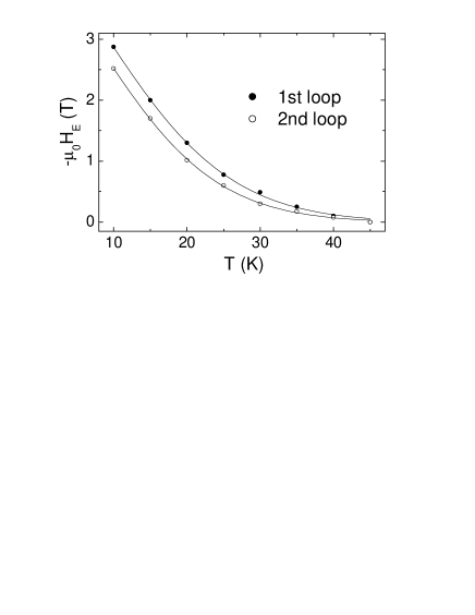
Figure 2: Temperature dependence of the exchange bias fields for the first two loops. The exchange bias field is calculated at a given temperature after the system is cooled from 610 K to the temperature value. The lines are the fitting curves in terms of the simple function defined in Eq. (6).

We study the effect of the temperature $T$ on the exchange bias field, $H_{E}$, for different loops. Our simulated exchange bias fields as functions of $T$ for the first two loops are shown in Fig. 2. For both of the two curves, the data can be fitted by the simple function

$$-\mu_{0}H_{E}=a_{1}e^{-(T/T_{1})^{b_{1}}}$$ (6)

where $a_{1}$, $T_{1}$, and $b_{1}$ are fitting parameters. For the fitting in Fig. 2, the parameters $a_{1}$, $T_{1}$, and $b_{1}$ takes 4.26 T, 17.95 K, and 1.58 for the first loop, and 3.94 T, 16.66 K, and 1.59 for the second loop. Our results are consistent with experimental observation that the exchange bias field decreases with increasing temperature 19 ; k ; n .

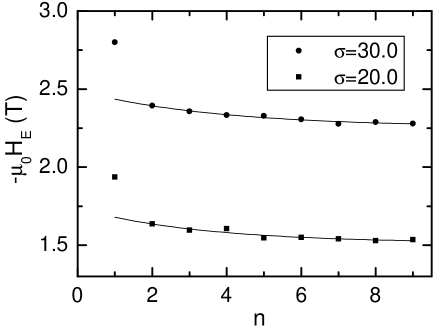
Figure 3: The loop-number dependence of the exchange bias fields for the Gaussian width $\sigma$=30.0 and 20.0 meV. The temperature is 10 K. All the data except for $n=1$ can be well fitted by a simple function $-\mu_{0}H_{E}(n)=a_{2}\rho^{n}+b_{2}$.

The exchange bias field is dependent on the field cycling number $n$. Our simulated result from $n$=1 to $n$=9 is shown in Fig. 3. Here, the temperature is kept at 10 K, and $\sigma$ is set to 20.0 and 30.0 meV. For both of the curves in Fig. 3, the data points excepts of $n=1$ are well fitted by the simple function $-\mu_{0}H_{E}(n)=a_{2}\rho^{n}+b_{2}$, where $a_{2}$, $b_{2}$, and $\rho$ are the fitting parameters, taking 0.23 T, 2.26 T, and 0.76 for $\sigma=30.0$ meV, and 0.22 T, 1.51 T, and 0.74 for $\sigma=20.0$ meV. The value of $-\mu_{0}H_{E}(1)$ usually is substantially above the extrapolation of the other $-\mu_{0}H_{E}(n)$ ($n>1$). These simulated results are in good agreement with experimental observation5 .

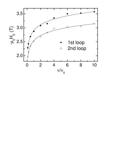
Figure 4: The cooling-rate dependence of the exchange bias fields for the first two loops. The lines are the fitting curves in terms of Eq. (7).

Since the training effect reflects the non-equilibrium dynamical magnetization which is caused by the irreversible reversal of meta-stable domains formed during quenching, the quenching rate must affect the exchange bias field. By changing the cooling rate $\nu$, we study the exchange bias field as the function of quenching rate $\nu$. The result is shown in Fig. 4. For both of the loops, the data be well fitted by

$$-\mu_{0}H_{E}=a_{3}\ln(b_{3}\frac{\nu}{\nu_{0}}+1)$$ (7)

where $a_{3}$ and $b_{3}$ are 0.292 T and 20847 for the first loop, and 0.262 T and 16248 for the second loop. The exchange bias field at 10 K increases logarithmically with increasing the quenching rate.

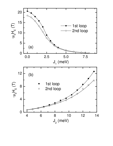
Figure 5: The exchange bias fields as functions of the coupling-constants $J_{1}$ (a) and $J_{2}$ (b) for the first two loops.

Figure 6: The exchange bias field as a function of the Gaussian width $\sigma$ for the first two loops.

It is interesting to investigate the dependence of the exchange bias field on the coupling constants $J_{1}$ and $J_{2}$. The simulated results are shown in Fig. 5. As shown in Fig. 5(a), the exchange bias field decreases with increasing $J_{1}$. The training effect is nearly unchanged when $J_{1}$ changes from 0 to 2meV, but diminishes to zero quickly with increasing $J_{1}$ from 2meV. When $J_{1}$ is larger than 6 meV, the exchange bias field already becomes very small and the training effect is actually zero. In contrast, the $J_{2}$ data points in Fig. 5(b) can be well fitted by the simple function $-\mu_{0}H_{E}=a_{4}(\exp(J_{2}/b_{4})-1)$, where $a_{4}$ and $b_{4}$ are the fitting parameters, taking 0.44 T and 4.01 meV for the first loop, and 0.51 T and 4.49 meV for the second loop. It is clearly shown that the exchange bias field increases exponentially as $J_{2}$ increases. Both of the the exchange bias field and the training effect can be enhanced by decreasing $J_{1}$ and increasing $J_{2}$, or by increasing $J_{2}/J_{1}$. This is consistent with experimental trendp . In Fig. 6 we shows how the distributive width $\sigma$ of the AF anisotropy affects the exchange bias fields. Clearly the exchange bias field increases with $\sigma$, and so does the training effect. Experimentally, the width can be increased by the additional nonmagnetic impurities and the enhanced roughness of the AF crystalline phases. This implies that the rougher the AF crystalline phases are, the larger the exchange bias and training effect. Our result reveals that the exchange bias field is determined by both the coupling constants and the distributive width of the AF domain anisotropy. These are useful to completely understand the phenomenonp ; o .

IV Trends and microscopic mechanism

After being cooled down to the low temperature, the AF layer has a non-zero net FM moment $M_{A}$ due to the driving of both the field and the FM layer. Assuming there are $N_{A}$ AF domains, on average we have the moments in part of all the $N_{A}$ AF domains aligning parallel although they are coupled with AF interactions. The exchange bias field is determined by the effective moment $M_{A}$, the difference of $M_{A}$ between the first two loops determines the training effect. Naturally, both the exchange bias field and the training effect increase with increasing $J_{2}$ and with decreasing $J_{1}$, as shown in Fig. 5. Actually, small $J_{1}$ does not affect the effects, but larger $J_{1}$ than 2meV is harmful to the effects at 10 K. In addition, it is easily understood that $M_{A}$ decreases with increasing the temperature $T$. As a result, both the exchange bias field and the training effect decrease with increasing $T$, as shown in Fig. 2. The exponential description in Eq. (6) reflects the fact that moment reversals are thermally activated. It is reasonable that both the exchange bias field and the training effect increase with increasing the cooling rate $\nu$, as shown in Fig. 4. This is mainly because the average magnetization of the AF layer increases with $\nu$ when the temperature is below 50 K. When the cooling rate approaches to zero, both the exchange bias field and the training effect should be zero. In another word, our results should approach to those of corresponding equilibrium systems when the cooling rate $\nu$ approaches to zero.

As shown in Fig. 6, both the exchange bias field and the training effect are nearly zero when the distributive width $\sigma$ of the AF anisotropy energy is smaller than 15 meV, but they increase substantially with increasing $\sigma$ for $\sigma>15$ meV. This means that the effects are dependent on a wide distribution of the anisotropy energy. This can be understood in terms of the changing of the energy barriers with the external field. From P1 to P2 in Fig. 1(a), the effective barrier of the FM layer decreases but is still high enough to avoid the reversal, but meanwhile, more and more spins of the AF domains are reversed due to their lower energy barriers. At the point P2, the FM moment is reversed with the help of the field and the reversing of the AF domains. Anyway, some AF domains with high energy barriers have their moments unchanged, even after the FM layer has been reversed, and thus there is a net average moment of the AF domains parallel to the moment of the FM layer. This net average moment increases with the distributive width $\sigma$. This explains the increasing of the exchange bias field and training effect with increasing $\sigma$. The more the field cycling loops, the longer the time. Actually, this is similar to reducing the cooling rate $\nu$ in effect. As a result, the exchange bias field decreases with increasing the number of the field cycling. The turning point of the time scale causes the largest drop happens between the first loops.

V Conclusion

In summary, we use a unified Monte Carlo dynamical approach10 to study the FM/AF heterostructure in order to investigate the exchange bias and training effect. The magnetization of uncompensated AF layer is still open after the first field cycling is finished. Our simulated result shows the obvious shift of hysteresis loops (exchange bias) and the cycling dependence of exchange bias (training effect). The exchange bias fields decrease with decreasing the cooling rate or increasing the temperature and the number of the field cycling. With the simulations, we show the exchange bias can be manipulated by controlling the cooling rate, the distributive width of the anisotropy energy, or the magnetic coupling constants. Essentially, these two effects can be explained on the basis of the microscopical coexistence of both reversible and irreversible moment reversals of the AF domains. Our simulated results are useful to really understand the magnetization dynamics of such magnetic heterostructures which should be important for spintronic device and magnetic recording media p ; o ; 20 . This unified nonequilibrium dynamical method should be applicable to other exchange bias systems.

- (1) S. Bruck, G. Schutz, E. Goering, X. S. Ji, and K. M. Krishnan, Phys. Rev. Lett. 101, 126402 (2008).
- (2) M. Gruyters and D. Schmitz, Phys. Rev. Lett. 100, 077205 (2008).
- (3) Y. Ijiri, T. C. Schulthess, J. A. Borchers, P. J. van der Zaag, and R. W. Erwin, Phys. Rev. Lett. 99, 147201 (2007).
- (4) J. Eisenmenger, Z. P. Li, W. A. A. Macedo, and I. K. Schuller, Phys. Rev. Lett. 94, 057203 (2005).
- (5) S. Brems, D. Buntinx, K. Temst, and C. V. Haesendonck, Phys. Rev. Lett. 95, 157202 (2005).
- (6) J. Nogues and I. K. Schuller, J. Magn. Magn. Mater. 192, 203 (1999).
- (7) A. Hochstrat, C. Binek, and W. Kleemann, Phys. Rev. B 66, 092409 (2002).
- (8) T. Zhao, A. Scholl, F. Zavaliche, K. Lee, M. Barry, A. Doran , M. P. Cruz, Y. H. Chu, C. ederer, N. A. Spaldin, R. R. Das, D. M. Kim, S. H. Baek, C. B. Eom, and R. Ramesh, Nat. Mater. 5, 823 (2006); R. Ramesh and N. A. Spaldin, Nat. Mater. 6, 21 (2007).
- (9) V. Laukhin, V. Skumryev, X. Mart, D. Hrabovsky, F. Sanchez, M. V. Cuenca, C. Ferrater, M. Varela, U. Luders, J. F. Bobo, and J. Fontcuberta, Phys. Rev. Lett. 97, 227201 (2006).
- (10) P. Borisov, A. Hochstrat, X. Chen, W. Kleemann, and C. Binek, Phys. Rev. Lett. 94, 117203 (2005).
- (11) P. Miltenyi, M. Gierlings, J. Keller, B. Beschoten, and G. Guntherodt, Phys. Rev. Lett. 84, 4224 (2000).
- (12) J. I. Hong, T. Leo, D. J. Smith, and A. E. Berkowitz, Phys. Rev. Lett. 96, 117204 (2006).
- (13) F. U. Hillebrecht, H. Ohldag, N. B. Weber, C. Bethke, and U. Mick, Phys. Rev. Lett. 86, 3419 (2001).
- (14) M. Bode, E. Y. Vedmedenko, K. V. Bergmann, A. Kubetzka, P. Ferriani, S. Heinze, and R. Wiesendanger, Nat. Mater. 5, 477 (2006).
- (15) W. Kuch, L. I. Chelaru , F. Offi, J. Wang, M. Kotsugi, and J. Kirschner, Nat. Mater. 5, 128 (2006).
- (16) F. Nolting, A. Scholl, J. Stohr, J. W. Seo, J. Fompeyrine, H. Siegwart, J. P. Locquet, S. Anders, J. Luning, E. E. Fullerton, M. F. Toney, M. R. Scheinfein, and H. A. Padmore, Nature (London) 405, 767 (2000).
- (17) X. P. Qiu, D. Z. Yang, S. M. Zhou, R. Chantrell, K. O. Grady, U. Nowak, J. Du, X. J. Bai, and L. Sun, Phys. Rev. Lett. 101, 147207 (2008).
- (18) T. Hauet, J. A. Borchers, P. Mangin, Y. Henry, and S. Mangin, Phys. Rev. Lett. 96, 067207 (2006).
- (19) U. Nowak, K. D. Usadel, J. Keller, P. Miltenyi, B. Beschoten, and G. Guntherodt, Phys. Rev. B 66, 014430 (2002).
- (20) A. Hoffmann, Phys. Rev. Lett. 93, 097203 (2004).
- (21) Y. Li and B.-G. Liu, Phys. Rev. B 73, 174418 (2006); Phys. Rev. Lett. 96, 217201 (2006); B.-G. Liu, K.-C. Zhang, and Y. Li, Front. Phys. China 2, 424 (2007).
- (22) W. Zhu, L. Seve, R. Sears, B. Sinkovic, and S. S. P. Parkin, Phys. Rev. Lett. 86, 5389 (2001).
- (23) M. Gruyters, Phys. Rev. Lett. 95, 077204 (2005).
- (24) V. K. Valev, M. Gruyters, A. Kirilyuk, and T. Rasing, Phys. Rev. Lett. 96, 067206 (2006).
- (25) J. Camarero, J. Sort, A. Hoffmann, J. M. G. Martin, B. Dieny, R. Miranda and J. Nogues, Phys. Rev. Lett. 95, 057204 (2005).
- (26) S. Brems, K. Temst, and C. V. Haesendonck, Phys. Rev. Lett. 99, 067201 (2007).
- (27) V. Skumryev, S. Stoyanov, Y. Zhang, G. Hadjipanayis, G. Dominique, and J. Nogues, Nature (London). 423, 850 (2003).