On Interband Pairing in Multiorbital Systems

Abstract

The discovery of high-$T_{c}$ superconductivity in the pnictides, materials with a Fermi surface determined by several bands, highlights the need to understand how superconductivity arises in multiband systems. In this effort, using symmetry considerations and mean-field approximations, we discuss how strong hybridization among orbitals may lead to both intra and interband pairing, and we present calculations of the spectral functions to guide the experimental search for this kind of state.

I Introduction

Iron-based high-$T_{c}$ superconductorsKamihara:2008p932 ; chen1 ; chen2 ; wen ; chen3 ; ren1 ; 55 ; ren2 have a complex Fermi surface that is determined by several bands, an effect resulting from the hybridization of the $3d$ orbitals of iron.first ; Singh:2008p1736 ; xu ; cao ; fang2 Band structure calculations have shown that the bands that define the two hole pockets around the $\Gamma$ point have mostly $d_{xz}$ and $d_{yz}$ character, while the two electron pockets around the M point have $d_{xz}$, $d_{yz}$, and a smaller amount of $d_{xy}$ contributions.plee ; first ; Singh:2008p1736 ; xu ; cao ; fang2 For this reason it is important to understand superconductivity in multiorbital systems in general terms.

Among the first to address this complex problem several years ago were Suhl et al.Suhl using a model consisting of two orbitals, one $s$ and one $d$, that did not hybridize with each other. Thus, in this case each band was determined by one single orbital. They showed that BCS pairingBCS could occur in each band and, since in the most general case the electron-phonon interaction would have different strengths for electrons in the different bands, it was proposed that two different superconducting gaps could arise. Almost 50 years were needed to observe experimental evidence of this phenomenon. In 2001, superconductivity with $T_{c}=39$ K was observed in MgB₂.akimitsu Despite the high-$T_{c}$, it became clear that the BCS mechanismLouie was at play and for the first time two different superconducting gaps were observed.Wang2001179 ; PhysRevLett.87.047001 ; PhysRevLett.87.167003 ; PhysRevLett.87.137005 ; PhysRevLett.87.177008 ; PhysRevLett.87.157002 ; PhysRevLett.87.177006 As shown in Ref. Louie, , the Fermi surface (FS) is determined by two bands: the $\pi$ band formed by the $p_{z}$ orbitals of B, and the $\sigma$ band constituted by a linear combination of the $p_{x}$ and $p_{y}$ B-orbitals. Although three orbitals determine the FS, it is interesting to notice that only two different BCS gaps are observed. This occurs because two of the three orbitals hybridize with each other and determine one single band, which couples strongly to the lattice phonons. This opens a large superconducting gap on the $\sigma$ FS. The other orbital, $p_{z}$, does not hybridize and forms the $\pi$ band that couples weakly to the lattice phonons determining a second, smaller, superconducting gap at the FS of the $\pi$ band. Thus, the number of different gaps that can arise in a multiorbital system is related to the degree of hybridization among the orbitals. Also note that in this early effort interband hopping of pairs of electrons belonging to the same band was included but the possibility of interband pairing, i.e., pairs formed by electrons belonging to two different bands, was not considered.

In this paper, the subject of superconductivity in multiorbital systems is revisited, in particular to shed light on the possible symmetry of the pairing operator of the pnictides superconductors. The motivation is that the pairing operators that have been discussed the most thus farkuroki ; Mazin:2008p1695 ; FCZhang ; han ; korshunov ; Baskaran:2008p832 ; plee ; yildirim ; Si:2008p1561 ; yao ; xu2 ; stratos assume that only intraband pairing should occur, namely the two electrons of the Cooper pair belong to the same band.dolgov However, numerical simulationsours performed on a two-orbital modelscalapino ; ours ; moreo for the pnictides favor an interorbital pairing operator that, when transformed to the band representation, results not only in intraband pairing but it includes interband pairing as well.moreo For the pnictides, interband hopping of pairs formed between electrons in the same band is often denoted as “Interband Superconductivity”.dolgov The situation discussed in the present paper is different and involves Cooper pairs where the two electrons come from two different bands, which we will call “Interband pairing”. Using symmetry arguments and mean-field approximations, the plausibility and physical meaning of such an interband pairing in multiorbital systems will be discussed.

Interband pairing has previously been addressed in the context of Quantum Chromodynamics (QCD) and cold atoms,PhysRevLett.90.047002 ; PhysRevLett.91.032001 heavy fermions,khomskii cuprateskheli , and BCS superconductivity.kumar In the case of heavy fermions, it was argued that interband pairing could occur if two Fermi surfaces arising from different bands are very close to one other,khomskii while in QCD and cold atoms it was presented as a possibility for the case of sufficiently strong attractive pairing interactions, or for weaker attractions among particles with very different masses.PhysRevLett.90.047002 ; PhysRevLett.91.032001 As it will be discussed for a simple model in Sec. III, three different regimes, shown schematically in Fig. 1, can result from a purely interband pairing as a function of the strength of the pairing potential $g$: (1) a normal regime where the ground state is not superconducting (namely in purely interband pairing an infinitesimal attraction does not lead to superconductivity), (2) an exotic superconducting “breached” regime where gaps open at the normal Fermi surfaces while new Fermi surfaces defining regions containing unpaired electrons are created, and (3) a superconducting regime resembling BCS states, at large attractive coupling.rong

Figure 1: Schematic representation of the three regimes that can arise as a function of the strength $g$ of an interband pairing attraction. The label “normal” denotes a non-superconducting state. The case “breached” is an exotic regime with superconductivity and gaps, coexisting with Fermi surfaces (or several nodes) and electrons that do not pair. “BCS” is the large attraction region, where the ground state resembles that of a BCS superconductor and all electrons participate in the pairing.

The paper is organized as follows. In Sec. II, the general form of pairing operators in multiorbital systems will be presented, remarking how the symmetry is determined by the spatial and the orbital characteristics of the operator. The interorbital pairing operator with $B_{2g}$ symmetry obtained numerically in a two-orbital model for the pnictides is discussed, emphasizing that this operator presents a mixture of intra and interband pairing in the band representation. In Sec. III, a simple toy model with pure interband pairing attraction is introduced. This simplified model is discussed in order to illustrate the effects of interband pairing on observables, such as the occupation number and the spectral functions $A({\bf k},\omega)$. The stability of the interband paired state is also discussed. The occupation number, spectral functions, and the stability of the $B_{2g}$ pairing state are the subject of Sec. IV which is directly related to the physics of pnictides, while Sec. V is devoted to the conclusions.

II Pairing Operators in Multiorbital Models

In single-orbital models, the symmetry of a spin-singlet pairing state is completely determined by the properties of its spatial form factor. More specifically, the pairing operator will have the form:

$$\Delta({\bf k})=f({\bf k)}(c_{{\bf k},\uparrow}c_{{\bf-k},\downarrow}-c_{{\bf k},\downarrow}c_{{\bf-k},\uparrow}),$$ (1)

where $c_{{\bf k},\sigma}$ destroys an electron with momentum ${\bf k}$ and spin projection $\sigma$ and $f({\bf k})$ is the form factor that transforms according to one of the irreducible representations of the crystal’s symmetry group. Thus, $f({\bf k})$ determines the symmetry of the operator. These form factors depend on the lattice geometry and generally they may be very complex. However, in materials with short pair coherence lengths, such as the high-$T_{c}$ cuprates, the assumption that the two particles that form the pair can be very close to one other is usually made. The Cu-oxide planes in the cuprates have the symmetry properties of the $D_{4h}$ group and the case $f({\bf k})=\cos k_{x}-\cos k_{y}$, which transforms according to the irreducible representation $B_{1g}$, provides the well-known $d$-wave symmetry pairing.

In multiorbital systems, on the other hand, a spin singlet pairing operator will have both spatial and orbital degrees of freedom and it will be given by

$$\Delta({\bf k})=f({\bf k)}\tau_{\alpha,\beta}(d_{{\bf k},\alpha,\uparrow}d_{{\bf-k},\beta,\downarrow}-d_{{\bf k},\alpha,\downarrow}d_{{\bf-k},\beta,\uparrow}),$$ (2)

where $d_{{\bf k},\alpha,\sigma}$ destroys an electron with momentum ${\bf k}$, in orbital $\alpha$, and with spin projection $\sigma$, $f({\bf k})$ is the spatial form factor as indicated above, and $\tau_{\alpha,\beta}$ is a matrix in the space spanned by the orbitals involved. The dimension of $\tau$ is equal to the number of orbitals that are considered to be of relevance. In this case, notice that the symmetry of the pairing operator would in general be determined by the product of the symmetry properties of $f({\bf k)}$ and the symmetry of the orbital contribution $\tau_{\alpha,\beta}$. Only if $\tau_{\alpha,\beta}$ is the identity matrix do the orbital contribution become trivial, because the identity matrix transforms according to $A_{1g}$. Thus, this is the only case where $f({\bf k})$ fully determines the symmetry of the pairing operator, as in the single-orbital example.

The minimum model for the pnictides considers the two orbitals $d_{xz}$ and $d_{yz}$, which are strongly hybridized.ours ; scalapino All the possible pairing operators, up to nearest-neighbor distance, that are allowed by the lattice and orbital symmetries have been already calculated.wang ; shi ; 2orbitals ; wan ; zhou ; goswami Numerical simulations performed on the two-orbital model suggest that the favored pairing operator at intermediate couplings, where the state is both magnetic and metallic, ours ; moreo has symmetry $B_{2g}$ and is given by Eq. (2) with $f({\bf k)}=(\cos k_{x}+\cos k_{y})$, which transforms according to $A_{1g}$, and $\tau=\sigma_{1}$ which transforms according to $B_{2g}$ wan (where $\sigma_{i}$ are Pauli matrices). Thus, the non-trivial symmetry under rotations arises from the orbital portion of the operator. This pairing operator has been studied at the mean-field level in Ref. moreo, . In the orbital representation, the Bogoliubov-de Gennes Hamiltonian matrix is given by:

$$H_{\rm MF}=\left(\begin{array}[]{cccc}\xi_{xx}&\xi_{xy}&0&\Delta_{\bf k}\\ \xi_{xy}&\xi_{yy}&\Delta_{\bf k}&0\\ 0&\Delta_{\bf k}&-\xi_{xx}&-\xi_{xy}\\ \Delta_{\bf k}&0&-\xi_{xy}&-\xi_{yy}\end{array}\right),$$ (3)

with

$$\xi_{xx} = -2t_{2}\cos k_{x}-2t_{1}\cos k_{y}-4t_{3}\cos k_{x}\cos k_{y}-\mu,$$

$$\xi_{yy} = -2t_{1}\cos k_{x}-2t_{2}\cos k_{y}-4t_{3}\cos k_{x}\cos k_{y}-\mu,$$

$$\xi_{xy} = -4t_{4}\sin k_{x}\sin k_{y},$$ (4)

and

$$\Delta_{\bf k}=V(\cos k_{x}+\cos k_{y}),$$ (5)

where $V=V_{0}\Delta$, with $V_{0}$ being the strength of the pairing interaction and $\Delta$ the mean-field parameter obtained by minimizing the energy. Since the two orbitals are hybridized via $\xi_{xy}$, in the band representation the Hamiltonian matrix becomes:

$$H^{\prime}_{\rm MF}=\left(\begin{array}[]{cccc}\epsilon_{1}&0&V_{B}&V_{A}\\ 0&\epsilon_{2}&-V_{A}&V_{B}\\ V_{B}&-V_{A}&-\epsilon_{2}&0\\ V_{A}&V_{B}&0&-\epsilon_{1}\end{array}\right),$$ (6)

where $V_{A}$ and $V_{B}$ are given by

$$V_{A}=2u({\bf k})v({\bf k})\Delta_{\bf k},\\$$ (7)

$$V_{B}=(v({\bf k})^{2}-u({\bf k})^{2})\Delta_{\bf k},$$ (8)

and $u({\bf k})$ and $v({\bf k})$ are the elements of the change of basis matrix $U$ given by

$$U=\left(\begin{array}[]{cccc}u({\bf k})&v({\bf k})&0&0\\ v({\bf k})&-u({\bf k})&0&0\\ 0&0&v({\bf k})&u({\bf k})\\ 0&0&-u({\bf k})&v({\bf k})\end{array}\right),$$ (9)

with $U^{-1}=U^{T}$. Remember that $V_{A}$ and $V_{B}$, are functions of the momentum ${\bf k}$, and $u({\bf k})^{2}+v({\bf k})^{2}=1$. Thus, it is clear that in the band representation, in addition to the intraband pairing given by $V_{A}$, there is also interband pairing given by $V_{B}$. Among pairing operators compatible with the symmetry of the model, the ones that do not lead to interband pairing not only cannot mix orbitals, but have to contain $\tau=\sigma_{0}$, i.e., the identity matrix.moreo One example for such an operator would be the $s_{\pm}$ pairing.kuroki ; Mazin:2008p1695 ; korshunov ; parker

The discussion above describes general properties of hybridized multi-orbital systems. If the orbitals are hybridized, but not related to one another by symmetry, there is no reason to expect that the coupling between the electrons in each orbital, and the interaction that produces the pairing, will have the same strength for all the orbitals and lead to a unit matrix in the orbital sector. Then, it is expected that interband pairing will arise in general and, thus, it is important to understand its consequences, providing the main motivation for the present manuscript.

III Interband Pairing

III.1 Generic properties

III.1.1 Model and non-interacting limit

To address qualitatively the issue of interband pairing, postponing the matters of stability to the next subsection (Sec. III.2), let us consider the following two-bands simplified model with interband pairing:

$$H_{\bf k}=\sum_{\alpha,\sigma}\epsilon_{\alpha}({\bf k})c^{\dagger}_{{\bf k},\alpha,\sigma}c_{{\bf k},\alpha,\sigma}+V\sum_{\alpha\neq\beta}(c^{\dagger}_{{\bf k},\alpha,\uparrow}c^{\dagger}_{-{\bf k},\beta,\downarrow}+h.c.),$$ (10)

where $\alpha,\beta,=1,2$ label two bands that are not hybridized, $\sigma$ is the spin projection, and for simplicity

$$\epsilon_{\alpha}({\bf k})={-{\bf k}^{2}\over{2m_{\alpha}}}+C,$$ (11)

which gives parabolic bands that are degenerate at ${\bf k}=0$ with energy $C$, and with a chemical potential $\mu=0$. This can be considered as a crude representation of the two hole-pocket bands around the $\Gamma$ point in the pnictides, but more importantly presents a simple toy model where the effects of interband pairing can be studied. As before, the parameter $V=V_{0}\Delta$ is the product of an attractive potential $V_{0}$ between electrons in the two different bands and a mean-field parameter $\Delta$ determined by minimizing the total energy. The band dispersion without the interaction is presented in the inset of Fig. 2.

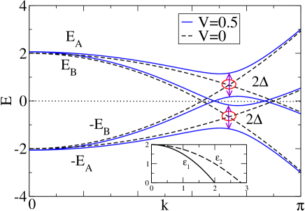
Figure 2: (Color online) Mean-field band dispersion for the model defined by Eq. (10), for the indicated values of $V$ (defined in the text) as a function of the momentum $k=\sqrt{k_{x}^{2}+k_{y}^{2}}$. The case shown is for $m_{1}=1$, $m_{2}=2$, and $C=2$. Inset: Non-interacting band dispersion for the same parameters.

The Bogoliubov-de Gennes matrix expressed in the basis expanded by $B_{12}=\{c^{\dagger}_{{\bf k},1,\uparrow},c_{-{\bf k},2,\downarrow},c^{\dagger}_{{\bf k},2,\uparrow},c_{-{\bf k},1,\downarrow}\}$ has the form:

$$H=\left(\begin{array}[]{cccc}\epsilon_{1}&V&0&0\\ V&-\epsilon_{2}&0&0\\ 0&0&\epsilon_{2}&V\\ 0&0&V&-\epsilon_{1}\end{array}\right).$$ (12)

This matrix can be diagonalized becoming

$$H_{D}=\left(\begin{array}[]{cccc}E_{A}&0&0&0\\ 0&-E_{B}&0&0\\ 0&0&E_{B}&0\\ 0&0&0&-E_{A}\end{array}\right),$$ (13)

in the basis expanded by $B_{AB}=\{\gamma^{\dagger}_{{\bf k},{\rm A},\uparrow},\gamma_{-{\bf k},{\rm B},\downarrow},\gamma^{\dagger}_{{\bf k},{\rm B},\uparrow},\gamma_{-{\bf k},{\rm A},\downarrow}\}$ and the change-of-basis matrix is given by

$$U=\left(\begin{array}[]{cccc}u_{\bf k}&v_{\bf k}&0&0\\ -v_{\bf k}&u_{\bf k}&0&0\\ 0&0&u_{\bf k}&v_{\bf k}\\ 0&0&-v_{\bf k}&u_{\bf k}\end{array}\right),$$ (14)

with $u_{\bf k}^{2}+v_{\bf k}^{2}=1$.

The four energy eigenvalues are

$$E_{i}({\bf k})=\pm\left[{(\epsilon_{1}-\epsilon_{2})\over{2}}\pm\sqrt{({\epsilon_{1}+\epsilon_{2}\over{2}})^{2}+V^{2}}\right],$$ (15)

where the first positive (negative) sign corresponds to the eigenvalues of the upper (lower) block, labeled $E_{A}$ and $-E_{B}$ ($E_{B}$ and $-E_{A}$) in Eq. (13) and in Fig. 2. The second sign differentiates between the two solutions in each block. Figure 2 shows the eigenvalues for $V=0$ and $V=0.5$. When $V=0$, then $E_{A}=\epsilon_{2}$ and $E_{B}=\epsilon_{1}$, the two bands define two circular Fermi surfaces with radius $k_{F1}$ and $k_{F2}$ where they cross the chemical potential ($\mu=0$). This is illustrated schematically in Fig. 3.

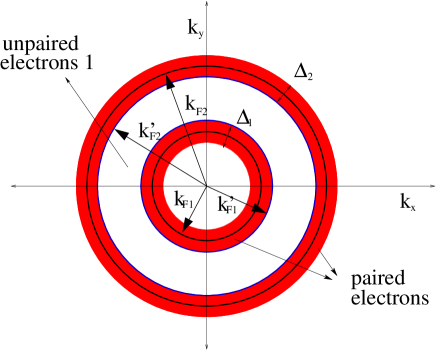
Figure 3: (Color online) Schematic diagram of the FS determined by the two parabolic bands of the simple model used in Sec. III. $k_{F1}$ and $k_{F2}$ indicate the Fermi momentum of the two bands when $V=0$, while $k^{\prime}_{F1}$ and $k^{\prime}_{F2}$ indicate the position of the Fermi momenta for the case of a finite but small pairing potential. The shaded rings indicate the regions with width $\Delta_{1}$ and $\Delta_{2}$ in momentum space where electrons can pair. The white region in between the rings contains unpaired electrons in band 1.

Notice that number operators can be defined in the two bases that are being considered here, i.e. $B_{12}$ and $B_{AB}$, which of course become equivalent when $V$=0. Thus, in the basis $B_{12}$ the number operator is,

$$n_{\alpha}({\bf k})=\sum_{\sigma}c^{\dagger}_{{\bf k},\alpha,\sigma}c_{{\bf k},\alpha,\sigma},$$ (16)

while in basis $B_{AB}$ the number operator is ($I$=A,B)

$$n_{I}({\bf k})=\sum_{\sigma}\gamma^{\dagger}_{{\bf k},{\rm I},\sigma}\gamma_{{\bf k},{\rm I},\sigma}.$$ (17)

The total electronic occupation of the system is given by

$$n({\bf k})=\sum_{\alpha}n_{\alpha}({\bf k})=\sum_{I}n_{I}({\bf k}).$$ (18)

Then, for $V=0$ we find that $n({\bf k})=0$ for $|{\bf k}|\leq|{\bf k}_{F1}|$, $n({\bf k})=2$ for $|{\bf k}_{F1}|<|{\bf k}|<|{\bf k}_{F2}|$ since in this region $n_{1}({\bf k})=n_{A}({\bf k})=2$ while $n_{2}({\bf k})=n_{\bf B}({\bf k})=0$, and finally $n({\bf k})=4$ for $|{\bf k}|>|{\bf k}_{F2}|$ since both orbitals are totally filled with electrons. These results are represented by the dashed lines in Fig. 4.

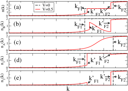
Figure 4: (Color online) Mean-field state population as a function of momentum along the diagonal $k_{x}=k_{y}$ for (a) the whole system; (b) band B, (c) band A; (d) orbital 1; and (e) orbital 2 for the indicated values of the pairing potential $V$, and $m_{1}=1$, $m_{2}=2$, and $C=2$.

III.1.2 Weak attraction

In the nontrivial case of $V$ different from zero, the bands $\pm E_{A}$ and $\pm E_{B}$ result from the hybridization of the $\epsilon_{1}$ and $\epsilon_{2}$ bands due to $V$. It is interesting to observe that an internal gap opens at the crossing of bands $E_{A}$ with $-E_{B}$ $above$ the chemical potential and between $E_{B}$ and $-E_{A}$ $below$ the chemical potential, as indicated with circles in Fig. 2 where results for $V=0.5$ are displayed. These are very important differences with respect to conventional BCS calculations were all the action is restricted to the original Fermi surfaces: for multiorbital models, gaps can open in other portions of the band structure as well.

While the $\pm E_{A}$ bands are separated by a gap, the bands $\pm E_{B}$ still cross the chemical potential determining two Fermi surfaces at $k^{\prime}_{F1}>k_{F1}$ and at $k^{\prime}_{F2}<k_{F2}$, even in this pairing state (again, this is different from the one-orbital pairing standard BCS ideas). The new Fermi surfaces are shown schematically in Fig. 3: the interior FS has expanded and the exterior one has contracted. In fact, it will be shown below that the effect of $V$ is to try to equalize the two Fermi surfaces, as this pairing attraction grows in magnitude. Calculating $n({\bf k})$ we observe that $n({\bf k})=4v_{\bf k}^{2}$ for $k<k^{\prime}_{F1}$ and $k>k^{\prime}_{F2}$, where $v_{\bf k}$ is the element of the change-of-basis matrix in Eq. (14). This agrees with the BCS expression for $n({\bf k})$ but it jumps discontinuously to $n({\bf k})=2$ for $k^{\prime}_{F1}<k<k^{\prime}_{F2}$. Such a result is shown by the solid lines in Fig. 4(a). The jumps indicate the existence of the two Fermi surfaces, which are here present even in the paired state. Thus, some electrons in the region in between the two Fermi surfaces may behave like normal unpaired electrons.

A better understanding of the electronic behavior can be achieved by studying the electronic density in the two bases $B_{AB}$ and $B_{12}$. We find that $n_{A}({\bf k})=2v_{\bf k}^{2}$, as shown in Fig. 4(c), which is the standard BCS behavior in agreement with the fact that bands $\pm E_{A}$ are separated by a gap. Thus, all the electrons in this band participate in the pairing and they do not have a FS. On the other hand, it can be shown that $n_{B}({\bf k})=n_{A}({\bf k})=2v_{\bf k}^{2}$ for $k<k^{\prime}_{F1}$ and $k>k^{\prime}_{F2}$, but for $k^{\prime}_{F1}<k<k^{\prime}_{F2}$ there is a discontinuous change of behavior to $n_{B}({\bf k})=u^{2}_{\bf k}=1-v^{2}_{\bf k}$ [Fig. 4(b)]. Thus, the Fermi surfaces are determined by electrons in the band $E_{B}$. However, note that in this region $n_{A}({\bf k})$ is an increasing function of $|{\bf k}|$ while $n_{B}({\bf k})$ is a decreasing function of $|{\bf k}|$ which satisfies $n_{A}({\bf k})+n_{B}({\bf k})=2$ for all $|{\bf k}|$.

This behavior can be better understood by calculating the (photoemission) spectral functions $A({\bf k},\omega)$, which allow us to obtain $n({\bf k})=\int_{-\infty}^{\mu=0}A({\bf k},\omega)d\omega$.

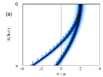
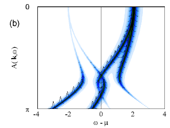
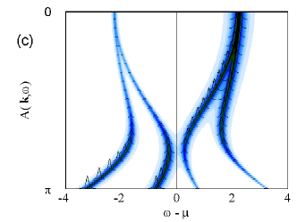
Figure 5: (Color online) (a) Spectral functions $A({\bf k},\omega)$ for the non-interacting case, $V=0$. (b) Same as (a) but for $V=0.5$. Note that there are still Fermi surfaces in this intermediate coupling case, namely gaps open far from the chemical potential but not at the Fermi level. (c) Same as (a) but for $V=1.0$. The presence of a gap for all the momenta shown is now clear.

In the non-interacting case, shown in Fig. 5(a), the spectral function shows two peaks, corresponding to the two bands $\epsilon_{1}$ and $\epsilon_{2}$, for each value of $|{\bf k}|$. This is the expectation for free electrons in a non-interacting multiorbital system. The two non-interacting FS’s are located where each band passes across the chemical potential.

When the pairing interaction becomes finite, the spectral function develops four peaks for each value of $|{\bf k}|$ as it can be observed in Fig. 5(b) for $V=0.5$. This is also the expected result since the BCS interaction generates a “shadow” or Bogoliubov band for each band present in the non-interacting system. For example, close to $|{\bf k}|=0$ the bands $E_{A}$ and $E_{B}$ have almost all the spectral weight, given by $u_{\bf k}^{2}$ which is very close to 1 in this region, and follow a dispersion similar to the non-interacting bands $\epsilon_{1}$ and $\epsilon_{2}$, while the bands $-E_{A}$ and $-E_{B}$ appear with very small spectral weight given by $v_{\bf k}^{2}=1-u^{2}_{\bf k}$. The latter are the Bogoliubov or “shadow” bands. These shadow bands appear above the chemical potential for large values of $|{\bf k}|$, as expected.

But what happens in the intermediate region $k^{\prime}_{F1}<k<k^{\prime}_{F2}$? We see that the band $E_{B}$ crosses with $-E_{B}$ at $k^{\prime}_{F1}$ determining a FS. Most of the spectral weight below the chemical potential belongs to the band $-E_{B}$ which contains the unpaired electrons but the band $-E_{A}$ has appreciable shadow spectral weight indicating that there are also some paired electronic population as indicated in Figs. 4(b) and (c). As $k$ increases, spectral weight is transferred continuously from $-E_{B}$ to $-E_{A}$, behavior associated with the internal gap opened by the pairing interaction, so that when $k$ approaches $k^{\prime}_{F2}$ most of the spectral weight below the chemical potential is in $-E_{A}$, paired electrons, and $-E_{B}$, unpaired electrons, has shadow spectral weight as seen in Figs. 4(b) and (c). At $k=k^{\prime}_{F2}$ the second FS is determined by the crossing of $\pm E_{B}$ at the chemical potential indicated by the sudden jump in $n_{B}$. Thus, the unpaired electrons in this region coexist with paired electrons and the spectral functions do not resemble the non-interacting ones.

It is also illuminating to analyze what happens with $n({\bf k})$ in the basis $B_{12}$. While $n_{1}({\bf k})=n_{2}({\bf k})=2v^{2}_{\bf k}$ in the regions where there are no unpaired electrons, we find discontinuities associated with Fermi surfaces in the two distributions that are given by $n_{2}({\bf k})=0$ and $n_{1}({\bf k})=2$ for $k^{\prime}_{F1}<k<k^{\prime}_{F2}$ [Figs. 4(d,e)]. This indicates that the pairing interaction $V$ has been able to promote some electrons from above to below $k_{F2}$ in orbital 2. Also, electrons have been transferred from their original location in orbital 1, in the neighborhood of $k_{F2}$ and above $k_{F1}$, to both orbitals 1 and 2 around $k_{F1}$. These are the electrons in 1 and 2 that have become paired (the pairing is indicated by the shadowed circular regions in Fig. 3). But the interaction was not strong enough to provide pairing partners to all the extra electrons originally in orbital 1 and, thus, they have been left unpaired in between the two paired regions, as indicated in Fig. 3.

Thus, the interband pairing attraction creates pairs of electrons belonging to different orbitals within an interval $\Delta_{k_{Fi}}$ around each of the two original Fermi surfaces. The width of the pairing region increases with $V$. The pairing partners are obtained by promoting electrons with momentum $k\approx k_{F2}$ and $k\approx k_{F1}$ in both orbitals and by moving electrons from the more populated to the less populated orbital. This creates the conditions to pair electrons near both Fermi surfaces. The electrons in band 1 that could not find promoted partners remain unpaired. Whether this state is stable or not depends, of course, on the balance between kinetic and pairing energies, which will be discussed in Sec. III.2.

III.1.3 Strong attraction

As the interaction $V$ increases further, the number of unpaired electrons is reduced. This means that $k^{\prime}_{F1}$ and $k^{\prime}_{F2}$ become closer to each other making the size of the intermediate region with unpaired electrons in Fig. 3 smaller. Eventually, the two momenta become the same $k^{\prime}_{F1}=k^{\prime}_{F2}$ for $V=0.71$, and for $V>0.71$ the region with unpaired electrons vanishes and a full gap opens in the system whose physics now resembles BCS, except for the fact that the pairs are constituted by electrons from different orbitals. The electronic population of the system in such a case, e.g. at $V=1.0$, is presented in Fig. 6 and the corresponding spectral functions are shown in Fig. 5(c). It can be shown that now $n_{1}({\bf k})=n_{2}({\bf k})$ for all values of $k$ and all the particles around the two noninteracting Fermi surfaces now participate in the pairing. The spectral functions show four peaks, i.e. Bogoliubov bands for all values of $k$, as it can be observed in Fig. 5(c).

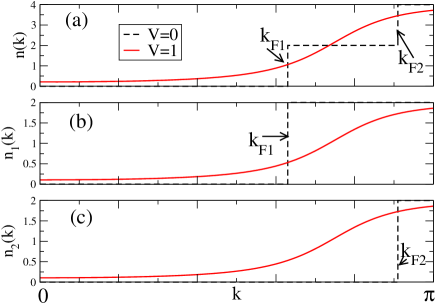
Figure 6: (Color online) Mean-field state population as a function of the momentum (main diagonal) for (a) the whole system, (b) band 1, and (c) band 2 for the indicated values of the pairing potential $V$, and for $m_{1}=1$, $m_{2}=2$, and $C=2$. The case $V=1.0$ illustrates the “strong” pairing attraction regime where gaps open in the original Fermi surface.

Thus, notice that while band 1 contained more electrons than band 2 for $V=0$ [see Figs. 6(b) and (c)], the interband pairing mechanism transfers electrons from one band to the other so that both bands have the same number of electrons in the superconducting state. Consequently, the smaller FS expands and the larger one shrinks. Then, when the pairing becomes strong enough, the two Fermi surfaces become equalized and no unpaired electrons remain. Whether this situation can be achieved will depend on the strength of the interaction and the energy balance, as discussed in the next subsection.

If the two non-interacting Fermi surfaces are very close to each other in momentum space, even relatively weak pairing interaction could effectively be strong enough to make the interband pairing resemble BCS pairing as in the case of large $V$ in the present example.

III.2 Stability of the interband paired state

III.2.1 The case without intraband pairing

As discussed in the Introduction, the possibility of interband pairing has been previously discussed in the context of QCD and cold atomic matter. Similar effects on the FS as found in the present study were described, although the physics was different because in the QCD context each band contained different kinds of particles and the pairing was thus not able to promote particles from the majority to the minority band.PhysRevLett.90.047002 ; PhysRevLett.91.032001 The issue of stability was explored in the QCD framework, and it was found that a purely interband paired state could be stabilized for pairing attractions $above$ a certain cut-off value, which could become very small for a large difference between the masses of the two paired species.PhysRevLett.90.047002 ; PhysRevLett.91.032001

In the case of our model, however, we have found (see below) that the purely interband-paired state only becomes stable when the attraction is sufficiently strong that no unpaired particles are left, i.e. when the two shaded regions overlap and the unpaired region in Fig. 3 vanishes. This means that, although the pairs would be formed by electrons in different orbitals, the physics would be analogous to BCS. A gap will be opened in the full Fermi surface of the simple model studied here.

In order to study the issue of stability, let us assume that the interaction term responsible for the interband attraction is given by

$$H_{\rm attr}={1\over{N}}\sum_{{\bf k,k^{\prime}},\alpha}V_{\bf k,k^{\prime}}c^{\dagger}_{{\bf k},\alpha,\uparrow}c^{\dagger}_{{\bf-k},-\alpha,\downarrow}c_{{\bf-k^{\prime}},-\alpha,\downarrow}c_{{\bf k^{\prime}},\alpha,\uparrow},$$ (19)

where $V_{\bf k,k^{\prime}}=-V_{0}$ and $N$ is the number of sites. Performing the standard mean-field approximation: $b_{\bf k^{\prime}}=\langle c_{{\bf-k^{\prime}},-\alpha,\downarrow}c_{{\bf k^{\prime}},\alpha,\uparrow}\rangle$ and $b^{\dagger}_{\bf k}=\langle c^{\dagger}_{{\bf k},\alpha,\uparrow}c^{\dagger}_{{\bf-k},-\alpha,\downarrow}\rangle$ and making the substitution $c^{\dagger}_{{\bf k},\alpha,\uparrow}c^{\dagger}_{{\bf-k},-\alpha,\downarrow}=b^{\dagger}_{\bf k}+(c^{\dagger}_{{\bf k},\alpha,\uparrow}c^{\dagger}_{{\bf-k},-\alpha,\downarrow}-b^{\dagger}_{\bf k})$ (and an analogous substitution for the product of annihilation operators), the mean-field results are obtained. As usual, the fluctuations around the average given by $(c^{\dagger}_{{\bf k},\alpha,\uparrow}c^{\dagger}_{{\bf-k},-\alpha,\downarrow}-b^{\dagger}_{\bf k})$ are assumed to be small. Defining $\Delta={1\over{N}}\sum_{\bf k}b_{\bf k}={1\over{N}}\sum_{\bf k}b^{\dagger}_{\bf k}$ we obtain the following mean-field Hamiltonian:

$$H_{\rm MF}=\sum_{\alpha,\sigma}\epsilon_{\alpha}({\bf k})c^{\dagger}_{{\bf k},\alpha,\sigma}c_{{\bf k},\alpha,\sigma}$$

$$-V_{0}\Delta\sum_{{\bf k},\alpha\neq\beta}(c^{\dagger}_{{\bf k},\alpha,\uparrow}c^{\dagger}_{{\bf-k},\beta,\downarrow}+h.c.)+2V_{0}\Delta^{2}N.$$ (20)

Equation (12) can be recovered by defining $-V_{0}\Delta=V$, and disregarding the constant last term of Eq. (20). We can calculate the total energy $E_{\rm MF}$ for Eq. (20) as a function of $V=V_{0}\Delta$. If for a given $V\neq 0$ the energy has a minimum, this indicates that the interband-paired state is stable. Note that having a term linear in $\Delta$ in Eq.(20) is not sufficient to conclude the appearance of a superconducting state at small $\Delta$, since the sign of the coefficient of the linear term can change sign with $V$. A similar situation occurs for the magnetic state of undoped pnictides: a finite Hubbard $U$ must be reached to stabilize the “striped” state rong . Returning to superconductivity, there are two regions of interest: (i) $0<V<0.71$, which corresponds to the case in which two Fermi surfaces are present in the paired state; (ii) $V>0.71$, which corresponds to the fully gapped case. In Fig. 7(a), $E_{\rm MF}/N$ vs. $V$ is shown for different values of $V_{0}$. It can be observed that a second minimum develops for $V_{0}>2$ and it becomes stable for $V_{0}>3$. The minimum always occurs for $V>0.71$ which means that it corresponds to the case in which there are no unpaired electrons in the system. The results shown in the figure are robust in the sense that changes in the values of $m_{1}$, $m_{2}$ or the chemical potential were not found to stabilize the state with unpaired electrons. Thus, in this respect an attraction that is only interband can only lead to a stable superconducting state in the strong attraction region.

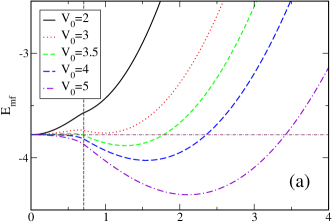
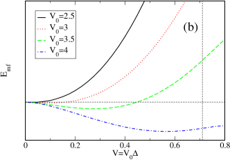
Figure 7: (Color online)(a) Mean-field energy Eq. (20) per site vs. $V=V_{0}\Delta$ for different values of $V_{0}$. The case $V=0.71$ is indicated with dashed lines: it separates the regions corresponding to nodal and nodeless states. (b) Mean-field energy (Eq. 20) per site with intraband pairing with strength $V_{0}/2$ vs. $V=V_{0}\Delta$, for different values of $V_{0}$.

III.2.2 Stability when both inter and intraband pairing coexist

The results of the previous paragraphs may seem negative with respect to the relevance of the “intermediate” state with simultaneous coexistence of pairing and Fermi surfaces. However, as pointed out in Sec. II, most of the pairing operators allowed by the lattice and orbital symmetry in the pnictides are characterized by a mixture of both intra and interband pairing. Thus, it is important to consider such a situation in our simple model as well. In the case of the $B_{2g}$ pairing operator, Eqs. (6), (7), and (8) indicate that the pairing is purely interband only for $k_{x}=0$ or $\pi$ and $k_{y}=0$ or $\pi$, because $V_{A}=0$ along these lines. Thus, let us now consider our simple model in a Brillouin zone (BZ) defined by $-\pi<k_{x},k_{y},\leq\pi$ and with the addition of intraband pairing with intensity $V_{0}/2$ that is vanishing for $k_{x}=0$ or $\pi$ and $k_{y}=0$ or $\pi$, i.e., the pairing is purely interband only along those directions. The energy bands now behave as in Fig. 2 only along $(0,0)-(\pi,0)$ and $(0,0)-(0,\pi)$, while the dispersion along any other direction is shown in Fig. 8 for $V=0$ and $V=0.5$.

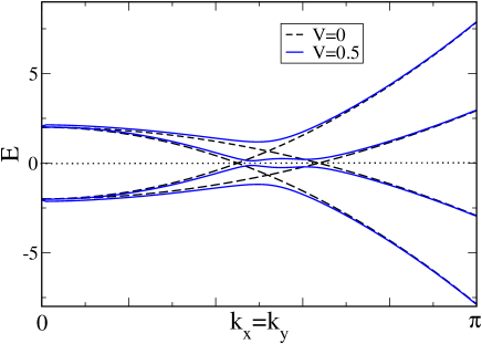
Figure 8: (Color online) Mean-field band dispersion for the model given by Eq. (10) (along the main diagonal) for the indicated values of the pairing potential $V$, with the addition of an intraband pairing with strength $V_{0}/2$, as described in the text.

Performing the mean-field approximation similarly as explained above, we have found that the superconducting state now becomes stable on both sides of the original critical value $V=0.71$. Figure 7(b) shows that the pairing state is stabilized for $V_{0}>2.5$ but the value of $\Delta$ where the minimum is located is such that $V<0.71$ and, thus, two nodes will be present along the $x$ and $y$ axes. Increasing the value of $V_{0}$, the minimum eventually occurs for $V>0.71$. For these larger values of $V_{0}$, there would consequently be no nodes.

Then, in this section it has been shown using a simple model that the interorbital paired state can become stable if the attraction $V_{0}$ is sufficiently strong. In this case, it is the nodeless case that is stable even for purely interband attraction. In addition, the very interesting novel phase with coexisting nodes and unpaired electrons in the majority band also requires intraband pairing to be stable, with strength similar to that of the interband, at least in parts of the BZ.

IV The interorbital $B_{2g}$ Pairing Operator

In the previous section, a simple model was presented, both with exclusively interband pairing and with both inter and intraband pairing, and it was found that the intraband pairing stabilizes the state with a mixture of superconductivity and metallicity. As mentioned in the Introduction, it is expected that in the most general cases the pairing operators allowed by the symmetry of the lattice and of the orbitals will, in the band representation, have both intra and interorbital pairing. Thus, now we will present and discuss, at the mean field level, the occupation number and the spectral functions for the pairing operator obtained from the numerical study of the two-orbital model for the superconducting state of the pnictides introduced in Sec. II.

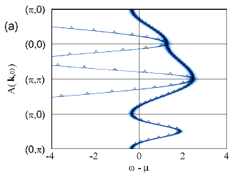
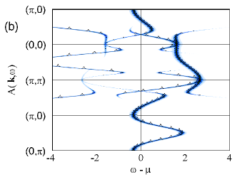
Figure 9: (Color online) (a) One-particle spectral function for the two-orbital model Eq. (3), with vanishing pairing interaction $V=0$. Parameters: $t_{1}=1.3$, $t_{2}=-1$, $t_{3}=t_{4}=-0.85$, $\mu=1.54$. (b) Same as (a) but for $V=0.5$.

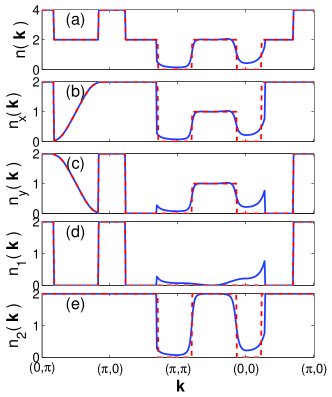
Figure 10: (Color online) (a) Total occupation number $n({\bf k})$ for the two-orbital model Eq. (3) with pairing interaction $V=0.5$ (continuous lines) and $V=0$ (dashed lines). Parameters: $t_{1}=1.3$, $t_{2}=-1$, $t_{3}=t_{4}=-0.85$, $\mu=1.54$. (b) Same as (a) but for the orbital $d_{xz}$. (c) Same as (a) but for the orbital $d_{yz}$. (d) Same as (a) but for band 1. (e) Same as (a) but for band 2.

IV.1 Non-interacting limit

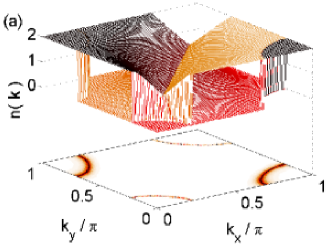
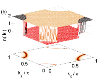
Figure 11: (Color online) (a) Occupation number $n({\bf k})$ for the two-orbital model Eq. (3) without pairing interaction for the orbital $d_{xz}$ (orange/light) and the orbital $d_{yz}$ (red/dark). The ‘floor’ indicates the FS in red. (b) Same as (a) but for band 1 (orange/light) and band 2 (red/dark)

Let us start with the non-interacting case in which $V=0$. The spectral functions along high-symmetry directions in momentum space are presented in Fig. 9 and, as expected, they reproduce the non-interacting band dispersion. We also show the total occupation number $n({\bf k})$ along the same directions [dashed lines in Fig. 10(a)], as well as the occupation number for each orbital $n_{x}({\bf k})$ [dashed lines in panel (b)] and $n_{y}({\bf k})$ [dashed lines in panel (c)] and the orbital occupation in the quadrant of the first BZ defined by $0\leq k_{x},k_{y}\leq\pi$ in Fig. 11(a). It is clear that the electron-like and hole-like Fermi surfaces are determined by an admixture of the two orbitals.

On the other hand, in the band representation, band 1 determines the electron pockets while band 2 forms the hole pockets as it can be seen from the behavior of $n_{1}({\bf k})$ and $n_{2}({\bf k})$ (indicated by the dashed lines in panels (d) and (e) of Fig. 10) and by the light (orange) and dark (red) surfaces in Fig. 11(b) where the FS is also indicated. It is clear that the electronic occupation of band 1 is smaller than the electronic population of band 2, so that unpaired electrons would be expected to belong predominantly to band 1, as in the simple model of the previous Sec. III. It is interesting to notice that in the orbital representation, on the other hand, the electrons are equally distributed among the $xz$ and $yz$ $3d$ orbitals.

IV.2 Nonzero pairing

Let us discuss what occurs when the pairing interaction becomes nonzero. To simplify the discussion, define the following points in momentum space: $X=(\pi,0)$, $Y=(0,\pi)$, $\Gamma=(0,0)$, and $M=(\pi,\pi)$. As remarked in Ref. moreo, , the $B_{2g}$ pairing operator always has nodes along the $X-Y$ direction because the spatial form factor $f({\bf k})=\cos k_{x}+\cos k_{y}$ vanishes along that line. But, as soon as $V$ is finite, a gap opens along the $\Gamma-M$ direction [notice that along this direction the pairing is purely intraband since in Eq. (6), $v^{2}=u^{2}$ and thus $V_{B}=0$ in Eq. (8)]. Along $\Gamma-X$, $\Gamma-Y$, $X-M$, and $Y-M$ nodes associated to the different number of electrons in band 1 and band 2 remain [notice that along these directions the pairing is purely interband since $V_{A}=0$ because Eq. (3) and Eq. (6) become identical to one other]. When the pairing interaction $V$ becomes strong enough to make $n_{1}({\bf k})=n_{2}({\bf k})$, as described in the simplified model presented in the Sec. III.1.3, these nodes vanish. Along any other direction in the BZ a mixture of intra and interorbital pairing will be present.moreo

Let us first consider a relatively small pairing $V=0.5$. In Fig. 10(a), $n({\bf k})$ is presented along high symmetry directions. Along $Y-X$ there is no pairing and, thus, $n({\bf k})$ is unchanged from the non-interacting case shown in the figure with dashed lines. Along $X-M$, where only interband pairing occurs, no effects are observed at the electron pocket FS but a rounding in $n({\bf k})$ indicating pairing is observed at the hole pocket FS. However, $n({\bf k})$ shows discontinuities at two points indicating the existence of nodes. Along the diagonal direction $M-\Gamma$, where all the pairing is intraband, it is found that $n({\bf k})$ exhibits standard BCS behavior at both hole Fermi surfaces indicating the opening of gaps. Finally, along $\Gamma-X$ it can be observed a rounding of $n({\bf k})$ at the hole Fermi surfaces, indicating pairing, and a sharp jump at the electron FS.

We can further analyze the pairing in the orbital representation. The occupation number for the orbitals $xz$ and $yz$ is shown in Figs. 10(b-c). Along $Y-X$, where the pairing is zero, we observe how the FS for the electron pocket at $Y$ $(X)$ is totally determined by electrons in the orbital $xz$ $(yz)$ and how the population of each orbital varies smoothly between the two Fermi surfaces, always satisfying $n_{x}({\bf k})+n_{y}({\bf k})=2$. From $X$ to $M$, $n_{x}({\bf k})=n_{y}({\bf k})$ for $k_{Fh}<k<M$ indicating that the electrons at the hole pocket FS are paired in a wide region around it, but the pairing region is very narrow around the electron pocket because the pairing is reduced by the small value of $f({\bf k})$. Along the diagonal, i.e. from $M$ to $\Gamma$, standard intraband pairing occurs at both hole Fermi surfaces and, thus, $n_{x}({\bf k})=n_{y}({\bf k})$ while from $\Gamma$ to $X$ $n_{x}({\bf k})=n_{y}({\bf k})$ for $\Gamma<k<k_{Fh}$ indicating pairing around the hole FS and almost no pairing occurs at the electron pocket FS. The behavior $n_{x}({\bf k})=n_{y}({\bf k})={n({\bf k})\over{2}}$ for all $k$ for which pairing occurs and $n_{i}({\bf k})$ unchanged from the non-interacting value for all other $k$, was observed for all values of $V$. For this reason, figures for $n_{i}({\bf k})$ in the orbital representation will not be shown for the additional values of $V$ discussed below.

The population of the different bands is presented in Fig.10 (d-e). The Fermi surfaces along $Y-X$ are clearly determined only by band 1, which is the band that forms the electron pockets. It can also be observed that there is almost negligible pairing at the electron FS along $X-M$, but there is clear interband pairing at the hole FS. This is an indication that, due to the spatial variation of the pairing interaction, the attraction is much stronger at the hole pockets than at the electrons pockets. Also notice that at the hole pocket FS the pairing is interband and thus $n_{1}({\bf k})=n_{2}({\bf k})$, but this does not happen along the diagonal direction $M-\Gamma$ where intraband pairing occurs, and there are more paired electrons belonging to band 2 than to band 1. Along the direction $X-\Gamma$ again we observed a stronger pairing effect at the hole FS than at the electron one.

IV.3 Spectral functions $A({\bf k},\omega)$

In this section, we discuss the form of the spectral functions $A({\bf k},\omega)$, which can be measured in angle resolved photoemission spectroscopy (ARPES) experiments, for weak to strong interorbital pairing.

IV.3.1 Weak attractive coupling

The spectral function for $V=0.5$ is depicted in Fig. 9. As discussed above, the interorbital $B_{2g}$ operator leads to intra-band coupling along the $\Gamma-M$ line, where one consequently clearly sees the hole pockets to be gapped. Along $\Gamma-X$, the pairing is purely inter-band, and one finds a Fermi surface on both the hole and electron pockets, indicating that $V=0.5$ corresponds to the “breached” phase in Fig. 1. However, the spectral weight determining the hole-pocket node is weak and might thus be missed in the analysis of experiments. The node on the electron pocket FS, on the other hand, is robust and it should be observed, if present. The same occurs along $X-M$; the signal for the node at the electron pocket FS should be robust while the one at the hole pocket FS will be weak.

IV.3.2 Intermediate attractive coupling

As the pairing interaction increases, the nodes resulting from the interband pairing should get closer to each other, as discussed in Sec. III. Figures 12(a-c) show $n({\bf k})$ for $V=3$ along high-symmetry directions in the band representation. One can see that there are still unpaired electrons, and $V=3$ consequently falls into the “breached” region schematically represented in Fig. 1.

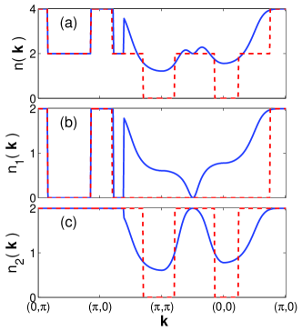
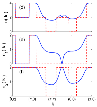
Figure 12: (Color online) (a) Total occupation number $n({\bf k})$ for the two-orbital model Eq. (3) with pairing interaction $V=3$ (continuous lines) and $V=0$ (dashed lines). Parameters: $t_{1}=1.3$, $t_{2}=-1$, $t_{3}=t_{4}=-0.85$, $\mu=1.54$. (b) Same as (a) but for band 1. (c) Same as (b) but for band 2. (d) Total occupation number $n({\bf k})$ for the two-orbital model Eq. (3) with pairing interaction $V=6$ (continuous lines) and $V=0$ (dashed lines). (e) Same as (d) but for band 1. (f) Same as (e) but for band 2.

It is interesting to notice that while $k^{\prime}_{Fh}>k_{Fh}$, on the other hand $k^{\prime}_{Fe}\approx k_{Fe}$ indicating that the reconstruction around the hole pockets is much larger than around the electron pockets. This can also be observed in Fig. 12(b), where we observe unpaired electrons along $X-M$, but not along $\Gamma-X$. The effect occurs in part due to the smaller value of $f({\bf k})$ at the electron pockets but also because, due to the band dispersions, the price in kinetic energy for interband pairing is much larger at the electron pockets than at the hole pockets. The spectral density in Fig. 13 further illustrates that the pairing interaction is more effective along $\Gamma-X$ than along $X-M$. Only shadow spectral weight crosses the chemical potential along $\Gamma-X$, while strong spectral weight crosses the chemical potential twice along $X-M$ and leads to two nodes.

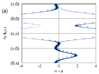
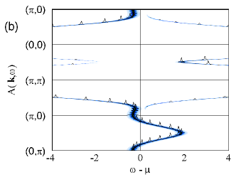
Figure 13: (Color online) (a)Spectral density for the two-orbital model Eq. (3) for a pairing strength $V=3$. The rest of the parameters are as in Fig. 9; (b) same as (a) but for strong pairing $V=6$.

IV.3.3 Strong attractive coupling

Finally, let us consider a much stronger value of the pairing, such as $V=6$, in the BCS region of Fig. 1, for which the only nodes observed are those along $X-Y$, due to the vanishing of the pairing operator. Figures 12(d-f), show that $n({\bf k})$ is discontinuous only along $X-Y$, while it is smooth along all the other directions indicating pairing. Note that $n_{1}({\bf k})=n_{2}({\bf k})$ along $\Gamma-X$ and $X-M$ where interband pairing occurs, while along $\Gamma-M$, $n_{i}({\bf k})$ is smooth but different for each band because the pairing is intraband. The behavior of the spectral functions displayed in Fig. 13 shows that spectral weight only crosses the chemical potential along the $X-Y$ direction. In this situation, in the folded BZ, nodes should occur only at the points where the two electron pockets cross with each other, as indicated in Ref. moreo, . In the rest of the BZ an anisotropic gap will be observed.

IV.4 Stability of the $B_{2g}$ pairing state

Finally, let us discuss the important issue of the stability of the $B_{2g}$ pairing state. It will be assumed, following the notation in Appendix A of Ref. moreo, , that Eq. (3) has arisen from an interorbital attractive potential of the form

$$V_{\bf k,k^{\prime}}=V^{*}(\cos k_{x}+\cos k_{y})(\cos k^{\prime}_{x}+\cos k^{\prime}_{y}),$$ (21)

and that

$$\Delta^{\dagger}({\bf k})=\Delta({\bf k})=V^{*}\Delta(\cos k_{x}+\cos k_{y}),$$ (22)

where

$$\Delta({\bf k}) = -\sum_{{\bf k^{\prime}}}V_{\bf k,k^{\prime}}\langle b_{{\bf k^{\prime}}}\rangle,$$

$$\Delta^{\dagger}({\bf k}) = -\sum_{{\bf k^{\prime}}}V_{\bf k,k^{\prime}}\langle b^{\dagger}_{{\bf k^{\prime}}}\rangle.$$ (23)

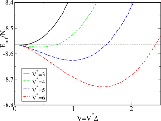
Figure 14: (Color online) Mean field energy per unit site for the interorbital pairing with symmetry $B_{2g}$ for different values of the attraction $V^{*}$ as a function of $V=V^{*}\Delta$.

$V$ in Eq. (5) is then given by $V=V^{*}\Delta$ and the mean-field energy $E_{\rm MF}$ can be calculated for a given $V^{*}$ as a function of $V$. The results are presented in Fig. 14. In this figure, a minimum for $V\neq 0$ can be seen for $V^{*}\geq 3$. This indicates that if the pairing attraction overcomes a finite threshold level, the mean field results presented here with $V\geq 0.2$ will be stable. Thus, if the attraction exists, both multinodal (breached) and states with nodes only along X-Y (strong coupling) are possible.

V Conclusions

Summarizing, in this manuscript the possibility of intra and interband pairing in multiorbital systems has been discussed. While interband pairing has previously been studied in the context of QCD, cold atoms,PhysRevLett.90.047002 ; PhysRevLett.91.032001 heavy fermions,khomskii cuprateskheli , and BCS superconductivity,kumar most of the pairing operators proposed for the pnictides are based on the premise that the pairing has to be purely intraband, i.e., both electrons in the Cooper pairs belonging to the same band, compatible with the assumption that in these superconductors all the action must occur at the Fermi surfaces. However, symmetry considerations show that in models for the pnictides interorbital pairing is allowed with the two members of the Cooper pair belonging to different bands.wan This is not surprising since the bands that determine the electron and hole Fermi surfaces consist of hybridized orbitals. These interorbital pairing operators give rise to not only intra but also interband pairing when the band representation is used. In addition, numerical calculations in a minimal two orbital model for the pnictides favor one of these non-trivial pairing operators.ours ; moreo As a consequence, a clear discussion of the role of interband pairing is necessary.

The explicit calculations shown here of the electronic occupation in the orbital and the band representations, as well as the calculation of the spectral functions showing the distribution of Bogoliubov bands, may offer guidance in the interpretation of ARPES experiments. In particular, most ARPES measurements determine the FS in the normal state and study the opening of the superconducting gap by monitoring $A(k_{F},\omega)$ as they lower the temperature.arpes ; arpes2 ; arpes22 ; arpes3 ; hsieh Notice that this approach would miss the nodes associated with the “breached” phase since in the superconducting state a gap would be observed in $A(k_{F},\omega)$ while the node would be detected in $A(k^{\prime}_{F},\omega)$. Thus, experimentalists should investigate the possibility of nodes at points in momentum space that do not belong to the normal state FS and they must keep in mind that some of the nodes may be determined by shadow bands with very small spectral weight.

The most recent experimental results with the polarization dependence of the ARPES spectra for BaFe_1.85Co_0.15As₂ provided the allowed contribution of each of the five $3d$ orbitals to the electron and hole Fermi surfaces.FeAs_orb_FS While discrepancies with proposed four and five orbital models are remarked in that publication, it is interesting to observe that the minimal two-orbital model addressed here does not contradict the ARPES findings if we disregard the additional $\beta$ hole pocket FS that they present, which is reasonable because it has $d_{x^{2}-y^{2}}$ character, an orbital not included in the minimal model considered here. In fact, along their $\Gamma-M$ direction, which corresponds to our $\Gamma-X$, our first hole FS is purely $d_{xz}$ as it is their $\alpha_{\pi}$ hole FS; our second hole FS, which arises upon folding our extended FS along $X-Y$ is purely $d_{yz}$, as it is their $\alpha_{\sigma}$ hole FS, and our electron FS is purely $d_{yz}$ as it is their $\gamma$ electron FS. Our second electron FS (obtained upon folding) has a purely $d_{xz}$ character, while their electron FS $\gamma^{\prime}/\alpha^{\prime}$ appears to be mostly $d_{yz}$ and $d_{xy}$, but with some amounts of $d_{xz}$ as well. Along the diagonal direction $\Gamma-X$, which corresponds to our $\Gamma-M$, the two hole Fermi surfaces are a symmetric admixture of $d_{xz}$ and $d_{yz}$, exactly as in the two-orbital model.hoppings Thus, these similarities between the experimental results and the band composition of the simple two-orbital model offer encouragement towards exploring whether the main physics of the pnictides can be captured with such a minimum number of degrees of freedom.

We have also mentioned in the text that the symmetry of the lattice and of the orbitals introduce constraints on the possible pairing operators. In general, a purely intraband pairing, such as the proposed $s_{\pm}$ state,kuroki ; Mazin:2008p1695 ; korshunov ; parker would occur only if the coupling of the electrons with the source of the attraction is identical for all orbitals. Considering the different spatial orientations of the orbitals, it is not obvious that this should be the case, since, as discussed in the Introduction, phonons couple differently to electrons in the $p_{z}$ and $p_{x}$ boron orbitals in the case of MgB₂. Thus, if indeed the coupling results to be the same for all $3d$ orbitals we could use this fact to elucidate the pairing mechanism; but, if this is not the case, we would expect some degree of interband pairing, at least in some regions of the Brillouin zone and, thus, it is important to study the experimental and theoretical consequences of such a possibility.

- (1) Y. Kamihara, T. Watanabe, M. Hirano, and H. Hosono, J. Am. Chem. Soc. 130, 3296 (2008).
- (2) G. F. Chen, Z. Li, G. Li, J. Zhou, D. Wu, J. Dong, W. Z. Hu, P. Zheng, Z. J. Chen, H. Q. Yuan, J. Singleton, J. L. Luo, and N. L. Wang, Phys. Rev. Lett. 101, 057007 (2008).
- (3) G. F. Chen, Z. Li, D. Wu, G. Li, W. Z. Hu, J. Dong, P. Zheng, J. L. Luo, and N. L. Wang, Phys. Rev. Lett. 100, 247002 (2008).
- (4) H.-H. Wen, G. Mu, L. Fang, H. Yang, and X. Zhu, Europhys. Lett. 82, 17009 (2008).
- (5) X. H. Chen, T. Wu, G. Wu, R. H. Liu, H. Chen, and D. F. Fang, Nature 453, 761 (2008).
- (6) Z. A. Ren, J. Yang, W. Lu, W. Yi, G. Che, X. Dong, L. Sun, and Z. Zhao, Mater. Res. Innovat. 12, 105 (2008).
- (7) Z. A. Ren, W. Lu, J. Yang, W. Yi, X.-L. Shen, Z.-C. Li, G.-C. Che, X.-L. Dong, L.-L. Sun, F. Zhou, and Z.-X. Zhao, Chin. Phys. Lett. 25, 2215 (2008).
- (8) Z.-A. Ren, G.-C. Che, X.-L. Dong, J. Yang, W. Lu, W. Yi, X.-L. Shen, Z.-C. Li, L.-L. Sun, F. Zhou, and Z.-X. Zhao, Europhys. Lett. 83, 17002 (2008).
- (9) S. Lebegue, Phys. Rev. B 75, 035110 (2007).
- (10) D. J. Singh and M.-H. Du, Phys. Rev. Lett. 100, 237003 (2008).
- (11) G. Xu, W. Ming, Y. Yao, X. Dai, S.-C. Zhang, and Z. Fang, Europhys. Lett. 82, 67002 (2008).
- (12) C. Cao, P. J. Hirschfeld, and H.-P. Cheng, Phys. Rev. B 77, 220506 (2008).
- (13) H.-J. Zhang, G. Xu, X. Dai, and Z. Fang, Chin. Phys. Lett. 26, 017401 (2009).
- (14) P. A. Lee and X.-G. Wen, Phys. Rev. B 78, 144517 (2008).
- (15) H. Suhl, B. T. Matthias, and L. R. Walker, Phys. Rev. Lett. 3, 552 (1959).
- (16) J. Bardeen, L. N. Cooper, and J. R. Schrieffer, Phys. Rev. 108, 1175 (1957).
- (17) J. Nagamatsu, N. Nakagawa, T. Muranaka, Y. Zenitani, and J. Akimitsu, Nature 410, 63 (2001).
- (18) H. J. Choi, D. Roundy, H. Sun, M. L. Cohen, and S. G. Louie, Nature 418, 758 (2002).
- (19) Y. Wang, T. Plackowski, and A. Junod, Physica C 355, 179 (2001).
- (20) F. Bouquet, R. A. Fisher, N. E. Phillips, D. G. Hinks, and J. D. Jorgensen, Phys. Rev. Lett. 87, 047001 (2001).
- (21) H. D. Yang, J.-Y. Lin, H. H. Li, F. H. Hsu, C. J. Liu, S.-C. Li, R.-C. Yu, and C.-Q. Jin, Phys. Rev. Lett. 87, 167003 (2001).
- (22) P. Szabó, P. Samuely, J. Kačmarčík, T. Klein, J. Marcus, D. Fruchart, S. Miraglia, C. Marcenat, and A. G. M. Jansen, Phys. Rev. Lett. 87, 137005 (2001).
- (23) F. Giubileo, D. Roditchev, W. Sacks, R. Lamy, D. X. Thanh, J. Klein, S. Miraglia, D. Fruchart, J. Marcus, and P. Monod, Phys. Rev. Lett. 87, 177008 (2001).
- (24) X. K. Chen, M. J. Konstantinović, J. C. Irwin, D. D. Lawrie, and J. P. Franck, Phys. Rev. Lett. 87, 157002 (2001).
- (25) S. Tsuda, T. Yokoya, T. Kiss, Y. Takano, K. Togano, H. Kito, H. Ihara, and S. Shin, Phys. Rev. Lett. 87, 177006 (2001).
- (26) K. Kuroki, S. Onari, R. Arita, H. Usui, Y. Tanaka, H. Kontani, and H. Aoki, Phys. Rev. Lett. 101, 087004 (2008).
- (27) I. Mazin, D. Singh, M. Johannes, and M. Du, Phys. Rev. Lett. 101, 057003 (2008).
- (28) X. Dai, Z. Fang, Y. Zhou, and F.-C. Zhang, Phys. Rev. Lett. 101, 057008 (2008).
- (29) Q. Han, Y. Chen, and Z. D. Wang, Europhys. Lett. 82, 37007 (2008).
- (30) M. M. Korshunov and I. Eremin, Phys. Rev. B 78, 140509 (2008).
- (31) G. Baskaran, arXiv:0804.1341, 2008.
- (32) T. Yildirim, Phys. Rev. Lett. 101, 057010 (2008).
- (33) Q. Si and E. Abrahams, Phys. Rev. Lett. 101, 076401 (2008).
- (34) Z.-J. Yao, J.-X. Li, and Z. D. Wang, New J. Phys. 11, 025009 (2009).
- (35) C. Xu, M. Müller, and S. Sachdev, Phys. Rev. B 78, 020501 (2008).
- (36) E. Manousakis, J. Ren, S. Meng, and E. Kaxiras, Phys. Rev. B 78, 205112 (2008).
- (37) O. Dolgov, I. Mazin and D. Parker, Phys. Rev. B 79, 060502(R)(2009).
- (38) M. Daghofer, A. Moreo, J. A. Riera, E. Arrigoni, D. J. Scalapino, and E. Dagotto, Phys. Rev. Lett. 101, 237004 (2008).
- (39) S. Raghu, X.-L. Qi, C.-X. Liu, D. J. Scalapino, and S.-C. Zhang, Phys. Rev. B 77, 220503 (2008).
- (40) A. Moreo, M. Daghofer, J. A. Riera, and E. Dagotto, Phys. Rev. B 79, 134502 (2009).
- (41) W. V. Liu and F. Wilczek, Phys. Rev. Lett. 90, 047002 (2003).
- (42) E. Gubankova, W. V. Liu, and F. Wilczek, Phys. Rev. Lett. 91, 032001 (2003).
- (43) O. Dolgov, E. Fetisov, D. Khomskii, and K. Svozil, Z. Phys. B 67, 63 (1987).
- (44) J. Tahir-Kheli, Phys. Rev. B 58, 12307 (1998).
- (45) N. Kumar and K. P. Sinha, Phys. Rev. 174, 482 (1968).
- (46) It is interesting to observe that in the undoped limit there are also three regimes: normal, coexisting magnetism and metallicity, and magnetism without a Fermi surface. For details see R. Yu, K. T. Trinh, A. Moreo, M. Daghofer, J. A. Riera, S. Haas, and E. Dagotto, Phys. Rev. B 79, 104510 (2009).
- (47) Z.-H. Wang, H. Tang, Z. Fang, and X. Dai, arXiv:0805.0736, 2008.
- (48) J. Shi, arXiv:0806.0259, 2008.
- (49) W.-L. You, S.-J. Gu, G.-S. Tian, and H.-Q. Lin, Phys. Rev. B 79, 014508 (2009)
- (50) Y. Wan and Q.-H. Wang, Europhys. Lett. 85, 57007 (2009).
- (51) Y. Zhou, W-Q. Chen, and F-C. Zhang, Phys. Rev. B 78, 064514 (2008).
- (52) P. Goswami, P. Nikolic, and Q. Si, arZiv:0905.2634, 2009.
- (53) D. Parker, O. V. Dolgov, M. M. Korshunov, A. A. Golubov, and I. I. Mazin, Phys. Rev. B 78, 134524 (2008).
- (54) T. Kondo, A. F. Santander-Syro, O. Copie, C. Liu, M. E. Tillman, E. D. Mun, J. Schmalian, S. L. Bud’ko, M. A. Tanatar, P. C. Canfield, and A. Kaminski, Phys. Rev. Lett. 101, 147003 (2008).
- (55) H. Ding, P. Richard, K. Nakayama, K. Sugawara, T. Arakane, Y. Sekiba, A. Takayama, S. Souma, T. Sato, T. Takahashi, Z. Wang, X. Dai, Z. Fang, G. F. Chen, J. L. Luo, and N. L. Wang, EPL 83, 47001 (2008).
- (56) L. Wray, D. Qian, D. Hsieh, Y. Xia, L. Li, J.G. Checkelsky, A. Pasupathy, K.K. Gomes, C. V. Parker, A.V. Fedorov, G.F. Chen, J.L. Luo, A. Yazdani, N.P. Ong, N.L. Wang, M.Z. Hasan, Phys. Rev. B 78, 184508 (2008).
- (57) V. B. Zabolotnyy, D. S. Inosov, D. V. Evtushinsky, A. Koitzsch, A. A. Kordyuk, J. T. Park, D. Haug, V. Hinkov, A. V. Boris, D. L. Sun, G. L. Sun, C. T. Lin, B. Keimer, M. Knupfer, B. Buechner, A. Varykhalov, R. Follath, and S. V. Borisenko, Nature 457, 569 (2009).
- (58) D. Hsieh, Y. Xia, L. Wray, D. Qian, K. Gomes, A. Yazdani, G.F. Chen, J.L. Luo, N.L. Wang, and M.Z.Hasan, arXiv:0812.2289 (2008).
- (59) Y. Zhang, B. Zhou, F. Chen, J. Wei, M. Xu, L. X. Yang, C. Fang, W. F. Tsai, G. H. Cao, Z. A. Xu, M. Arita, C. Hong, K. Shimada, H. Namatame, M. Taniguchi, J. P. Hu, and D. L. Feng, arXiv:0904.4022, 2009.
- (60) Notice that we have exchanged the values of and provided in Ref. scalapino, in order to reproduce the ARPES orbital composition.