Production of $Z^{0}$ bosons with rapidity gaps:
exclusive photoproduction in $\gamma p$ and $pp$ collisions
and inclusive double diffractive $Z^{0}$’s

Abstract

We extend the $k_{\perp}$–factorization formalism for exclusive photoproduction of vector mesons to the production of electroweak $Z^{0}$ bosons. Predictions for the $\gamma p\to Z^{0}p$ and $pp\to ppZ^{0}$ reactions are given using an unintegrated gluon distribution tested against deep inelastic data. We present distributions in the $Z^{0}$ rapidity, transverse momentum of $Z^{0}$ as well as in relative azimuthal angle between outgoing protons. The contributions of different flavours are discussed. Absorption effects lower the cross section by a factor of 1.5-2, depending on the Z-boson rapidity. We also discuss the production of $Z^{0}$ bosons in central inclusive production. Here rapidity and $(x_{{\bf I\!P},1},x_{{\bf I\!P},2})$ distributions of $Z^{0}$ are calculated. The corresponding cross section is about three orders of magnitude larger than that for the purely exclusive process.

I Introduction

There has been recently much experimental progress in the field of central exclusive production. The observation of exclusive central dijets exclusive_dijets , as well as charmonia/$\mu^{+}\mu^{-}$–pairsexclusive_charmonia has clearly demonstrated the feasibilty of detecting exclusive final states at collider energies. These are good prospects for possible future studies at the LHC, addressing a wide range of physics problems, from Higgs physics, to the investigations of the QCD–Pomeron and hadronic structure of the produced particles. For recent reviews see for example Martin_epiphany for theory/phenomenology, and experiment for experiment.

The mechanism of the reaction strongly depends on the centrally produced particle, in particular its spin, parity, C-parity and internal stucture. For heavy vector quarkonia such as $J/\Psi$ and $\Upsilon$ the photon-pomeron fusion is the dominant mechanism (for recent calculations see e.g. SS07 ; RSS08 ). The same is expected for the $Z^{0}$ gauge boson GM08 ; MW08 . The dominant reaction mechanism is shown in Fig.1.

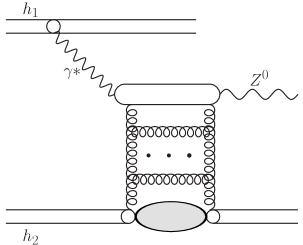
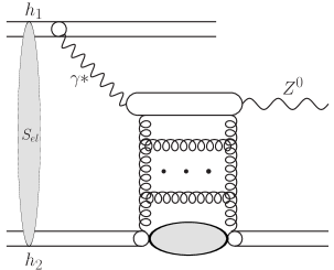
Figure 1: Diagrammatic representation of the photon–Pomeron fusion mechanism of exclusive $Z^{0}$–boson production in hadronic collisions.

Here, the essential ingredient is the $\gamma p\to Z^{0}p$ subprocess, which proceeds through the $q\bar{q}$ component of the virtual photon. There is a strong similarity to the production of $q\bar{q}$ vector mesons, and one would expect the QCD description of this process to follow from the color dipole/$k_{\perp}$-factorization approach to vector meson production (for a review, see INS06 ) by straightforward modifications GM08 ; MW08 . The important distinction to the case of vector meson production is the fact that the $q\bar{q}$ pair coupling to the $Z^{0}$–boson can be put on its mass-shell. In the impact parameter space color-dipole formulation, this requires to continue the light–cone wavefunction of the $Z^{0}$ to the region of complex arguments. The resulting highly oscillatory integrands are however not straightforward to handle MW08 .

In the momentum space representation given in this work, the situation is more transparent, and the numerics poses no special problems.

Previous calculations of the $pp\to ppZ^{0}$ process made use of the equivalent-photon approximation (EPA) and did not include absorption effects. In the EPA only total cross section or rapidity distribution of the $Z^{0}$ boson can be calculated. In this paper we use the formalism of SS07 ; RSS08 to perform the calculation at the amplitude–level, which allows us to calculate other differential observables (e.g. in $Z^{0}$ boson transverse momentum or correlation in relative azimuthal angle between outgoing protons) and to include absorption corrections.

The cross sections for exclusive $Z^{0}$ production for both the Tevatron and LHC are very small. In fact a recent search for exclusive $Z^{0}$CDF_Z0_exclusive only puts rather generous bounds on the cross section. The exclusive events are characterized by large rapidity gaps between centrally produced $Z^{0}$ bosons and very forward or very backward final state nucleons. Another process with these features is the inclusive double-diffractive production of $Z^{0}$, which to our knowledge was not previously calculated the literature . In the latter case the $Z^{0}$ in the central rapidity region is associated with low-multiplicity hadronic activity.

II $\gamma p\to Z^{0}p$ photoproduction process

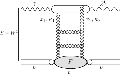
Figure 2: A pQCD diagram for the $\gamma p\to Z^{0}p$ amplitude at large $\gamma p$ cm-energy. The gluon exchange ladder is modelled by the unintegrated gluon distribution of the target.

Before we go to the hadronic reaction let us start from the real photoproduction process depicted in Fig.2. The forward production amplitude can be written very much the same way as for exclusive photoproduction of vector quarkonia (see for example INS06 ):

$${\cal M}(W,\Delta^{2}=0)=W^{2}\,\ \sum_{f}{4\pi\alpha g_{V}^{f}\over 4\pi^{2}}\,2\int_{0}^{1}dz\int d^{2}\mbox{\boldmath$k$}{{\cal{A}}_{f}(z,\mbox{\boldmath$k$}^{2})\over\mbox{\boldmath$k$}^{2}+m_{f}^{2}-z(1-z)M_{Z}^{2}-i\epsilon}\;.$$ (1)

As was already shown in GM08 ; MW08 , only the vectorial part of the $Z^{0}q\bar{q}$–coupling contributes to the forward amplitude,

$$g_{V}^{f}={I_{3f}-2e_{f}\sin^{2}\Theta_{W}\over\sin 2\Theta_{W}}$$ (2)

is the relevant weak vector coupling, $I_{3f}$ is the weak isospin of a quark of flavour $f$, $e_{f}$ is its charge, and $\Theta_{W}$ is the Weinberg angle. The imaginary part of ${\cal{A}}_{f}$ can be obtained from the results given for vector meson production with the $\gamma_{\mu}$ vertex in INS06 . Performing azimuthal integrals one obtains RSS08 :

$$\Im m{\cal A}_{f}(z,\mbox{\boldmath$k$}^{2})=\pi\int_{0}^{\infty}{\pi d\kappa^{2}\over\kappa^{4}}\alpha_{S}(q^{2}){\cal{F}}(x,\kappa^{2})(A_{0f}(z,k^{2})\;W_{0f}(k^{2},\kappa^{2})+A_{1f}(z,k^{2})\;W_{1f}(k^{2},\kappa^{2}))$$ (3)

with

$$A_{0f}(z,k^{2})=m_{f}^{2}\,\,,\,\,A_{1f}(z,k^{2})=[z^{2}+(1-z)^{2}]\frac{k^{2}}{k^{2}+m_{f}^{2}}\,,$$

and

$$W_{0f}(k^{2},\kappa^{2}) = {1\over k^{2}+m_{f}^{2}}-{1\over\sqrt{(k^{2}-m_{f}^{2}-\kappa^{2})^{2}+4m_{f}^{2}k^{2}}}\;,$$

$$W_{1f}(k^{2},\kappa^{2}) = 1-{k^{2}+m_{f}^{2}\over 2k^{2}}\left(1+{k^{2}-m_{f}^{2}-\kappa^{2}\over\sqrt{(k^{2}-m_{f}^{2}-\kappa^{2})^{2}+4m_{f}^{2}k^{2}}}\,\right)\;.$$

The strong coupling $\alpha_{s}$ enters at the scale $q^{2}=\max\{\mbox{\boldmath$k$}^{2}+m_{f}^{2},\mbox{\boldmath$\kappa$}^{2}\}$. The unintegrated gluon distribution ${\cal{F}}(x,\mbox{\boldmath$\kappa$}^{2})$ is sampled at $x=c_{skewed}\cdot M_{Z}^{2}/W^{2}$ with $c_{skewed}=0.41$. This shifted value of $x$ simulates the prescription of Shuvaev to obtain the skewed distribution from the diagonal one, and is valid for the particular gluon distribution we use INS06 . Now, let

$$z_{\pm}={1\over 2}\left(1\pm\sqrt{1-{4m_{f}^{2}\over M_{Z}^{2}}}\right)\,,$$ (4)

then, the integration domain $z\in[0,1]$ must be split into $[0,z_{-}]\cup[z_{-},z_{+}]\cup[z_{+},1]$. Apparently, within the subdomain $[z_{-},z_{+}]$ the denominator in Eq.(1) can go to zero, which means that the $q\bar{q}$ state after the interaction can go on-shell. This leads to a rotation of the complex phase of the dominantly imaginary amplitude. For $z\in[z_{-},z_{+}]$, one must use the Plemelj-Sokhocki formula

$${1\over\mbox{\boldmath$k$}^{2}+m_{f}^{2}-z(1-z)M_{Z}^{2}-i\epsilon}=\mathrm{PV}{1\over\mbox{\boldmath$k$}^{2}+m_{f}^{2}-z(1-z)M_{Z}^{2}}+\,i\,\pi\,\delta(\mbox{\boldmath$k$}^{2}+m_{f}^{2}-z(1-z)M_{Z}^{2})\,,$$

where PV denotes the principal value integral. It can be evaluated as

$$\mathrm{PV}\,\int_{0}^{\infty}d\mbox{\boldmath$k$}^{2}{{\cal A}_{f}(z,\mbox{\boldmath$k$}^{2})\over\mbox{\boldmath$k$}^{2}-\tau^{2}} = \int_{0}^{(1+\lambda)\tau^{2}}d\mbox{\boldmath$k$}^{2}{{\cal A}_{f}(z,\mbox{\boldmath$k$}^{2})-{\cal A}_{f}(z,\tau^{2})\over\mbox{\boldmath$k$}^{2}-\tau^{2}}+\int_{(1+\lambda)\tau^{2}}^{\infty}d\mbox{\boldmath$k$}^{2}{{\cal A}_{f}(z,\mbox{\boldmath$k$}^{2})\over\mbox{\boldmath$k$}^{2}-\tau^{2}}$$

$$+ {\cal A}_{f}(z,\tau^{2})\,\log(\lambda)\,,$$

for an arbitrary positive value of $\lambda$. Here $\tau^{2}=z(1-z)M_{Z}^{2}-m_{f}^{2}$ is positive in the relevant integration domain.

Another distinction in comparison to the vector-meson(VM) photoproduction is worth a comment. Effectively, we replace the non–perturbative light cone wave–function of the VM by the propagator:

$$\psi_{V}(z,\mbox{\boldmath$k$}^{2})\to{1\over\mbox{\boldmath$k$}^{2}+m_{f}^{2}-z(1-z)M_{Z}^{2}-i\epsilon}\,.$$ (7)

While in the case of vector–mesons, the light–cone wave–function will suppress the endpoint–region $z,1-z\ll 1$, no such suppression of asymmetric $q\bar{q}$ pairs is available here. Incidentally, in impact parameter space asymmetric pairs correspond to large dipole sizes NZ91 , and it is precisely the wave–function suppresion of large dipoles, which leads to the dipole–size scanning property KNNZ93 ; INS06 of VM production amplitudes. Therefore, strictly speaking, the $Z^{0}$ production cross section is not purely perturbatively calculable, but one must rely on the ability of the color–dipole/$k_{\perp}$-factorization approaches to properly factorize the large dipole/infrared contributions. Compare this to the scaling contribution of large dipoles to the transverse DIS structure function $F_{T}(x,Q^{2})=2xF_{1}(x,Q^{2})$ NZ91 ; IN_glue at large $Q^{2}$.

Finally, we note, that we restore the real part of the amplitude by substituting

$${\cal{A}}_{f}=(i+\rho)\Im m{\cal{A}}_{f}\,,$$ (8)

where $\rho=\tan(\pi\Delta_{\bf I\!P}/2)$, and $\Delta_{\bf I\!P}=\partial\log\Im m{\cal{A}}_{f}/\partial\log W^{2}$, and the $\gamma p\to Z^{0}p$ amplitude within the diffraction cone is given by

$${\cal{M}}(W^{2},\Delta^{2})={\cal{M}}(W^{2},\Delta^{2}=0)\,\exp[Bt]\,,$$ (9)

where $t=-\Delta^{2}$ and the running diffraction slope is taken as

$$B=B_{0}+2\alpha_{eff}^{\prime}\log\Big{(}W^{2}/W_{0}^{2}\Big{)}\,,$$ (10)

with $B_{0}=3.5\,\mathrm{GeV}^{-2}$, $\alpha^{\prime}_{eff}=0.164\,\mathrm{GeV}^{-2}$, and $W_{0}=95\,\mathrm{GeV}$ H1_JPsi .

III $pp\to ppZ^{0}$ exclusive hadroproduction

Assuming only helicity conserving processes the Born amplitude for the $pp\to ppZ^{0}$ reaction is a sum of amplitudes of the processes shown in Fig.1 and can be written through the amplitudes of photoproduction processes $\gamma h_{2}\to Z^{0}h_{2}$ or $\gamma h_{2}\to Z^{0}h_{2}$, discussed above, in the form of the vector

$${\mbox{\boldmath$M$}}^{(0)}_{h_{1}h_{2}\to h_{1}h_{2}Z^{0}}(\mbox{\boldmath$p$}_{1},\mbox{\boldmath$p$}_{2}) = e_{1}\sqrt{4\pi\alpha_{em}}F_{1}(t_{1})\frac{2{\mbox{\boldmath$p$}}_{1}}{z_{1}t_{1}}\cdot{\cal M}_{\gamma^{*}h_{2}\to Z^{0}h_{2}}(Q_{1}^{2};s_{2},t_{2})$$ (11)

$$+ e_{2}\sqrt{4\pi\alpha_{em}}F_{1}(t_{2})\frac{2{\mbox{\boldmath$p$}}_{2}}{z_{2}t_{2}}\cdot{\cal M}_{\gamma^{*}h_{1}\to Z^{0}h_{1}}(Q_{2}^{2};s_{1},t_{1})\;.$$

Above $Q_{1}^{2}=-t_{1}$ and $Q_{2}^{2}=-t_{2}$ are virtualities of photons, $F_{1}$ is the familiar Dirac electromagnetic form factor of the proton/antiproton and $\mbox{\boldmath$p$}_{1}$, $\mbox{\boldmath$p$}_{2}$ are transverse momenta of outgoing protons. In the present analysis we shall use a simple parametrization of the Dirac electromagnetic form factor $F_{1}$ taken from Ref.DDLN02 .

The dependence of the the virtual photoproduction subprocess amplitude on space-like virtuality of the photon $Q^{2}$ is in practice entirely negligible (recall that $Q^{2}\ll M_{Z}^{2}$).

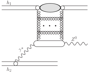
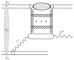
Figure 3: Diagrammatic representation of the exclusive $Z^{0}$ production amplitude with inclusion of absorptive corrections. The absorptive corrections are calculable in terms of the hadron–hadron elastic $S$-matrix.

In the hadroproduction process one has to include additional absorption corrections. The relevant formalism for the calculation of amplitudes and cross–sections was reviewed in some detail in Ref.SS07 . Here we give only a the main formulas. The basic mechanisms are shown in Fig.6.

Inclusion of absorptive corrections (the ’elastic rescattering’) leads in momentum space to the full, absorbed amplitude

$$\mbox{\boldmath$M$}(\mbox{\boldmath$p$}_{1},\mbox{\boldmath$p$}_{2}) =\int{d^{2}\mbox{\boldmath$k$}\over(2\pi)^{2}}\,S_{el}(\mbox{\boldmath$k$})\,\mbox{\boldmath$M$}^{(0)}(\mbox{\boldmath$p$}_{1}-\mbox{\boldmath$k$},\mbox{\boldmath$p$}_{2}+\mbox{\boldmath$k$})=\mbox{\boldmath$M$}^{(0)}(\mbox{\boldmath$p$}_{1},\mbox{\boldmath$p$}_{2})-\delta\mbox{\boldmath$M$}(\mbox{\boldmath$p$}_{1},\mbox{\boldmath$p$}_{2})\,.$$

With

$$S_{el}(\mbox{\boldmath$k$})=(2\pi)^{2}\delta^{(2)}(\mbox{\boldmath$k$})-{1\over 2}T(\mbox{\boldmath$k$})\,\,\,,\,\,\,T(\mbox{\boldmath$k$})=\sigma^{p\bar{p}}_{tot}(s)\,\exp\Big{(}-{1\over 2}B_{el}\mbox{\boldmath$k$}^{2}\Big{)}\,,$$ (13)

where at Tevatron energy $\sqrt{s}$ = 1800 GeV $\sigma^{p\bar{p}}_{tot}(s)=76$ mb, $B_{el}=17$ GeV^-2 CDF_total , the absorptive correction $\delta\mbox{\boldmath$M$}$ reads

$$\delta\mbox{\boldmath$M$}(\mbox{\boldmath$p$}_{1},\mbox{\boldmath$p$}_{2})=\int{d^{2}\mbox{\boldmath$k$}\over 2(2\pi)^{2}}\,T(\mbox{\boldmath$k$})\,\mbox{\boldmath$M$}^{(0)}(\mbox{\boldmath$p$}_{1}-\mbox{\boldmath$k$},\mbox{\boldmath$p$}_{2}+\mbox{\boldmath$k$})\,.$$ (14)

The differential cross section is given in terms of $M$ as

$$d\sigma={1\over 512\pi^{4}s^{2}}|\mbox{\boldmath$M$}|^{2}\,dydt_{1}dt_{2}d\phi\,,$$ (15)

where $y$ is the rapidity of the $Z^{0}$-boson, $t_{1}$, $t_{2}$ are four-momentum transfers squared, and $\phi$ is the angle between transverse momenta $\mbox{\boldmath$p$}_{1}$ and $\mbox{\boldmath$p$}_{2}$.

IV Inclusive double diffactive production of $Z^{0}$

The purely exclusive process discussed so far can be characterized by large rapidity gaps between the centrally produced $Z^{0}$ and forward/backward emitted protons/antiprotons. Can the rapidity gap method be used to identify this process? The discussed exclusive process is not the only one with double rapidity gaps. The inclusive double-pomeron cross section for $Z^{0}$ boson production was apparently not previously calculated. The mechanism is depicted in Fig.4.

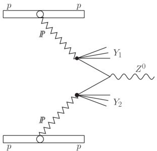
Figure 4: Pomeron–Pomeron fusion representation of the central diffractive inclusive $Z^{0}$ production. The hard subprocess is viewed as a collision of partons of the Pomeron.

Following Ingelman and Schlein Ingelman_Schlein , one may try to estimate the hard diffractive process by assuming that the Pomeron has a well defined partonic structure, and that the hard process takes place in a Pomeron–Pomeron collision. Then the rapidity distribution of $Z^{0}$–bosons would be obtained from

$${d\sigma(pp\to ppZ^{0}X)\over dy}=K\,\sum_{f}\sigma(q_{f}\bar{q}_{f}\to Z^{0};x_{1}x_{2}s)\,\Big{(}x_{1}q_{f}^{D}(x_{1},\mu^{2})\,x_{2}\bar{q}_{f}^{D}(x_{2},\mu^{2})+(1\leftrightarrow 2)\Big{)}\,.$$

(16)

Here

$$x_{1}={M_{Z}\over\sqrt{s}}e^{y},\,\,\,x_{2}={M_{Z}\over\sqrt{s}}e^{-y},$$

$\sigma_{q_{f}{\bar{q}}_{f}\to Z^{0}}({\hat{s}})$ is the elementary “zeroth-order” flavour-dependent cross sections (see e.g. BP87 ). $K$ in Eq.(16) stands for the Drell-Yan type $K$-factor which includes approximately pQCD NLO corrections BP87 .

The effective ’diffractive’ quark distribution of flavour $f$ is given by a convolution of the flux of Pomerons $f_{\bf I\!P}(x_{\bf I\!P})$ and the parton distribution in a Pomeron $q_{f/{\bf I\!P}}(\beta,\mu^{2})$:

$$q_{f}^{D}(x_{1},\mu^{2})=\int dx_{\bf I\!P}d\beta\,\delta(x-x_{\bf I\!P}\beta)q_{f/{\bf I\!P}}(\beta,\mu^{2})\,f_{\bf I\!P}(x_{\bf I\!P})\,=\int_{x}^{1}{dx_{\bf I\!P}\over x_{\bf I\!P}}\,f_{\bf I\!P}(x_{\bf I\!P})q_{f/{\bf I\!P}}({x\over x_{\bf I\!P}},\mu^{2})\,.$$

The flux of Pomerons $f_{\bf I\!P}(x_{\bf I\!P})$ enters in the form integrated over four–momentum transfer

$$f_{\bf I\!P}(x_{\bf I\!P})=\int_{t_{min}}^{t_{max}}dt\,f(x_{\bf I\!P},t)\,,$$ (18)

with $t_{min},t_{max}$ being the kinematic boundaries.

Both pomeron flux factors $f_{{\bf I\!P}}(x_{{\bf I\!P}},t)$ as well as quark/antiquark distributions in pomeron were taken from the H1 collaboration analysis of diffractive structure function and/or from the analysis of diffractive dijets at HERA H1 . The factorization scale is taken as $\mu_{F}^{2}=M_{Z}^{2}$.

Besides the Pomeron–exchange, one must also include the secondary Reggeon–exchange contribution, which dominates at larger $x_{\bf I\!P}$. Consequently, a number of interference contributions arise, which are shown diagramatically in Fig. 5. As we wish to use the results of the H1 analysis of diffractive DIS at HERA, we have to omit a number of interference terms, which would involve Reggeon–Pomeron interference structure functions that have been neglected in the H1 analysis. Incidentally, within pQCD, there is no reason why interference terms should be small, and in fact, they enter the diffractive structure functions in the maximal possible way WS98 . While one obtains good fits of HERA data, even omitting the ${\bf I\!R}-{\bf I\!P}$ interference, the rather unphysical values of the so-extracted Reggeon trajectory parameters show the limitations of such a procedure. Clearly though, a full reanalysis of H1-data is not warranted for our purpose of obtaining a first estimate of the $Z^{0}$-production cross section.

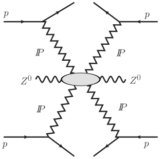
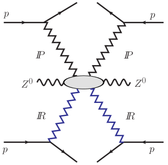
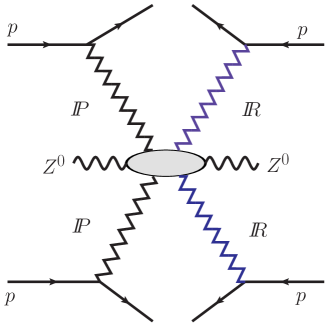
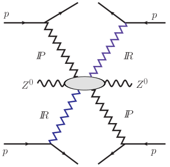
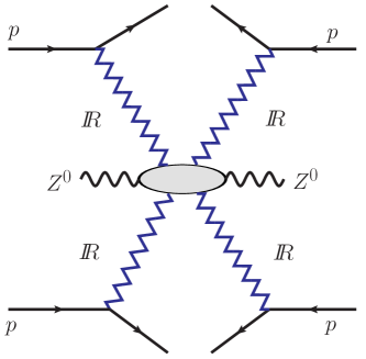
Figure 5: Mueller-Kancheli diagrams for the process $pp\to p+\mathrm{gap}+Z^{0}X+\mathrm{gap}+p$. Interference diagrams of type (c,d), which would involve ${\bf I\!P}-{\bf I\!R}$ interference structure functions are neglected.

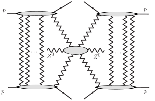
Figure 6: Absorptive correction to the ${\bf I\!P}$–exchange contribution.

It is however obvious, that the naive factorization prescription of Eq.(16) cannot be correct. It neglects rescattering effects of incoming protons shown in Fig.6. Indeed such diagrams quantify the probability that protons emerge intact out of the interactions region in a regime where the typical events are highly inelastic and many channels are open Bjorken . Here we restrict ourselves to only a ’minimal’ scenario of factorization breaking induced by eikonalized multiple scatterings, following the formalism of Ref.TerMartirosyan (for a somewhat modernized version, see KMR_eikonal ).

We do not enter here the debate on the possible relevance of multiple–Pomeron vertices (see for example the reviews Martin_epiphany ; Maor and references therein), but keep in mind that our treatment of absorption may require a revision after better knowledge on soft interactions at the LHC has been acquired.

The relevant formulas are most easily written in impact parameter space. As in practice $t_{i}\sim-\mbox{\boldmath$q$}_{i}^{2}$, where $\mbox{\boldmath$q$}_{i}$ is the transverse momentum transfer to proton $i$, we can write

$$f_{\bf I\!P}(x_{\bf I\!P},t)=f_{\bf I\!P}(x_{\bf I\!P},\mbox{\boldmath$q$})=f_{\bf I\!P}(x_{\bf I\!P})\exp[-B\mbox{\boldmath$q$}^{2}]\,,$$ (19)

where $B=B(x_{\bf I\!P})=B_{D}+2\alpha^{\prime}_{\bf I\!P}\log(1/x_{\bf I\!P})$ is the $x_{\bf I\!P}$–dependent diffractive slope. We follow the $H1$-analysis H1 , and use the central values of their fit $B_{D}=5.5\,\mathrm{GeV}^{-2},\alpha^{\prime}_{\bf I\!P}=0.06\,\mathrm{GeV}^{-2}$ Then, in impact parameter space, we have

$$f_{\bf I\!P}(x_{\bf I\!P},\mbox{\boldmath$b$})=\int{d^{2}\mbox{\boldmath$q$}\over(2\pi)^{2}}\,f_{\bf I\!P}(x_{\bf I\!P},\mbox{\boldmath$q$})\,\exp[-i\mbox{\boldmath$b$}\mbox{\boldmath$q$}]={f_{\bf I\!P}(x_{\bf I\!P})\over 4\pi B}\exp[-{\mbox{\boldmath$b$}^{2}\over 4B}]\equiv f_{\bf I\!P}(x_{\bf I\!P})\,t_{\bf I\!P}(x_{\bf I\!P},\mbox{\boldmath$b$})\,.$$

(20)

Here

$$f_{\bf I\!P}(x_{\bf I\!P})=f_{\bf I\!P}(x_{\bf I\!P},\mbox{\boldmath$q$}=0)=\int d^{2}\mbox{\boldmath$b$}f_{\bf I\!P}(x_{\bf I\!P},\mbox{\boldmath$b$})\,.$$ (21)

Now, we should make the following replacement in the cross section:

$$f_{\bf I\!P}(x_{{\bf I\!P},1})\,f_{\bf I\!P}(x_{{\bf I\!P},2}) =\int d^{2}\mbox{\boldmath$b$}d^{2}\mbox{\boldmath$b$}_{1}d^{2}\mbox{\boldmath$b$}_{2}\delta^{2}(\mbox{\boldmath$b$}-\mbox{\boldmath$b$}_{1}+\mbox{\boldmath$b$}_{2})\,f_{\bf I\!P}(x_{{\bf I\!P},1},\mbox{\boldmath$b$}_{1})f_{\bf I\!P}(x_{{\bf I\!P},2},\mbox{\boldmath$b$}_{2})$$

$$\longrightarrow\int d^{2}\mbox{\boldmath$b$}d^{2}\mbox{\boldmath$b$}_{1}d^{2}\mbox{\boldmath$b$}_{2}\delta^{2}(\mbox{\boldmath$b$}-\mbox{\boldmath$b$}_{1}+\mbox{\boldmath$b$}_{2})\,S^{2}_{abs}(\mbox{\boldmath$b$})f_{\bf I\!P}(x_{{\bf I\!P},1},\mbox{\boldmath$b$}_{1})f_{\bf I\!P}(x_{{\bf I\!P},2},\mbox{\boldmath$b$}_{2})\,.$$

The treatment of absorptive corrections is in fact fully analogous to the one required for $\gamma\gamma$ collisions in heavy ion collisions, compare e.g. Eq.(2.2) in Ref. KSS .

Using the form (20) of the Pomeron–flux, we observe, that the Born–level cross section will be multiplied by the effective survival probability factor

$$\overline{S^{2}}(x_{{\bf I\!P},1},x_{{\bf I\!P},2}) =\int d^{2}\mbox{\boldmath$b$}d^{2}\mbox{\boldmath$b$}_{1}d^{2}\mbox{\boldmath$b$}_{2}S^{2}_{abs}(\mbox{\boldmath$b$})\delta^{2}(\mbox{\boldmath$b$}-\mbox{\boldmath$b$}_{1}+\mbox{\boldmath$b$}_{2})t_{\bf I\!P}(x_{{\bf I\!P},1},\mbox{\boldmath$b$}_{1})t_{\bf I\!P}(x_{{\bf I\!P},2},\mbox{\boldmath$b$}_{2})\,$$ (22)

$$={1\over 4\pi B_{12}(x_{{\bf I\!P},1},x_{{\bf I\!P},2})}\int d^{2}\mbox{\boldmath$b$}S^{2}_{abs}(\mbox{\boldmath$b$})\exp\Big{[}-{\mbox{\boldmath$b$}^{2}\over 4B_{12}(x_{{\bf I\!P},1},x_{{\bf I\!P},2})}\Big{]}\,.$$

Here $B_{12}(x_{{\bf I\!P},1},x_{{\bf I\!P},2})=B(x_{{\bf I\!P},1})B(x_{{\bf I\!P},2})/(B(x_{{\bf I\!P},1})+B(x_{{\bf I\!P},2}))$. In fact, due to the very small Pomeron Regge-slope in the H1–fit the $x_{{\bf I\!P},1}-x_{{\bf I\!P},2}$ dependence can be safely neglected. A two–channel model for the absorption factor $S_{abs}^{2}(\mbox{\boldmath$b$})$, is described in the appendix. It yields the numbers given in Table 1.

Table 1: Survival probability factor for purely exclusive and inclusive double diffractive processes.

$\sqrt{s}[\mathrm{GeV}]$	$pp\to p+Z^{0}X+p$	$pp\to Y_{1}+Z_{0}X+Y_{2}$
1960	$\sim 0.05$	$\sim 0.06$
14 000	$\sim 0.025$	$\sim 0.03$

V Results

Before we go to hadronic reactions let us first present predictions for the $\gamma p\to Z^{0}p$ reaction. In Fig.7 we show the total cross section as a function of photon-proton center of mass energy $W$. In this calculation we have used the unintegrated gluon distribution from Ref. IN_glue and the slope parameter $B$ taken from Eq.(10). The cross section grows quickly with the energy from the kinematical threshold $W_{th}=m_{Z}+m_{p}$. At typical HERA energy $W$ = 200 GeV the cross section is of the order of 10^-5 nb, i.e. too small to be measured. However, it grows quickly with energy and at $W$ = 10 TeV it is already of the order of 1 pb. We show not only the cross section with the full amplitude (including all flavours) but also results with three (u+d+s: dotted), four (u+d+s+c: dashed) and five (u+d+s+c+b: solid) flavours. At low energies it is enough to include only light flavours, while at large energies all flavours must be included.

Figure 7: The total cross section for $\gamma p\to Z^{0}p$ reaction as a function of photon-proton center-of-mass energy for the Ivanov-Nikolaev UGDF. The dotted line includes: u+d+s, the dashed line u+d+s+c and the solid line: u+d+s+c+b.

In Fig.8 we show distributions in rapidity for the $p\bar{p}\to p\bar{p}Z^{0}$ (Tevatron) and $pp\to ppZ^{0}$ (LHC) without (black thin solid) and with (grey thick solid) absorption effects. The Born approximation cross section calculated here is much larger than that calculated in the dipole approach in Refs.GM08 ; MW08 . Generally the absorption effects lower the cross section. The effect depends on the rapidity. Absorptive corrections for exclusive $Z^{0}$ production are bigger than for the exclusive production of $J/\Psi$ SS07 and $\Upsilon$ RSS08 . This is due to the fact that for heavy particle production on average higher four momentum transfers (and hence less peripheral collisions) are involved than for lighter particles. Analogously as for photoproduction $\gamma p\to Z^{0}p$ in Fig.9 we show the distribution in $Z$-boson rapidity in the Born approximation calculated with different number of flavours included in the calculation. While for the Tevatron energy it is enough to include four flavours (u,d,s,c) at the LHC energy five flavours must be included. At LHC the inclusion of the $b$ quarks increases the cross section by about 20 %.

In Fig.10 we show separate contributions of photon-pomeron and pomeron-photon fusion mechanisms as well as the sum of both processes. We wish to stress the fact that in rapidity distributions all interference phenomena dissapear if absorption corrections are neglected. At LHC the two contributions are better separated which leads to the camel-like shape with minimum of the cross section at $y\approx$ 0.

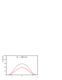
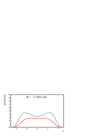
Figure 8: Rapidity distribution of the exclusively produced $Z^{0}$ for the Tevatron (left) and LHC (right) energies. The black thin solid line corresponds to Born amplitudes and the grey thick solid line (red on-line) includes absorption effects.

Figure 9: The influence of different flavours on rapidity distributions of $Z^{0}$ for Tevatron (left) and LHC (right) energies. The dotted line includes: u+d+s, the dashed line u+d+s+c and the solid line: u+d+s+c+b.

The cross sections at the Tevatron energy $\sqrt{s}$ = 1.96 TeV is rather small. Recent search for the exclusive $Z^{0}$ production CDF_Z0_exclusive has found only upper limit for this process. There is a hope that at the LHC it could be measurable. One should remember, however, that in practice one can measure either $\mu^{+}\mu^{-}$ or $e^{+}e^{-}$ pairs. This means one can expect a sizeable background from the $\gamma^{*}\gamma^{*}\to l^{+}l^{-}$ processes CDF_Z0_exclusive . In order to get rid of this type of the background some cuts could be helpful.

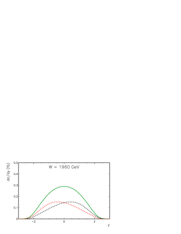
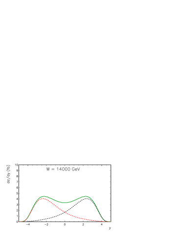
Figure 10: The photon-pomeron and pomeron-photon contributions for the Tevatron (left) and LHC (right) energies. No absorptive corrections are included here.

In Fig.11 we show transverse momentum distribution of the exclusively produced $Z^{0}$. The distribution peaks at $p_{t}\sim$ 0.3 GeV and extends to relatively large transverse momenta. This is in clear contrast to the photon-photon processes where the corresponding transverse momenta of the lepton pair would peak at much lower transverse momenta. Imposing a lower cut on the lepton pair transverse momenta would cut off the unwanted photon-photon background.

Figure 11: The transverse momentum distribution of $Z^{0}$ bosons at $\sqrt{s}$ = 1960 GeV (left) and $\sqrt{s}$ = 14 TeV (right).

There are definite plans that both ATLAS and CMS main detectors will be supplemented by several forward detectors. In principle, having two forward detectors could allow to measure two outgoing protons in coincidence. This could allow studying correlations between outgoing protons. As an example in Fig.12 we show the distribution in relative azimuthal angle between outgoing protons. Quite different distributions are obtained for the Tevatron ($\bar{p}p$ collisions) and LHC ($pp$ collisions). This effect is of the interference nature and was already discussed for exclusive $J/\Psi$ production SS07 . In contrast to the reaction with $Z^{0}$ boson the relative azimuthal angle distribution for the photon-photon processes peaks sharply at $\phi\sim$ 180^o CDF_Z0_exclusive . Therefore imposing extra cuts in the azimuthal angle space should further diminish the photon-photon background opening a chance to measure for the first time the exclusive $Z^{0}$ production in proton-proton collisions.

Figure 12: Distribution in relative azimuthal angle between outgoing protons at $\sqrt{s}$ = 1960 GeV (left) and $\sqrt{s}$ = 14 TeV (right).

Finally let us present our estimate of the inclusive double-diffractive contribution of Fig.4. In Fig.13 we show the cross section with pomeron exchanges only (dashed) and with both pomeron and reggeon exchanges included (solid). This cross sections have to be multiplied in addition by the gap survival probabilities from Table 1. In this calculation $x_{{\bf I\!P}}^{max}$ = 0.1 was assumed. This means cuts on longitudinal momentum fractions of outgoing protons/antiprotons. Even after including absorption corrections the inclusive double-pomeron contribution is a few orders of magnitude larger than the purely exclusive cross section. The rapidity distributions from Fig.13 are more narrow than the purely exclusive distributions shown earlier. This is partially related to the cuts on longitudinal momentum fractions and is of purely kinematic origin. The cross section for inclusive double pomeron contribution is certainly measurable at LHC and is bigger than the cross section for single-diffractive $Z^{0}$ production at Tevatron D0 .

Figure 13: Rapidity distributions of inclusive double-pomeron production of $Z^{0}$ boson for the Tevatron (left) and LHC (right). The solid lines include both pomeron and reggeon exchanges while the dashed lines only pomeron exchanges. In this calculation the fit (a) from Ref.H1 was used. No absorptive corrections were included here.

In Fig.14 we show two-dimensional distribution in pomeron/reggeon momentum fractions ($x_{{\bf I\!P},1},x_{{\bf I\!P},2}$). The large mass of the $Z^{0}$ boson causes that the small values of $x_{{\bf I\!P},1}$ and $x_{{\bf I\!P},2}$ are not accessible kinematically. This is more evident for the Tevatron energy. This is also the reason for much smaller cross section for double-diffractive production of $Z^{0}$ for Tevatron compared to LHC.

Figure 14: Two dimensional distributions in ($x_{{\bf I\!P},1},x_{{\bf I\!P},1}$) for the Tevatron energy W = 1960 GeV (upper panels) and for the LHC energy W = 14000 GeV (lower panels). The left panels include only pomeron exchanges while the right panels both pomeron and reggeon exchanges. In this calculation the fit (a) from Ref.H1 was used. No absorbtion corrections were included here.

VI Conclusions

We have extended the $k_{\perp}$-factorization to the exclusive production of $Z^{0}$ bosons. The production amplitude was calculated using an unintegrated gluon distribution IN_glue adjusted to inclusive deep inelastic structure functions. The so obtained $\gamma p\to Zp$ amplitude served as an input for the evaluation of the $pp\to ppZ^{0}$ process. Our results obtained with bare (i.e. without absorption) amplitudes are by a factor of 3 larger than those obtained earlier in the dipole approach. We have analyzed the role of individual flavours. For low energy it is enough to include only light flavours while at high energies all flavours must be included.

Compared to earlier works in the literature we have taken into account absorption effects. The absorption effects depend on the Z-boson rapidity and lower the cross section by a factor of 1.5-2. As for the exclusive $\Upsilon$ production RSS08 the larger rapidity, the larger the absorption effect.

Very small cross sections are obtained both for Tevatron and LHC. This means that possible background must be studied. The $Z^{0}$ is measured via $e^{+}e^{-}$ or $\mu^{+}\mu^{-}$ decay channels. Recently the CDF collaboration CDF_Z0_exclusive presented a first estimate of the upper limit for the exclusive $Z^{0}$ production at the Tevatron. Their limit is about three orders of magnitude larger than our predictions. This demonstrates difficulties to measure the exclusive process. The situation will improve at LHC (larger cross section, larger luminosity), but even there it will be rather difficult to measure the cross section.

In a detailed analysis a background from the $\gamma\gamma\to l^{+}l^{-}$ and $\gamma{\bf I\!P}\to\gamma^{*}\to l^{+}l^{-}$ (sub)processes must be taken into account. We have found that distributions in $Z^{0}$ (lepton pair) transverse momentum as well as in relative azimuthal angle between outgoing protons can be very useful to separate out the background $\gamma\gamma\to l^{+}l^{-}$ processes.

To our knowledge for the first time in the literature, we have estimated inclusive double diffractive production of $Z^{0}$ using diffractive parton distributions obtained recently from the analysis of the proton diffractive structure functions/diffractive dijets performed by the H1 collaboration at HERA. We have calculated cross section assuming Regge factorization as well as inculding absorption effects leading to the factorization breaking. Rather large inclusive double-diffractive cross sections were found at LHC. A future experiments with forward instrumentation of main LHC detectors (ATLAS and ALICE) should provide new results concerning hard diffraction. This will allow to further investigate the mechanism of Regge-factorization breaking observed already for soft total single and double diffraction.

VII Acknowledgements

We are indebted to Christophe Royon and Laurent Schoeffel for providing us with the H1 parton distributions in the pomeron. This work was partially supported by the Polish Ministry of Science and Higher Education (MNiSW) under contracts MNiSW N N202 249235 and 1916/B/H03/2008/34.

VIII Appendix: Two-channel model for the absorptive corrections

Here we present the details of the two-channel model used for the evaluation of absorptive corrections to central inclusive $Z^{0}$–production. It improves over a single–channel desription by taking into account some inelastic shadowing corrections. As physical states, one would include the proton $|{p}\rangle$ and some effective low–mass states $|{N_{i}^{*}}\rangle$ with proton–quantum numbers (representing e.g. resonances and the diffractively excited $N\pi,N\pi\pi,...$ components. The multichannel eikonal will then be an operator acting on the tensor–product space of physical states $|{N_{i}N_{j}}\rangle=|{N_{i}}\rangle\otimes|{N_{j}}\rangle$, where $N_{i}=p,N^{*}$. The proton–proton $S$–matrix in this space is now given by

$$\hat{S}(\mbox{\boldmath$b$})=\exp\Big{[}-{1\over 2}\nu(s,\mbox{\boldmath$b$})\,\hat{g}\otimes\hat{g}\Big{]}\,,$$ (23)

where the opacity $\nu(s,\mbox{\boldmath$b$})$ is given by

$$\nu(s,\mbox{\boldmath$b$})=g_{pp}^{2}\,\Big{(}{s\over s_{0}}\Big{)}^{\Delta_{\bf I\!P}}\,T_{\bf I\!P}(\mbox{\boldmath$b$})\,,$$ (24)

and we stick to an oversimplified model, in which all matrix elements have the same $b$ dependence given by $T_{\bf I\!P}(\mbox{\boldmath$b$})$. The $b$-space profile was taken in the Gaussian form:

$$T_{\bf I\!P}(\mbox{\boldmath$b$})={1\over 2\pi(B_{0}+2\alpha^{\prime}\log(s/s_{0}))}\exp\Big{[}{-\mbox{\boldmath$b$}^{2}\over 2(B_{0}+2\alpha^{\prime}\log(s/s_{0}))}\Big{]}\;.$$ (25)

The values of the bare pomeron parameters $g_{pp}^{2},\Delta_{\bf I\!P}$ as well as the parametrisation of $T_{\bf I\!P}(\mbox{\boldmath$b$})$ are given below. Notice that below, we do not distinguish between protons and antiprotons, and will always refer to proton–proton scattering even when discussing results for the Tevatron.

In the two–channel case, where all inelastic excitations are subsumed in a single effective state $|{N^{*}}\rangle$, the matrix $\hat{g}$ is written as

$$\hat{g}=\left(\begin{array}[]{cc}1+\delta&\gamma\\ \gamma&1-\delta\end{array}\right)\,.$$ (28)

It has the eigenvalues

$$\lambda_{1,2}=1\pm\sqrt{\delta^{2}+\gamma^{2}}\,,$$ (29)

and the physical states can be expanded into $S$–matrix eigenstates as

$$|{p}\rangle=\sum_{i}C_{i}^{p}|{i}\rangle\,,\,|{N^{*}}\rangle=\sum_{i}C_{i}^{N^{*}}|{i}\rangle\,.$$ (30)

Now we turn to the gap survival probabilty and evaluate the effective $S^{2}_{abs}(\mbox{\boldmath$b$})$ which enters Eq.(22). We distinguish different final states:

VIII.1 $pp\to p+Z^{0}X+p$

First let us the case of the proton–proton final state. Here we need to substitute

$$S^{2}_{abs}(\mbox{\boldmath$b$})\longrightarrow\Big{|}\langle{pp}|\Big{(}\hat{g}\otimes\hat{g}\Big{)}\hat{S}(\mbox{\boldmath$b$})|{pp}\rangle\Big{|}^{2}\,=\Big{|}\langle{pp}|\Big{(}\hat{g}\otimes\hat{g}\Big{)}\exp[-{1\over 2}\nu(s,\mbox{\boldmath$b$})\hat{g}\otimes\hat{g}]|{pp}\rangle\Big{|}^{2}\,.$$ (31)

To evaluate the matrix element $\langle{pp}|\dots|{pp}\rangle$, we should expand the protons into eigenstates of the $S$–matrix according to Eq.(30):

$$\langle{pp}|\Big{(}\hat{g}\otimes\hat{g}\Big{)}\hat{S}(\mbox{\boldmath$b$})|{pp}\rangle =|C^{p}_{1}|^{4}\lambda_{1}^{2}e^{-\nu\lambda_{1}^{2}/2}+|C^{p}_{2}|^{4}\lambda_{2}^{2}e^{-\nu\lambda_{2}^{2}/2}+2\,|C^{p}_{1}|^{2}|C^{p}_{2}|^{2}\lambda_{1}\lambda_{2}e^{-\nu\lambda_{1}\lambda_{2}/2}\,.$$

Here we suppressed the arguments of $\nu=\nu(s,\mbox{\boldmath$b$})$.

VIII.2 $pp\to Y_{1}+Z^{0}X+Y_{2}$

If protons in the final state cannot be measured, we need to sum over all excitations $Y_{1,2}\in\{p,N^{*}\}$, and we should substitute

$$S_{abs}^{2}(\mbox{\boldmath$b$}) \longrightarrow \sum_{Y_{1},Y_{2}}\Big{|}\langle{Y_{1}Y_{2}}|\Big{(}\hat{g}\otimes\hat{g}\Big{)}\hat{S}(\mbox{\boldmath$b$})|{pp}\rangle\Big{|}^{2}=\langle{pp}|\Big{(}\hat{g}\otimes\hat{g}\Big{)}^{2}\hat{S}^{2}(\mbox{\boldmath$b$})|{pp}\rangle$$ (33)

$$= \langle{pp}|\Big{(}\hat{g}\otimes\hat{g}\Big{)}^{2}\exp[-\nu(s,\mbox{\boldmath$b$})\hat{g}\otimes\hat{g}]|{pp}\rangle$$

$$= |C^{p}_{1}|^{4}\lambda_{1}^{4}e^{-\nu\lambda_{1}^{2}}+|C^{p}_{2}|^{4}\lambda_{2}^{4}e^{-\nu\lambda_{2}^{2}}+2\,|C^{p}_{1}|^{2}|C^{p}_{2}|^{2}(\lambda_{1}\lambda_{2})^{2}e^{-\nu\lambda_{1}\lambda_{2}}\,.$$

Equivalent equations can be found in KMR_eikonal , who we largely follow in choosing $\gamma=0.55,\delta=0$. Then

$$|{p}\rangle={1\over\sqrt{2}}\Big{(}|{1}\rangle+|{2}\rangle\Big{)}\,,\,|{N^{*}}\rangle={1\over\sqrt{2}}\Big{(}|{1}\rangle-|{2}\rangle\Big{)}\,,$$ (34)

with eigenvalues $\lambda_{1,2}=(1\pm\gamma)$. The bare Pomeron parameters used in the parametrisation of the opacity (24) with $s_{0}=1\,\mathrm{GeV}^{2}$, are taken as

$$g_{pp}^{2}=27\,\mathrm{mb}\,,\,\Delta_{\bf I\!P}=0.11\,,\,B_{0}=9\,\mathrm{GeV}^{-2}\,,\,\alpha^{\prime}=0.14\,\mathrm{GeV}^{-2}\,\,.$$ (35)

These parameters are so adjusted, that we obtain reasonable values for the total cross section $\sigma_{tot}$, the elastic cross section $\sigma_{el}$, as well as the elastic slope $B_{el}$. They are obtained from

$$\sigma_{tot}=2\,\int d^{2}\mbox{\boldmath$b$}\,\Gamma(\mbox{\boldmath$b$})\,\,,\,\sigma_{el}=\int d^{2}\mbox{\boldmath$b$}\,\Gamma^{2}(\mbox{\boldmath$b$})\,\,,\,B_{el}={1\over 2}{\int d^{2}\mbox{\boldmath$b$}\,\mbox{\boldmath$b$}^{2}\Gamma(\mbox{\boldmath$b$})\over\int d^{2}\mbox{\boldmath$b$}\,\Gamma(\mbox{\boldmath$b$})}\,,$$ (36)

where the impact–parameter space forward amplitude $\Gamma(\mbox{\boldmath$b$})$ is given by

$$\Gamma(\mbox{\boldmath$b$})=1-\langle{pp}|\hat{S}(\mbox{\boldmath$b$})|{pp}\rangle\,.$$ (37)

For the energy of Tevatron Run I, $\sqrt{s}=1800\,\mathrm{GeV}$, we obtain $\sigma_{tot}=78.5\,\mathrm{mb}$, $\sigma_{el}=16.7\,\mathrm{mb}$, and $B_{el}=17.2\,\mathrm{GeV}^{-2}$. For the LHC energy of $\sqrt{s}=14\,\mathrm{TeV}$, this oversimplified model predicts $\sigma_{tot}=106\,\mathrm{mb}$, $\sigma_{el}=26\,\mathrm{mb}$, and $B_{el}=19.8\,\mathrm{GeV}^{-2}$.

References

• (1) T. Aaltonen et al. [CDF Collaboration], Phys. Rev.  D 77, 052004 (2008) [arXiv:0712.0604 [hep-ex]].
• (2) T. Aaltonen et al. [CDF Collaboration], arXiv:0902.1271 [hep-ex].
• (3) A. D. Martin, M. G. Ryskin and V. A. Khoze, arXiv:0903.2980 [hep-ph].
• (4) M. G. Albrow et al. [FP420 R and D Collaboration], arXiv:0806.0302 [hep-ex]; R. Schicker, AIP Conf. Proc.  1105, 136 (2009) [arXiv:0812.3123 [hep-ex]].
• (5) W. Schäfer and A. Szczurek, Phys. Rev.  D 76, 094014 (2007).
• (6) A. Rybarska, W. Schäfer and A. Szczurek, Phys. Lett.  B 668, 126 (2008) [arXiv:0805.0717 [hep-ph]].
• (7) V. P. Goncalves and M. V. T. Machado, Eur. Phys. J.  C 56, 33 (2008) [arXiv:0710.4287 [hep-ph]].
• (8) L. Motyka and G. Watt, Phys. Rev.  D 78, 014023 (2008) [arXiv:0805.2113 [hep-ph]].
• (9) I. P. Ivanov, N. N. Nikolaev and A. A. Savin, Phys. Part. Nucl.  37, 1 (2006).
• (10) T. Aaltonen et al. [CDF Collaboration], arXiv:0902.2816 [hep-ex].
• (11) P. Bruni and G. Ingelman, Phys. Lett. B311 (1993) 317; L. Alvero, J.C. Collins, J. Terron and J.J. Whitmore, Phys. Rev. D59 (1999) 074022.
• (12) A. G. Shuvaev, K. J. Golec-Biernat, A. D. Martin and M. G. Ryskin, Phys. Rev.  D 60, 014015 (1999).
• (13) N. N. Nikolaev and B. G. Zakharov, Z. Phys.  C 49, 607 (1991).
• (14) B. Z. Kopeliovich, J. Nemchick, N. N. Nikolaev and B. G. Zakharov, Phys. Lett.  B 309, 179 (1993) [arXiv:hep-ph/9305225].
• (15) I. P. Ivanov and N. N. Nikolaev, Phys. Rev.  D 65, 054004 (2002).
• (16) A. Aktas et al. [H1 Collaboration], Eur. Phys. J.  C 46, 585 (2006).
• (17) S. Donnachie, G. Dosch, P. Landshoff and O. Nachtmann, ”Pomeron Physics and QCD”, Cambridge University Press, Cambridge 2002.
• (18) F. Abe et al. [CDF Collaboration], Phys. Rev. D50, 5518 (1994).
• (19) G. Ingelman and P. E. Schlein, Phys. Lett.  B 152, 256 (1985).
• (20) V. Barger and R. Phillips, ”Collider Physics”, Addison-Wesley Publishing Company, Redwood Cite, 1987.
• (21) A. Aktas et al. [H1 Collaboration], Eur. Phys. J.  C 48, 715 (2006) [arXiv:hep-ex/0606004].
• (22) W. Schäfer, arXiv:hep-ph/9806295, in: Deep Inelastic Scattering and QCD: DIS 98: Proceedings. Edited by Gh. Coremans and R. Roosen. Singapore, World Scientific, 1998.
• (23) J. D. Bjorken, Phys. Rev.  D 47, 101 (1993).
• (24) K. A. Ter-Martirosyan, Sov. J. Nucl. Phys.  10, 600 (1970) [Yad. Fiz.  10, 1047 (1969)].
• (25) V. A. Khoze, A. D. Martin and M. G. Ryskin, Eur. Phys. J.  C 18, 167 (2000) [arXiv:hep-ph/0007359].
• (26) U. Maor, AIP Conf. Proc.  1105, 248 (2009) [arXiv:0811.2636 [hep-ph]].
• (27) M. Kłusek, W. Schäfer and A. Szczurek, Phys. Lett.  B 674, 92 (2009) [arXiv:0902.1689 [hep-ph]].
• (28) V. M. Abazov et al. [D0 Collaboration], Phys. Lett.  B 574, 169 (2003) [arXiv:hep-ex/0308032].