Effelsberg 100-m polarimetric observations of a sample of Compact Steep-Spectrum sources

Abstract

Aims. We completed observations with the Effelsberg 100-m radio telescope to measure the polarised emission from a complete sample of Compact Steep-Spectrum sources and improve our understanding of the physical conditions inside and around regions of radio emission embedded in dense interstellar environments.

Methods. We observed the sources at four different frequencies, namely 2.64 GHz, 4.85 GHz, 8.35 GHz, and 10.45 GHz, making use of the polarimeters available at the Effelsberg telescope. We complemented these measurements with polarisation parameters at 1.4 GHz derived from the NRAO VLA Sky Survey. Previous single dish measurements were taken from the catalogue of Tabara and Inoue.

Results. The depolarisation index DP was computed for four pairs of frequencies. A drop in the fractional polarisation appeared in the radio emission when observing at frequencies below $\sim$2 GHz. Rotation measures were derived for about 25% of the sources in the sample. The values, in the source rest frame, range from about –20 rad m^-2 found for 3C138 to 3900 rad m^-2 in 3C119. In all cases, the $\lambda^{2}$ law is closely followed.

Conclusions. The presence of a foreground screen as predicted by the Tribble model or with “partial coverage” as defined by ourselves can explain the polarimetric behaviour of the CSS sources detected in polarisation by the present observations. Indication of repolarisation at lower frequencies was found for some sources. A case of possible variability in the fractional polarisation is also suggested. The most unexpected result was found for the distribution of the fractional polarisations versus the linear sizes of the sources. Our results appear to disagree with the findings of Cotton and collaborators and Fanti and collaborators for the B3-VLA sample of CSS sources, the so-called “Cotton effect”, i.e., a strong drop in polarised intensity for the most compact sources below a given frequency. This apparent contradiction may, however, be caused by the large contamination of the sample by quasars with respect to the B3-VLA.

1 Introduction

Measurements of the polarised emission from Giga-Hertz-Peaked Spectrum (GPS) and Compact Steep-Spectrum (CSS) sources can provide important information about the physical conditions inside and around the region of radio emission. GPS/CSS sources are physically small objects with radio sizes smaller than 1 kpc (essentially on the Narrow Line Region size scale) and 15 kpc, respectively, that reside inside their host galaxies. The most widely accepted interpretation is that GPS/CSS galaxies are young radio sources (of ages $<10^{6}$ yr, Fanti et al. 1990). This view is supported by measurements of hot spot advance speeds (e.g., Polatidis & Conway 2003) and by means of spectral ageing studies (Murgia et al. 1999). GPS sources, which are the youngest, will grow into CSS and eventually into classical extended radio sources. Consequently, the measurement of the physical properties of GPS and CSS sources can provide insight into the conditions at the birth of a powerful radio source and those of sources developing in dense interstellar environments (see Fanti et al. 1995 and Readhead et al. 1996). The observations suggest that intrinsic distorsions in CSS sources are be caused by their interactions with dense and inhomogeneous gaseous environments. Asymmetries in terms of flux density, arm ratio, spectral index, and polarisation suggest that they are expanding through the dense inhomogeneous interstellar medium of their host galaxies (e.g., Saikia et al. 2003; Rossetti et al. 2006).

An effect on the synchrotron polarised emission produced by this magnetized thermal plasma is Faraday rotation, which is proportional to the product of electron density and the magnetic field component parallel to the direction of propagation integrated along the line of sight. The Rotation Measure (RM) is the amount of Faraday rotation expressed in rad m^-2. The Faraday rotation can unambiguously be determined from observations for at least three different wavelengths. Strong variations in Faraday rotation across the telescope beam will reduce or depolarise the observed fractional polarisation. This effect can often completely depolarise regions of emission.

In many sources, the polarisation increases with increasing frequency when observed at similar angular resolutions. The fractional polarisations of CSS sources at 15 GHz (6–7 %) indeed tend to be higher than at 5 GHz (1–3 %; van Breugel et al. 1984; Saikia et al. 1987). This suggests that large Faraday depths are responsible for the depolarisation between 15 GHz and 5 GHz rather than magnetic field geometry.

The magnetized plasma responsible for Faraday rotation and depolarisation can be situated either within the source, in a foreground screen, or in both. However, there are several indications, such as the magnitudes of the RMs, the total rotation of the electric vector position angle $>90^{\circ}$ without very high depolarisation, and the lack of correlation between high RMs in extragalactic sources and Galactic latitude (see for example the observations of Cygnus A by Dreher et al. 1987), that most of the observable effects are not internal to the source, but are produced in foreground material in the vicinity of the radio synchrotron source (e.g., Leahy 1990).

A model to describe the depolarisation behaviour in external screens has been discussed by Burn (1966) and later generalized by Tribble (1991) who considered the importance of the sizes of the individual Faraday cells in relation to the observing beam sizes. A variation in the ratio of these sizes can cause a more or less strong decline in the intrinsic polarisation percentage towards longer wavelengths. A successful application of the Tribble model, which implies the existence of a foreground screen, can be found in Fanti et al. (2004), who analysed multi-frequency observations of the B3-VLA CSS sources (Fanti et al. 2001).

Many GPS/CSS sources have been observed mainly with radio interferometers. These investigations have provided very interesting results about the polarised state of the radio emission in GPS/CSS sources. A summary can be found in O’Dea (1998) and Cotton et al. (2003). However, apart from the B3-VLA sample (Fanti et al. 2001), most of the samples observed in polarisation so far (Lüdke et al. 1998; Akujor et al. 1995; van Breugel et al. 1984; Rossetti et al. 2008) contained subsets of sources whose incompleteness hamper statistical studies or which were observed at a single or dual frequency.

The set up of this paper is as follows. Sample selection, observations and data reduction are described in Sect. 2. Results from the observations are presented in Sect. 3 and discussed in Sect 4. In Sect. 5 we draw our conclusions. Plots of the fractional polarisation $m$ and Rotation Measures RM versus wavelength squared are compiled in Appendix 1. Comments about individual sources can be found in Appendix 2.

2 Observations and data reduction

2.1 The sample

The sample of CSS sources subject to the present investigation was constructed by Fanti et al. (1990) from the 3CR catalogue (Jenkins et al. 1977) and the Peacock & Wall (1982, hereafter PW) sample. Since there is enough information about the radio structures and the spectral behaviour of the sources in the 3CR and PW catalogues, it is safe to assume that the sample contains all the CSS sources belonging to those catalogues with projected linear sizes less than 15 kpc, flux density at 178 MHz $\geq$ 10 Jy, log P${}_{178}>$26.5 W Hz^-1, and with $|b|>10^{\circ},\delta>10^{\circ}$, and can thus be considered statistically complete.

We observed all the sources belonging to this sample with the Effelsberg 100-m radio telescope at four frequencies between 2.64 GHz and 10.45 GHz in a relatively short period of time (i.e., contemporaneously at the three higher frequencies, and 16 months later at 2.64 GHz). We choose this approach to avoid time variability effects when measuring the percentage of polarised flux density for each of these sources, the depolarisation indices, and the RMs with the aim of understanding more clearly the physical conditions in which CSS sources eventually expand to become larger sources.

Polarisation parameters at 1.4 GHz were also derived for the full sample from the National Radio Astronomy Observatory Very Large Array Sky Survey (NVSS; Condon et al. 1998). Because of their small angular sizes, CSS sources are point-like at the NVSS resolution. In the analysis of sources that were found polarised at two or more of the five frequencies above, we complemented the polarisation measurements with those listed by Tabara & Inoue (1980).

For consistency with previous work, we used the cosmology H${}_{0}=100$ km s^-1 Mpc^-1 and q${}_{0}=0.5$.

2.2 Observations

The Effelsberg 100-m telescope was used to observe the complete sample of GPS/CSS sources constructed by Fanti et al. (1990). To minimize the occurrence of possible n$\pi$ ambiguities in the determination of RMs, we observed the sources at four independent frequencies, namely 2.64 GHz, 4.85 GHz, 8.35 GHz, and 10.45 GHz, making use of the polarimeters available at the Effelsberg telescope. The observations were carried out in the period January 26 to February 1, 2005 at 4.85 GHz, 8.35 GHz, and 10.45 GHz and June 24 to 26, 2006 at 2.64 GHz. Since all the target sources are point-like to the Effelsberg telescope beams, we used cross-scanning to determine the total intensity and polarisation characteristics. All sources in the sample are very bright, thus standard cross-scans along the azimuth and elevation axes were used, with 4 to 8 subscans, according to the source flux densities. Table 1 summarises the observing parameters. For further details about the observation mode and a description of the receivers, we refer to Montenegro–Montes et al. (2008), Klein et al. (2003), and references therein.

Table 1: Observing parameters and estimated integration times

Centre Frequency [GHz]	2.64	4.85	8.35	10.45
Bandwidth [MHz]	80	500	1100	300
System Temp.(zenith) [K]	17	27	22	53
Scan length [′]	16	12	8	6
Scan speed [′/min]	45	45	40	30

The calibration sources 3C 286 and 3C 295 were regularly observed to correct for time-dependent gain instabilities and to bring our measurements onto an absolute flux density scale (Baars et al. 1977). The quasar 3C 286 was also used as a polarisation calibrator to obtain the polarisation degree $m$ and the polarisation angle $\chi$ in agreement with values in the literature (Tabara et al. 1980). The unpolarised planetary nebula NGC 7027 was also observed to estimate the instrumental polarisation. We found an instrumental polarisation ($p_{instr}$) of 0.5% at 2.64 GHz, 0.5% at 4.85 GHz, 0.3% at 8.35 GHz, and 0.8% at 10.45 GHz.

The measurement of flux densities from the single-dish cross-scans was done by fitting Gaussians to the signal of the polarimeter output channels (Stokes I, Q and U) and identifying the Gaussian amplitudes with the flux densities $S_{I}$, $S_{Q}$, and $S_{U}$. For all sources with significant $S_{Q}$ and $S_{U}$ contributions, the polarised flux density $S_{P}$, the degree of linear polarisation $m$, and the polarisation angle $\chi$ were computed.

We consider three main contributions to the flux density error as in Klein et al. (2003). These are

(i) the calibration error $\Delta S_{c}$, which is estimated to be the dispersion in the different observations of the flux density calibrators, i.e., about 2% at all observing frequencies;

(ii) the error introduced by noise, $\Delta S_{i}\sim$2 mJy (i = I,Q,U), which is estimated from the noise at the scan edges;

(iii) the confusion error $\Delta S_{conf}$ caused by background sources within the beam area, estimated to be 1.5 mJy at 2.64 GHz, 0.45 mJy at 4.85 GHz, 0.17 mJy at 8.35 GHz, and 0.08 mJy at 10.45 GHz (Klein et al. 2003; the value at 8.35 GHz was extrapolated from these existing measurements. The confusion limits can be neglected in the calculation of the total error in Stokes $Q$ and $U$.

These contribute to the total error in the following way:

$$\Delta S_{\it i}=\sqrt{(S_{\it i}*\Delta S_{c})^{2}+\Delta S_{\it i}^{2}+\Delta S_{conf}^{2}}$$

Since we are dealing with relatively bright targets, instrumental polarisation is an issue in many cases. This has been included in the error of the fractional polarisation in the following way:

$$\Delta S_{P}=\sqrt{\frac{(S_{Q}*\Delta S_{Q})^{2}+(S_{U}*\Delta S_{U})^{2}}{S_{P}^{2}}+(p_{instr}*S_{I})^{2}}$$

For all other errors we follow the definitions given by Klein et al. (2003). The errors associated with the position angles $\chi$ also account for the distribution, assumed to be Gaussian, in the values of $\chi$ obtained for the calibrator 3C286 in the calibration process.

2.3 Archival data

The Effelsberg measurements were complemented with data of the NRAO VLA Sky Survey (NVSS) at 1.4 GHz (Condon et al. 1998). In all these measurements, our targets are point-like to the corresponding beams, thus beam depolarising effects are avoided. The polarised flux densities in Table 2 are given for sources with polarised flux densities greater than three times the rms error. The rms uncertainty is computed following Eq. 49 in Condon et al. (1998)

$$\sigma_{P}^{2}\approx 2\sigma_{Q,U}^{2}+\epsilon_{P}^{2}A_{P}^{2}$$

where $\epsilon_{P}^{2}$ is the residual instrumental polarisation, which is about 0.12% for a large sample of sources stronger than 1 Jy and $A_{P}$ is the fitted peaked amplitude. In Table 3, we report the fractional polarisation values for these sources.

Table 2: Flux densities and polarised flux densities from Effelsberg 100-m and NVSS measurements.

Name		S1.4			S2.64			S4.85			S8.35			S10.45			Sp1.4			Sp2.64			Sp4.85			Sp8.35			Sp10.45
		[mJy]			[mJy]			[mJy]			[mJy]			[mJy]			[mJy]			[mJy]			[mJy]			[mJy]			[mJy]
3C43	0127+23	29414	$\pm$	88	1787	$\pm$	37	1109	$\pm$	22	698	$\pm$	14	578	$\pm$	12		$<$10.8			$<$ 38.4			$<$6.6		14.7 $\pm$ 4.1			12.2$\pm$ 2.3
3C48	0134+32	16018	$\pm$	481	9373	$\pm$	191	5534	$\pm$	113	3243	$\pm$	65	2495	$\pm$	52	70.8 $\pm$ 57.6				$<$195.0		185.5 $\pm$ 43.1			160.5 $\pm$ 18.8			139.5 $\pm$5.6
3C49	0138+13	2740	$\pm$	82	1552	$\pm$	33	878	$\pm$	18	494	$\pm$	10	376	$\pm$	8		$<$9.9			$<$ 34.5			$<$20.4			$<$8.7			$<$ 6.3
3C67	0221+27	3024	$\pm$	91	1757	$\pm$	36	997	$\pm$	20	575	$\pm$	12	419	$\pm$	9	17.0 $\pm$ 10.9				$<$ 37.8			$<$23.4		22.3 $\pm$ 3.4			15.7$\pm$ 1.9
4C34.07	0223+34	2894	$\pm$	87	2483	$\pm$	51	2234	$\pm$	46	1452	$\pm$	30	1212	$\pm$	25		$<$10.5			$<$ 51.6			$<$52.2			$<$24.9			$<$13.2
4C16.09	0316+16	8028	$\pm$	241	5038	$\pm$	103	2937	$\pm$	60	1563	$\pm$	32	1187	$\pm$	25		$<$28.9			$<$103.5			$<$6.9			$<$27.0			$<$12.9
	0319+12	1907	$\pm$	67	1704	$\pm$	35	1791	$\pm$	37	1527	$\pm$	31	1549	$\pm$	32	71.8$\pm$ 7.0			95.3 $\pm$ 12.3			113.0$\pm$ 14.1			88.9 $\pm$ 8.9			77.2$\pm$ 5.7
3C93.1	0345+33	2365	$\pm$	71	1390	$\pm$	29	926	$\pm$	19	477	$\pm$	10	383	$\pm$	8		$<$8.6			$<$ 30.0			$<$21.6			$<$8.4		9.1$\pm$ 1.6
4C76.03	0404+76	5619	$\pm$	169	4042	$\pm$	83	3355	$\pm$	69	2087	$\pm$	42	1648	$\pm$	34		$<$20.3			$<$ 83.4			$<$78.3			$<$36.0			$<$18.0
	0428+20	3755	$\pm$	112	3166	$\pm$	65	2761	$\pm$	57	1542	$\pm$	31	1289	$\pm$	26		$<$13.6			$<$ 65.7			$<$64.5			$<$26.7			$<$14.1
3C119	0429+41	9832	$\pm$	295	6126	$\pm$	126	4722	$\pm$	97	2677	$\pm$	54	2260	$\pm$	47		$<$35.4			$<$125.4			$<$110.1		157.9 $\pm$ 15.7			200.6$\pm$ 8.9
3C138	0518+165	8603	$\pm$	258	5780	$\pm$	119	4119	$\pm$	84	2552	$\pm$	53	2160	$\pm$	45	619.0 $\pm$ 31.0			595.5$\pm$ 41.0			411.6 $\pm$ 32.8			297.8 $\pm$ 17.6			218.8$\pm$8.8
3C147	0538+49	22880	$\pm$	686	13436	$\pm$	276	10120	$\pm$	207	4735	$\pm$	96	3823	$\pm$	80		$<$82.3			$<$274.5			$<$236.1			$<$81.6		47.3 $\pm$ 13.6
3C186	0740+38	1236	$\pm$	37	615	$\pm$	14	271	$\pm$	8	114	$\pm$	3	85	$\pm$	3		$<$4.6			$<$ 15.3			$<$6.3			$<$2.4			$<$ 3.0
3C190	0758+14	2734	$\pm$	82	1359	$\pm$	28	746	$\pm$	16	426	$\pm$	10	360	$\pm$	8		$<$9.9			$<$ 31.5			$<$17.4			$<$7.8			$<$ 5.1
3C216	0906+43	4239	$\pm$	127	1446	$\pm$	50	1731	$\pm$	35	1413	$\pm$	29	1337	$\pm$	29		$<$15.3			$<$ 52.5			$<$40.5			$<$24.3			$<$14.7
3C237	1005+07	6522	$\pm$	196	3608	$\pm$	74	1971	$\pm$	42	1034	$\pm$	21	823	$\pm$	17		$<$23.5			$<$ 76.5			$<$45.9			$<$18.0		9.7$\pm$ 3.2
3C241	1019+22	1686	$\pm$	51	799	$\pm$	17	350	$\pm$	7	161	$\pm$	33	112	$\pm$	3		$<$6.2			$<$ 19.5			$<$8.1			$<$3.0			$<$ 1.2
4C31.38	1153+31	2978	$\pm$	89	1751	$\pm$	36	1030	$\pm$	21	545	$\pm$	11	441	$\pm$	10		$<$10.8			$<$ 45.0			$<$24.0			$<$9.6		8.6$\pm$ 1.8
3C268.3	1203+64	3719	$\pm$	112	1947	$\pm$	39	1153	$\pm$	23	618	$\pm$	13	479	$\pm$	10		$<$13.4			$<$ 40.8			$<$27.0		17.2 $\pm$ 3.7			14.2$\pm$ 2.1
	1225+36	2098	$\pm$	63	1434	$\pm$	30	753	$\pm$	16	353	$\pm$	9	239	$\pm$	5		$<$7.7			$<$ 31.5			$<$17.7			$<$6.3			$<$2.4
3C277.1	1250+56	2288	$\pm$	69	1343	$\pm$	30	790	$\pm$	16	481	$\pm$	10	384	$\pm$	8		$<$8.3			$<$ 29.4			$<$18.3		14.3 $\pm$ 2.9			9.9$\pm$ 1.8
4C32.44	1323+32	4862	$\pm$	146	3369	$\pm$	70	2293	$\pm$	47	1540	$\pm$	31	1293	$\pm$	28		$<$17.5		17.3 $\pm$ 2.3				$<$53.4			$<$26.7			$<$14.1
3C286	1328+30	14902	$\pm$	447	10607	$\pm$	219	7430	$\pm$	152	5179	$\pm$	104	4474	$\pm$	94	999.9 $\pm$ 53.7			1152.7$\pm$ 74.1			776.7 $\pm$ 59.4			607.4 $\pm$ 31.5			525.8$\pm$ 18.4
3C287	1328+27	7052	$\pm$	212	4697	$\pm$	97	3130	$\pm$	64	2050	$\pm$	42	1748	$\pm$	36	45.6 $\pm$ 25.4			168.7$\pm$ 32.3			116.6 $\pm$ 24.4			65.2 $\pm$ 11.8			58.6$\pm$ 6.4
4C62.22	1358+62	4308	$\pm$	129	2765	$\pm$	57	1701	$\pm$	35	1080	$\pm$	22	888	$\pm$	18		$<$15.6			$<$ 57.3			$<$39.6			$<$18.6			$<$9.9
	1413+34	1864	$\pm$	56	1488	$\pm$	30	1059	$\pm$	22	735	$\pm$	15	621	$\pm$	14		$<$6.8		45.8 $\pm$ 11.2				$<$24.6			$<$12.9			$<$7.5
3C298	1416+06	6100	$\pm$	183	2888	$\pm$	60	1432	$\pm$	30	789	$\pm$	17	616	$\pm$	14		$<$22.0			$<$ 60.0			$<$33.3		14.6 $\pm$ 4.6			12.8 $\pm$ 2.6
3C299	1419+41	3147	$\pm$	111	1721	$\pm$	35	922	$\pm$	20	502	$\pm$	10	400	$\pm$	9		$<$11.4			$<$ 40.8			$<$21.6			$<$9.0			$<$6.6
OQ172	1442+10	2418	$\pm$	72	1398	$\pm$	38	1032	$\pm$	21	641	$\pm$	14	516	$\pm$	11	31.7$\pm$ 8.8			63.2 $\pm$ 12.0			26.5 $\pm$ 8.0			14.2 $\pm$ 3.8				$<$8.7
3C303.1	1443+77	1880	$\pm$	66	882	$\pm$	19	413	$\pm$	8	199	$\pm$	4	128	$\pm$	3		$<$6.9			$<$ 20.1			$<$9.6			$<$3.9			$<$2.4
3C305.1	1447+77	1666	$\pm$	50	837	$\pm$	18	412	$\pm$	9	208	$\pm$	4	154	$\pm$	3		$<$6.2			$<$ 20.1			$<$9.6			$<$11.7			$<$3.9
3C309.1	1458+71	7468	$\pm$	224	5129	$\pm$	105	3552	$\pm$	73	2568	$\pm$	52	2196	$\pm$	46	91.1 $\pm$ 26.9			188.3 $\pm$ 35.2			8.5 $\pm$ 2.8			70.8 $\pm$14.8			55.5 $\pm$ 8.8
3C318	1517+20	2688	$\pm$	81	1417	$\pm$	29	764	$\pm$	16	417	$\pm$	8	322	$\pm$	7		$<$9.8			$<$ 30.9		25.8 $\pm$ 6.0			27.6 $\pm$ 2.6			29.6 $\pm$ 1.8
	1600+33	2991	$\pm$	90	1980	$\pm$	41	1433	$\pm$	29	1049	$\pm$	21	915	$\pm$	20		$<$10.8			$<$ 42.3			$<$33.3			$<$18.3			$<$10.5
OS111	1607+26	4908	$\pm$	147	3140	$\pm$	65	1728	$\pm$	35	902	$\pm$	18	681	$\pm$	15		$<$17.7			$<$ 98.7			$<$40.2			$<$15.6			$<$8.1
3C343	1634+62	5002	$\pm$	150	2858	$\pm$	59	1503	$\pm$	31	808	$\pm$	16	622	$\pm$	13		$<$18.0			$<$ 59.1			$<$35.1			$<$14.1		8.4 $\pm$ 2.5
3C343.1	1637+62	4611	$\pm$	138	2384	$\pm$	49	1190	$\pm$	24	631	$\pm$	13	479	$\pm$	10		$<$16.6			$<$ 49.2			$<$27.9			$<$11.1			$<$6.0
3C346	1641+17	3666	$\pm$	110	2260	$\pm$	47	1426	$\pm$	29	915	$\pm$	19	773	$\pm$	17	80.6 $\pm$ 13.3				$<$ 47.7			$<$33.3			$<$45.9		13.8 $\pm$ 3.0
4C39.56	1819+39	3507	$\pm$	105	1871	$\pm$	42	938	$\pm$	19	463	$\pm$	10	337	$\pm$	7		$<$12.7			$<$ 39.9			$<$21.9			$<$8.1			$<$4.5
3C380	1828+48	13573	$\pm$	413	8139	$\pm$	167	5073	$\pm$	105	3523	$\pm$	71	3055	$\pm$	63	62.2$\pm$ 49.5				$<$ 166.5			$<$118.2			$<$60.6			$<$32.7
4C29.56	1829+29	2924	$\pm$	88	1945	$\pm$	40	1168	$\pm$	24	679	$\pm$	14	533	$\pm$	12		$<$10.6			$<$ 40.8			$<$27.3			$<$12.0			$<$6.9
4C11.69	2230+11	7202	$\pm$	216	5695	$\pm$	118	4135	$\pm$	85	3396	$\pm$	69	3209	$\pm$	67	114.0 $\pm$26.0			229.6$\pm$ 39.1			147.6 $\pm$ 32.3			127.3 $\pm$ 19.6			116.4 $\pm$11.6
3C454	2249+18	2133	$\pm$	64	1265	$\pm$	26	761	$\pm$	16	469	$\pm$	10	383	$\pm$	8	77.4 $\pm$ 7.8			73.6$\pm$ 9.1			71.0 $\pm$ 6.1			52.7 $\pm$ 2.9			42.8 $\pm$ 1.9
3C454.1	2248+71	1555	$\pm$	47	696	$\pm$	15	287	$\pm$	6	119	$\pm$	3	87	$\pm$	2		$<$5.8			$<$ 16.8			$<$6.9			$<$3.6			$<$0.9
3C455	2252+12	2706	$\pm$	81	1491	$\pm$	30	772	$\pm$	16	421	$\pm$	93	312	$\pm$	7	55.8 $\pm$ 9.9			50.5$\pm$ 10.9				$<$18.0			$<$7.8		4.7$\pm$ 1.5
	2342+82	3777	$\pm$	113	2275	$\pm$	47	1308	$\pm$	27	747	$\pm$	15	579	$\pm$	12		$<$13.7			$<$ 47.4			$<$30.6			$<$13.2			$<$6.6

3 Results from the observations

In Table 2, we present both total and polarised flux densities derived by analysing the results of the observations completed with the Effelsberg 100-m radio telescope at the four frequencies plus those extracted from the NVSS. These measurements plus those derived from the literature are shown in Appendix 1.

3.1 Percentage of polarised emission

The sample constructed by Fanti et al. (1990) contains 47 sources. We considered them to be polarised when the intensity of the polarised emission is 3 times the rms error estimated source by source for the polarised emission. This provides in general lower limits of 3% at 2.64 GHz, 2% at 4.85 GHz, 1% at 8.35 GHz, and 1% at 10.45 GHz. Table 3 summarizes the values of the polarisation parameters for sources with polarised flux densities above the detection limits.

A high fraction of sources have polarised emission, if any, below the detection limits of our Effelsberg observations. We found that 22 of them are polarised at 10.45 GHz, 16 sources are polarised at 8.35 GHz, 10 sources are polarised at 4.85 GHz, and 10 sources are polarised at 2.64 GHz. The number of sources with detected polarised emission clearly decreases from high to low frequency. The percentage of polarised emission $m$ ranges between $\sim$6% and $\sim$12% for the most polarised sources 3C138, 3C286, and 3C454.

Because most of the sources in the sample have polarised emission below the detection limits of our observations, the median values of $m$ for the entire sample are below 3% at 2.64 GHz, below 2% at 4.85 GHz, below 1% at both 8.35 GHz and 10.45 GHz, and below 1.58% at 1.4 GHz.

Table 3: Percentage of polarised flux density and position angle of the electric vector at the five frequencies.

Name		$LS$	$m_{1.4}$	$m_{2.64}$	$m_{4.85}$	$m_{8.35}$	$m_{10.45}$	$\chi_{1.4}$	$\chi_{2.64}$	$\chi_{4.85}$	$\chi_{8.35}$	$\chi_{10.45}$
		[kpc]	[$\%$]	[$\%$]	[$\%$]	[$\%$]	[$\%$]	[deg]	[deg]	[deg]	[deg]	[deg]
3C43	0127+23	12.85				2.1$\pm$0.6	2.1$\pm$0.4				2$\pm$2	13$\pm$3
3C48	0134+32	4.00	0.44$\pm$0.12		3.4$\pm$0.8	4.9$\pm$0.6	5.6$\pm$0.4	–70.8$\pm$0.1		–78$\pm$2	–68$\pm$2	–61$\pm$2
3C49	0138+13	3.85
3C67	0221+27	6.45	0.56$\pm$0.12			3.9$\pm$0.6	3.7$\pm$0.5	59.3$\pm$0.5			62$\pm$2	62$\pm$3
4C34.07	0223+34	4.04*
4C16.09	0316+16	1.3+
	0319+12	0.2+	3.80$\pm$0.18	5.6$\pm$0.7	6.3$\pm$0.8	5.8$\pm$0.6	5.0$\pm$0.4	41.0$\pm$0.1	59$\pm$3	73$\pm$2	74$\pm$2	71$\pm$2
3C93.1	0345+33	0.7					2.4$\pm$0.4					59$\pm$3
4C76.03	0404+76	0.6+
OF247	0428+20	0.49
3C119	0429+41	0.9				5.9$\pm$0.6	8.8$\pm$0.4				49$\pm$2	179$\pm$2
3C138	0518+16	3.25	7.2$\pm$0.25	10.3$\pm$0.7	9.9$\pm$0.8	11.7$\pm$0.7	9.9$\pm$0.4	–11.1$\pm$0.0	–11$\pm$2	–13$\pm$2	–11$\pm$2	–7$\pm$2
3C147	0538+49	2.58					1.2$\pm$0.4					189$\pm$2
3C186	0740+38	5.14
3C190	0758+14	11.19
3C216	0906+43	33.44
3C237	1005+07	7.11					1.2$\pm$0.4					18$\pm$4
3C241	1019+22	3.82
4C31.38	1153+31	3.96					1.9$\pm$0.4					16$\pm$4
3C268.3	1203+64	5.28				2.8$\pm$0.6	3.0$\pm$0.4				–97$\pm$2	-98$\pm$6
ON343	1225+36	0.23+
3C277.1	1250+56	4.57				3.0$\pm$0.6	2.6$\pm$0.5				11$\pm$2	7$\pm$6
4C32.44	1323+32	0.18+
3C286	1328+30	15.81	6.70$\pm$0.23	10.9$\pm$0.7	10.8$\pm$0.8	11.7$\pm$0.7	11.7$\pm$0.5	35.0$\pm$0.0	31$\pm$2	33$\pm$2	33$\pm$2	33$\pm$2
3C287	1328+25	0.43	0.65$\pm$0.12	3.6$\pm$0.7	3.7$\pm$0.8	3.2$\pm$0.6	3.3$\pm$0.4	29.9$\pm$0.2	105$\pm$2	–32$\pm$2	–15$\pm$2	–6$\pm$2
4C62.22	1358+62	0.17+
	1413+34	0.26		3.1$\pm$0.7					199$\pm$3
3C298	1416+06	9.1				1.8$\pm$0.6	2.1$\pm$0.4				–42$\pm$3	–30$\pm$4
3C299	1419+41	36.31
OQ172	1442+10	0.1+	1.30$\pm$0.13	4.5$\pm$0.9	2.6$\pm$0.8	2.2$\pm$0.6		–86.2$\pm$0.3	212$\pm$4	69$\pm$2	76$\pm$3
3C303.1	1443+77	1.28
3C305.1	1447+77	7.86
3C309.1	1458+71	9.25	1.20$\pm$0.13	3.7$\pm$0.7	2.4$\pm$0.7	2.7$\pm$0.6	2.5$\pm$0.4	39.9$\pm$0.1	104$\pm$2	252$\pm$2	247$\pm$2	243$\pm$2
3C318	1517+20	3.25			3.4$\pm$0.8	6.6$\pm$0.6	9.2$\pm$0.6			60$\pm$2	–14$\pm$2	–24$\pm$2
	1600+33	$<$0.4
OS111	1607+26	0.19+
3C343	1634+62	11.48					1.4$\pm$0.4					–104$\pm$3
3C343.1	1637+62	1.54
3C346	1641+17	27.01	2.20$\pm$0.14				1.8$\pm$0.4	–82.7$\pm$0.1				–4$\pm$3
4C39.56	1819+39	3.20
3C380	1828+48	55.62	0.45$\pm$0.12					44.2$\pm$0.1
4C29.56	1829+29	12.40
4C11.69	2230+11	9.7	1.6$\pm$0.13	4.0$\pm$0.7	3.6$\pm$0.8	3.7$\pm$0.6	3.6$\pm$0.4	–61.1$\pm$0.1	7$\pm$2	48$\pm$2	58$\pm$2	60$\pm$2
3C454	2249+18	8.39	3.6$\pm$0.16	5.8$\pm$0.7	9.3$\pm$0.8	11.2$\pm$0.7	11.2$\pm$0.4	53.4$\pm$0.1	41$\pm$2	87$\pm$2	98$\pm$2	101$\pm$2
3C454.1	2248+71	5.5
3C455	2252+12	11.75	2.10$\pm$0.14	3.4$\pm$0.7			1.5$\pm$0.5	–7.5$\pm$0.2	149$\pm$3			151$\pm$8
	2342+82	0.72+

3.2 Depolarisation index and rotation measure

Table 4 summarizes the values of the depolarisation index and of the observed RM (RM_obs) and source rest frame RM (RM_rf = RM${}_{obs}\times(1+z)^{2}$) both given in rad m^-2. The depolarisation index DP = $m_{l}/m_{h}$, is defined to be the ratio of the percentages of polarised emission at the lower ($m_{l}$) to the higher ($m_{h}$) frequency. The present observations complemented with those taken from Tabara & Inoue (1980), allow us to determine the values of the RMs for 16 sources in the list. The observing frequencies of the Effelsberg plus NVSS observations are suitably separated for a proper determination of the RMs. In particular, they allow us to apply unambiguous $n\pi$ de-rotation to the observed polarisation E-vector position angle $\chi$ at the various frequencies. When applied, these rotations always yield a linear regression with a least squares fit very close to 1, expect for an optimal fit, for the $\lambda^{2}$ rotation. We also note that there is no significant difference between the values derived from our Effelsberg observations and those from Tabara & Inoue (1980), which were acquired about 30 years earlier.

Table 4: Depolarisation indices and RMs.

Name		z	Id	DP	DP	DP	DP	RMobs	lm-1	RMobs+TI	lm-2	RMrf
				8.35/10.45	4.85/8.35	2.64/4.85	1.4/2.64	[rad m${}^{-2}]$		[rad m-2]		[rad m-2]
3C43	0127+23	1.46	Q	1.00						$-$69	0.9965	$-$419
3C48	0134+32	0.37	Q	0.87	0.69			$-$79	0.9994	$-$64	0.9900	$-$120
3C49	0138+13	0.62	G
3C67	0221+27	0.31	G	1.05				$-$1	0.9999	$-$67	0.9945	$-$115
4C34.07	0223+34	2.91*	Q
4C16.09	0316+16	0.97*	Q									$-$249
	0319+12	2.67	Q	1.16	1.09	0.89	0.07	$-$12	0.9521	$-$19	0.7698	$-$164
3C93.1	0345+33	0.24	G
4C76.03	0404+76	0.6	G
OF247	0428+20	0.22	G
3C119	0429+41	1.023	Q	0.66						1928	0.9663	3900
3C138	0518+165	0.76	Q	1.18	0.85	1.04	0.70	$-$1	0.04	$-$6	0.8786	$-$19
3C147	0538+49	0.55	Q
3C186	0740+38	1.06	Q
3C190	0758+14	1.2	Q
3C216	0906+43	0.67	Q
3C237	1005+07	0.88	G
3C241	1019+22	1.62	G
4C31.38	1153+31	0.42	Q
3C268.3	1203+64	0.37	G	0.93						114	0.9853	213
ON343	1225+36	1.973*	Q
3C277.1	1250+56	0.32	Q	1.15						$-$59	0.9961	$-$102
4C32.44	1323+32	0.37	G
3C286	1328+30	0.85	Q	0.99	0.91	1.01	0.61
3C287	1328+25	1.06	Q	0.97	1.16	0.97	0.18	$-$148	0.9957	$-$146	0.9954	$-$618
4C62.22	1358+62	0.43	G				0.02
	1413+34
3C298	1416+06	1.44	Q	0.86						96	0.9911	573
3C299	1419+41	0.37	G
OQ172	1442+10	3.52	Q		1.18	1.73	0.29	$-$66	0.9994	$-$71	0.9376	$-$1451
3C303.1	1443+77	0.2	G
3C305.1	1447+77	1.13	G
3C309.1	1458+71	0.91	Q	1.08	0.89	1.54	0.32	60	0.9996	46	0.9830	169
3C318	1517+20	1.57	G	0.72	0.52			498	0.9987	342	0.9995	2260
	1600+33	1.1*	G?
OS111	1607+26	0.47*	G
3C343	1634+62	0.99	Q
3C343.1	1637+62	0.75	G
3C346	1641+17	0.16	G
4C39.56	1819+39	0.80	G
3C380	1828+48	0.69	Q
4C29.56	1829+29	0.84	G
4C11.69	2230+11	1.04	Q	1.03	0.97	1.10	0.40	$-$39	0.9694	$-$38	0.9894	$-$157
3C454	2249+18	1.76	Q	1.02		0.62	0.62	$-$88	1.000	$-$88	0.9997	$-$669
3C454.1	2248+71	1.84	G
3C455	2252+12	0.54	G				0.62	$-$68	0.9402	82	0.9923	194
	2342+82	0.74	Q

4 Discussion

In the following we discuss trends of the depolarisation index, the achieved values of the rotation measure, and the distribution of the percentage of polarised emission versus the linear sizes of the observed sources.

4.1 General trends

The depolarisation index DP has been computed for four pairs of frequencies. The mean and the median values of the DP are reported in Table 5.

Table 5: The mean and the median values of the depolarisation index

Depolarisation index	DPmean	DPmedian
DP8.35/10.45	0.98$\pm$0.15	1.00 ${}_{-0.03}\hskip-21.0pt\,^{+0.02}$
DP4.85/8.35	0.90$\pm$0.20	0.91 ${}_{-0.006}\hskip-25.0pt\,^{+0.18}$
DP2.64/4.85	1.11$\pm$0.33	1.01 ${}_{-0.12}\hskip-21.0pt\,^{+0.09}$
DP1.4/2.64	0.33$\pm$0.23	0.32 ${}_{-0.14}\hskip-21.0pt\,^{+0.30}$

Clearly a drop in the fractional polarisation appears in the radio emission at frequencies below $\sim$2 GHz. The number of polarised sources in our list of CSS sources drops from 46% at 10.45 GHz to 23% at 2.64 GHz, and they have a median fractional polarisation of below 2% at 5.0 GHz that agrees with previous findings (for example Saikia et al. 1987).

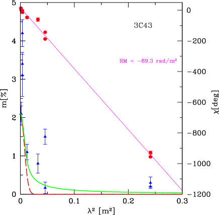
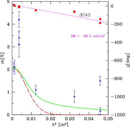
Figure 2: Position angles of the electric field vector $\chi$ in deg (dots) and fractional polarisation $m$ in % (triangles) $versus$ $\lambda^{2}$ in m² for the source 3C43, for the full range (left), and for a narrow range (right) of wavelengths. The solid line represents the Tribble model, the dashed line the Burn model.

In Fig.s 2 to 17 (Appendix 1), we plot the fractional polarisation values $m$ derived from our Effelsberg observations complemented with those extracted from the NVSS at 1.4 GHz and those taken from the Tabara & Inoue (1980) catalogue. The general trend is a quick decrease in the fractional polarisation with increasing wavelength. However, $m$ does not always drop to zero at longer wavelengths ($\lambda>$ 49 cm) as predicted by the Burn (1966) model. The Burn model (dashed line) and the Tribble (1991) model (solid line) have been plotted in Figs. 2 to 17, according to Eqs. (1) and (2) in Fanti et al. (2004). For both models, we have adopted as the intrinsic fractional polarisation $m_{0}$ the one measured by us at 10.45 GHz. For the Tribble model, which assumes RM randomly distributed and a distribution of cell sizes, the ratio of the characteristic scale representing the largest cell scale to the observing beam is taken to be equal to 1. With these assumptions, the model corresponds to the highest possible polarisation at long wavelengths, thus an upper limit to the expected fractional polarisation behaviour.

Very low fractional polarisation for sources belonging to this class is also found with interferometric observations. For example, Peck & Taylor (2000) did not detect any linear polarisation with VLBI observations at 8.35 GHz on a sample of 21 Compact Symmetric Objects (CSOs are CSS sources that exhibit core and lobe emission on each side of the core). While this strengthens the assumption that beam depolarisation plays a minor rôle it also means that the polarisation characteristics of CSS sources are not yet fully clarified.

Figure 1: Percentage of polarised emission versus source linear sizes at 8.35 GHz. Dots are Quasars; open circles are Galaxies.

4.2 Model fitting

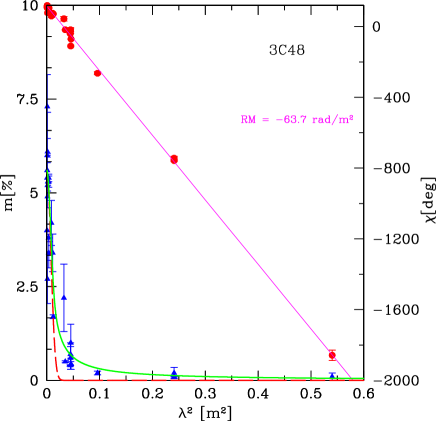
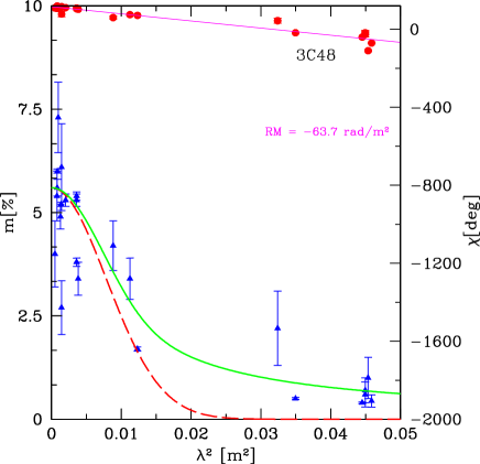
Figure 3: Position angles $\chi$ and fractional polarisation $m$ for the source 3C48. Layout as in Fig. 2.

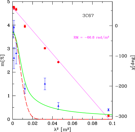
Figure 4: Position angles $\chi$ and fractional polarisation $m$ for the source 3C67. Layout as in Fig. 2.

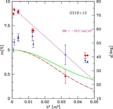
Figure 5: Position angles $\chi$ and fractional polarisation $m$ for the source 0319+12. Layout as in Fig. 2.

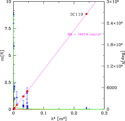
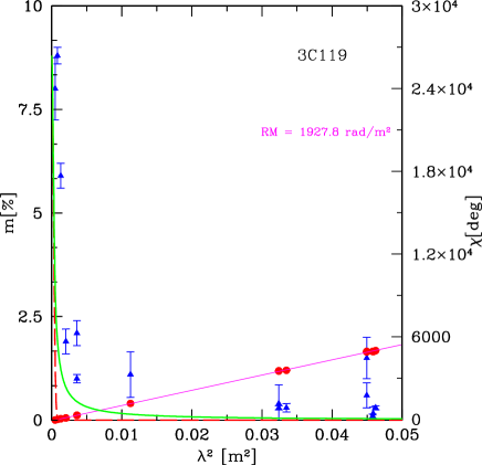
Figure 6: Position angles $\chi$ and fractional polarisation $m$ for the source 3C119. Layout as in Fig. 2.

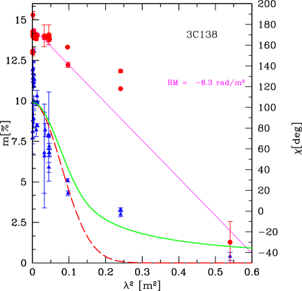
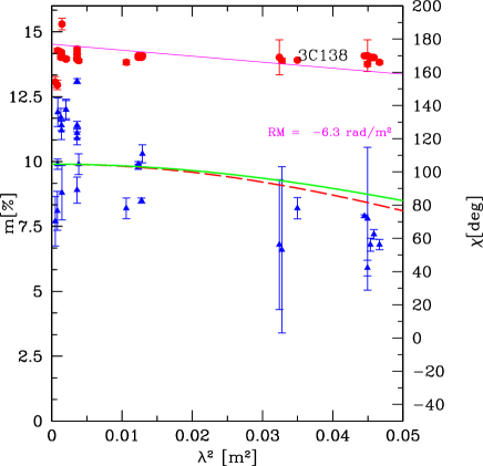
Figure 7: Position angles $\chi$ and fractional polarisation $m$ for the source 3C138. Layout as in Fig. 2.

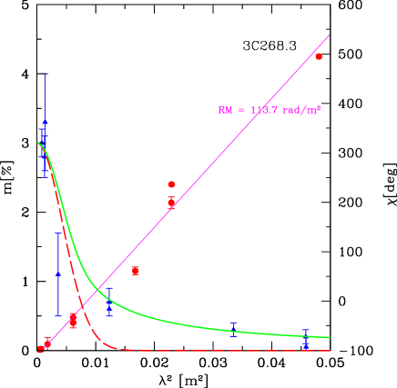
Figure 8: Position angles $\chi$ and fractional polarisation $m$ for the source 3C268.3. Layout as in Fig. 2.

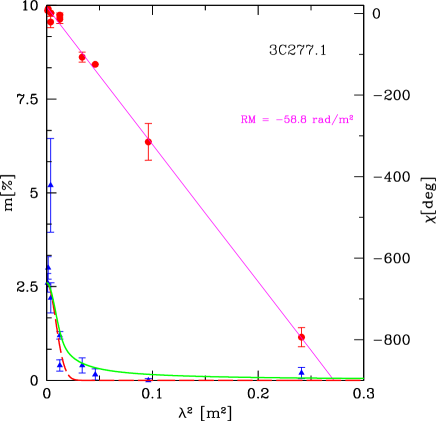
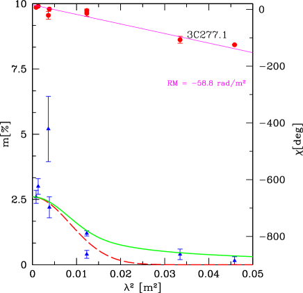
Figure 9: Position angles $\chi$ and fractional polarisation $m$ for the source 3C277.1. Layout as in Fig. 2.

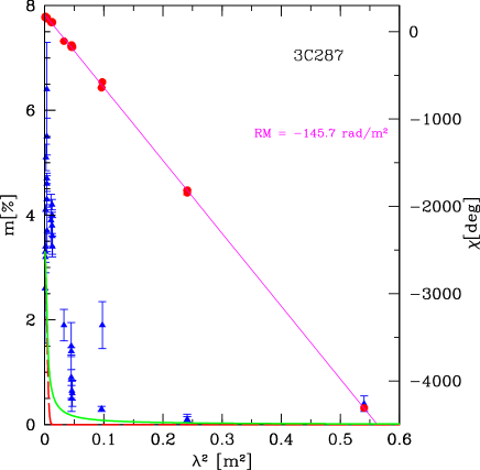
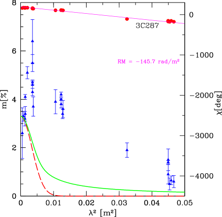
Figure 10: Position angles $\chi$ and fractional polarisation $m$ for the source 3C277.1. Layout as in Fig. 2.

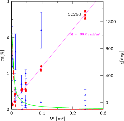
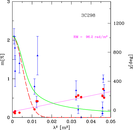
Figure 11: Position angles $\chi$ and fractional polarisation $m$ for the source 3C277.1. Layout as in Fig. 2.

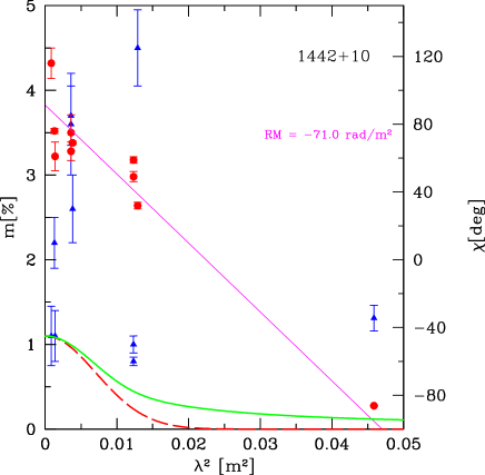
Figure 12: Position angles $\chi$ and fractional polarisation $m$ for the source 1442+10. Layout as in Fig. 2.

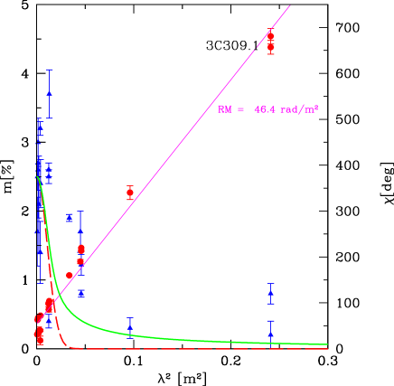
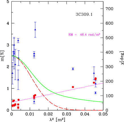
Figure 13: Position angles $\chi$ and fractional polarisation $m$ for the source 3C309.1. Layout as in Fig. 2.

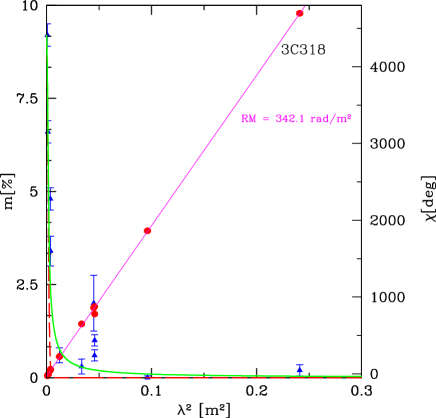
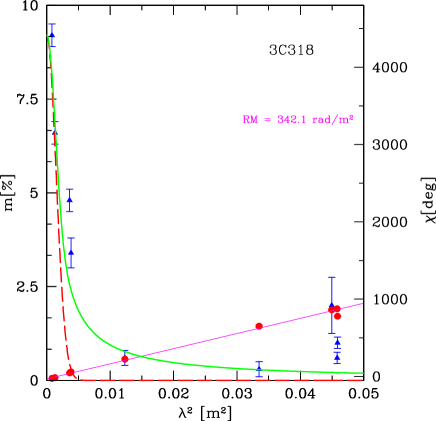
Figure 14: Position angles $\chi$ and fractional polarisation $m$ for the source 3C318. Layout as in Fig. 2.

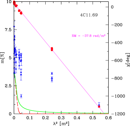
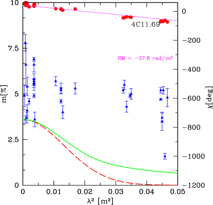
Figure 15: Position angles $\chi$ and fractional polarisation $m$ for the source 4C11.69. Layout as in Fig. 2.

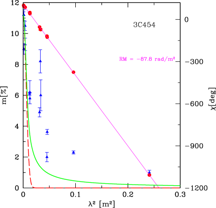
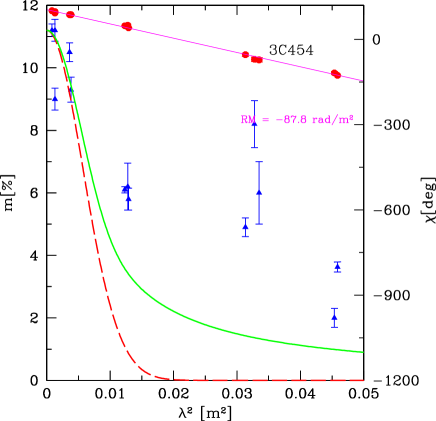
Figure 16: Position angles $\chi$ and fractional polarisation $m$ for the source 3C454. Layout as in Fig. 2.

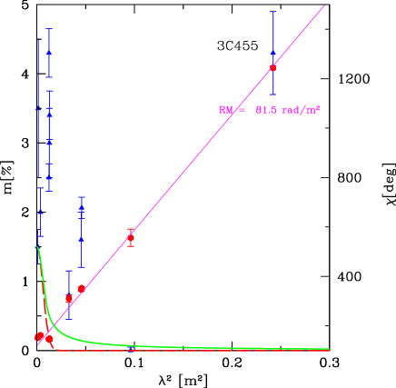
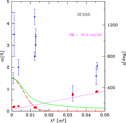
Figure 17: Position angles $\chi$ and fractional polarisation $m$ for the source 3C455. Layout as in Fig. 2.

Rotation Measures were calculated for about 1/3 of the sources in our list using use of our own measurements, NVSS and Tabara & Inoue data. The observed RMs were calculated for 16 sources with at least two measurements of the position angles achieved by Effelsberg and NVSS observations. Plots of the position angle of the electric vector in degrees versus the $\lambda^{2}$ in m² are shown in Figs. 2–17.

In all cases, the $\lambda^{2}$ law is closely followed for least squares estimates of the linear regression close to 1. To search for possible variability, we determined the RM both from our new measurements only and from all available measurements, including those of Tabara & Inoue, which were measured about 30 years ago. No significant difference was found.

The observing frequencies were suitably separated to enable an unambiguous rotation of the polarisation E-vectors. By analysing the combination of RM and fractional polarisation, we measured $\lambda^{2}$ rotation and depolarisation for all sources, which corresponded to depolarisation produced inside the source, and rotation produced outside. However, since $\delta\chi>\pi$, we actually observed not mixed-in gas but a foreground screen. A revised Tribble model such as that proposed by Rossetti et al. (2008) with a “partial coverage” of the source of radio emission by NLRs may account for the depolarisation behaviour.

Comments are necessary in a few cases.

- 3C67: the RM values calculated making use of the three position angles of Table 3 give an excellent least squares fit the by means of linear regression after rotating by both $+\rm and-\pi$ the nominal value of $59^{\circ}.3$ obtained at 1.4 GHz, namely 69 rad m^-2 and –71 rad m^-2. The last value is close to that ($-$67 rad m^-2) calculated also using the RMs listed in the Tabara & Inoue catalogue. 3C138: the RM value calculated with the position angles listed in Table 3 is –1 rad m^-2 with a very poor mean least squares fit.

- 3C286: the RM value is not given as the position angle of the electric vector (33^∘) for this source is taken as a reference to calibrate the position angles at all the observing frequencies.

- 3C455: the least squares fit obtained with the values of Table 3 is worse than that achieved using all the available data.

In conclusion, we adopt in all cases the RMs listed in Col. 11 of Table 4 calculated using the present measurements of the position angles plus those taken from the catalogue by Tabara & Inoue. The RMs in the source rest frames range between –20 rad m^-2 for 3C138 and $\sim$3900 rad m^-2 for 3C119. Seven sources have a RM $>$400 rad m^-2.

Examples of CSS sources with high values of $\mid$RM$\mid$ ($\geq$ 1000 rad m^-2 in the source rest frame) have been found in the past (O’Dea 1998 and references therein).

Three of them are in our list with measured integrated RMs, namely 3C119, 1442+101 and 3C318 for which we measured 3900 rad m^-2, –1450 rad m^-2, and 2260 rad m^-2 respectively. For the source 1442+101 (OQ172), observed by Udomprasert (1998) with the VLBA, RMs up to 22400 rad m^-2 were found. For 3C119, Kato et al. (1987) found 3400 rad m^-2 using single dish measurements. For 3C318, Taylor et al. (1992) determined a RM of 1400 rad m^-2 using VLA observations. There are however CSS sources in our sample with smaller values of RM.

As described in more detail in Appendix 2, the source 3C298 shows evidence of temporal variability in the fractional polarisation.

4.3 The “Cotton Effect”

As an example, we show the percentage of polarised emission versus the source’s linear size in kpc at a frequency of 8.35 GHz in Fig. 1. Linear dimensions for sources labelled with “*” in Table 4, for which $z$ became available after 1990, were calculated. We note that in the plot sources with linear sizes greater than 15 kpc are omitted and sources with polarised emission below the detection limits are plotted assuming $m=0$.

The most unexpected result that we find is the distribution of points drawn in the plots at the Effelsberg and the NVSS observing frequencies. Polarised sources are distributed all over the $m$ – $LS$ space. This seems to clash with the findings of Cotton et al. (2003) and Fanti et al. (2004) for the B3-VLA sample of CSS sources. Cotton et al. (2003) making use of NVSS at 1.4 GHz found that sources smaller than 6 kpc are weakly polarised, and that polarised sources have linear sizes greater than 6 kpc (“Cotton effect”). Both the jet and the counter-jet are included in the source linear size. This implies a drastic change in the interstellar medium at about 3 kpc. This result was later confirmed by Fanti et al. (2004), who observed the same sample with the VLA at 4.9 GHz and 8.5 GHz and with the WSRT at 2.64 GHz (Rossetti et al. 2008).

The main difference between the two samples, i.e., the B3-VLA and the present 3CR&PW sample of CSS sources, is represented by the number of quasars, 5-10% and 49%, respectively. Excluding the quasars, we find that the Cotton effect is clearly evident again. However, we also note three outliers, the galaxies 3C93.1, 3C268.3, and 3C318. On the other hand, it has been found by Rossetti et al. (2008) that the Cotton effect is not obeyed by all sources. This indicates that the current depolarisation scenarios might not fully explain the observed behaviour. This is also further indication that CSS sources optically identified with quasars may represent a separate class of objects.

5 Conclusions

With the present observations of a complete sample of CSS sources at 4 different frequencies made with the Effelsberg 100-m radio telescope and from archived NVSS data, the following results have been reached:

a) It is confirmed that CSS sources are weakly polarised, low values of the median fractional polarisation being found. Where $m$ can be compared with those obtained by Klein et al. (2003) for the steep spectrum extended radio sources selected in the B3-VLA sample, larger values are found, which are 2.2% at 1.4 GHz, 3.7% at 2.64 GHz, 5.2% at 4.85 GHz, and 5.8% at 10.45 GHz. The more sensitive VLA observations at 1.4 GHz of the CSS sources in the 3CR&PW sample extracted from the NVSS also show a median value for the fractional polarisation of $\sim$1.6%, which is rather low.

b) As expected, the percentage of polarised sources decreases from higher to lower frequencies. We found 22 sources polarised at 10.45 GHz, 16 sources polarised at 8.35 GHz, 10 sources polarised at both 4.85 GHz and 2.64 GHz, and 13 at 1.4 GHz. In general, the percentage of polarised emission remains almost constant down to 2.64 GHz, then drastically drops at frequencies below $\sim$2 GHz. There may be cases of repolarisation. Of particular interest, if this finding is confirmed, is the case of 3C455.

c) A case of variability with time of the fractional polarisation is suggested for the source 3C298.

d) The data obtained with these observations allowed us to determine the RMs for 16 sources. The RMs in the source rest frames range between –20 rad m^-2 for 3C138 and $\sim$3900 rad m^-2 for 3C119. Seven sources show a RM $>$400 rad m^-2, confirming the high values of the RM usually found for CSS sources.

e) In all cases the $\lambda^{2}$ law is followed closely. The observing frequencies were suitably separated to enable an unambiguous rotation of the polarisation E-vectors. Analysing the combination of RM and fractional polarisation, we identified $\lambda^{2}$ rotation and depolarisation for all sources. A revised Tribble model such as that proposed by Rossetti et al. (2008) with a “partial coverage” of the source of radio emission by NLRs may account for the depolarisation behaviour.

f) The $m$ - $LS$ diagram contains sources polarised at any linear size and at all available frequencies, including the NVSS 1.4 GHz data, i.e., also for sources smaller than 6 kpc in linear size, in contrast to the so-called “Cotton effect” later confirmed by Fanti et al. (2004) for the B3-VLA sample of CSS sources. However, plotting $m$ versus $LS$ for objects optically identified with galaxies, the so-called “Cotton effect” is reproduced. Discussing the interesting, large difference in the percentage of objects identified as quasars in the two samples was not a subject of the present investigation.

g) CSS sources optically identified with quasars may represent a separate class of objects.

Appendix 1

In this Appendix, we present plots of the fractional polarisation $m$ derived form our Effelsberg observations complemented with those extracted from the NVSS at 1.4 GHz and those taken from Tabara & Inoue (1980). The values of $m$ predicted by the models of Burn and Tribble are shown for comparison. Also plotted are polarisation angles versus $\lambda^{2}$ with their corresponding linear best fit.

Appendix 2

2.1 Sources following the Tribble model

The model proposed by Tribble reproduces the data of about one third of our sample, namely of 3C48, 3C67, 3C119, 3C138, 3C268.3, 3C277.1, and 3C318. Sources such as 3C48, 3C67, 3C138, and 3C277.1 also show RM$<\la$ few 10 rad m^-2, which is an indication of an unresolved foreground screen, presumably the halo of our own Galaxy.

The source 3C119, which has a very high RM and thus a fast decline in its fractional polarisation, might already be affected by significant depolarisation at wavelengths shorter than 2.8 cm. A higher m₀ would lead to depolarisation according to the Tribble law.

2.2 Sources with an indication of repolarisation

Eight sources (3C43, 0319+12, 3C287, 1442+10, 3C309.1, 4C11.69, 3C454, and 3C455) show indications of repolarisation, i.e., an increase in fractional polarisation with decreasing frequency, generally at short wavelengths $\la$10 cm; this corresponds to a relatively strong increase in fractional polarisation followed by a decline that can still be described by the Tribble law. This effect is visible despite possible instrumental effects of different telescopes and also considering that observations were made at different epochs. In three of these sources (3C309.1, 4C11.69, 3C454), the repolarisation effect is indeed confused with possible time variability. Focusing on our simultaneous measurements only, we still find constant or slightly increasing fractional polarisation with increasing wavelength, which is not predicted by any depolarisation model. In particular, the galaxy 3C455 shows a measured repolarisation greater than the 3$\sigma$ level between 10.45 GHz and 2.64 GHz together with a small value of the RM_rf (194 rad m^-2), which is an indication of the influence of a foreground screen, possibly an extended cloud with [OII] emission detected by Hes et al. (1996). A plausible mechanism would be the effect of shear layers caused by the interaction between the surface of an expanding source and the surrounding medium (Burn 1966).

The source 3C455 was observed with the VLA at 8.35 GHz by Bogers et al. (1994). It shows a triple structure with the indication of a jet joining the core with the south western lobe. The three components are almost aligned along the source major axis extending up to about 4$\arcsec$. However, 3C455 appears slightly resolved by the NVSS, which has a restoring beam of 45$\arcsec$, suggesting that the three components imaged by Bogers et al. are actually embedded in a more extended region of low brightness emission. This can be seen in the image available in the VLA Low-Frequency Sky Survey (VLSS; Cohen et al. 2007) at 74 MHz, which shows an even more extended structure of about 2$\arcmin$ in size. The existence of this extended emission is supported by the source spectral index, which indicates an upturn towards higher flux density above $\sim$100 MHz. Therefore, a second possible interpretation is that by observing at 2.64 GHz or lower frequencies, we have integrated the flux density and polarised flux density from that region. At 10.45 GHz, the steep spectrum extended structure is below the detection limit.

A similar case of repolarisation at a lower frequency was pointed out by Montenegro-Montes et al. (2008) for the source 1159+01.

2.3 Polarisation variability

Finally, 3C298 could exhibit time variability in its fractional polarisation. Unfortunately, the current data base does not provide a sufficient number of simultaneous measurements to prove this effect, which was reported for example by Aller et al. (2003) for the source 3C147.