Intermittency route to chaos for the nuclear billiard - a qualitative study

Abstract

We analyze on a simple classical billiard system the onset of chaotical behaviour in different dynamical states. A classical version of the ”nuclear billiard” with a $2D$ deep Woods-Saxon potential is used. We take into account the coupling between the single-particle and the collective degrees of freedom in the presence of dissipation for several vibrational multipolarities. For the considered oscillation modes an increasing divergence of the nucleonic trajectories from the adiabatic to the resonance regime was observed. Also, a peculiar case of intermittency is reached in the vicinity of the resonance, for the monopole case. We examine the order-to-chaos transition by performing several types of qualitative analysis including sensitive dependence on the initial conditions, single-particle phase space maps, fractal dimensions of Poincare maps and autocorrelation functions.

I Introduction

Deterministic chaos, is usually defined as irregular, unpredictable behaviour of the trajectories generated by nonlinear systems whose dynamical laws, involving no randomness or probabilities, predict a unique time evolution of a given system.

Over the last two decades an increasing number of papers have treated the study of the deterministic chaotical behaviour of Fermi nuclear systems burgio-95 ; baldo-96 ; baldo-98 ; blocki-78 ; ring-80 ; speth-81 ; wong-82 ; grassberger-83 ; sieber-89 ; rapisarda-91 ; abul-magd-91 ; blocki-92 ; blumel-92 ; baldo-93 ; blocki-93 ; berry-93 ; ott-93 ; bauer-94 ; hilborn-94 ; blumel-94 ; drozdz-94 ; drozdz-95 ; bauer1-95 ; jarzynski-95 ; bulgac-95 ; atalmi-96a ; atalmi-96b . The interest for analyzing the order-to-chaos transitions on such systems was linked to the problem of the onset of dissipation of collective systems through mainly one-body and two-body processes. Among these we mention the interaction of the nucleons with the potential well, the evaporation of individual nucleons in nuclear peripheral interactions, and the collisions between nucleons without taking into account the Pauli blocking effect.

These kinds of analyses were performed for the first time by Burgio, Baldo et al. burgio-95 ; baldo-96 ; baldo-98 considering a system of nucleons which move within a container modelled as a Woods-Saxon type potential and kick the container walls with a specific frequency. They discuss the damping of the movement and the relation with order-chaos transition in single-particle dynamics.

On that classical model worked Papachristou and collab. papachristou-08 , studying the decay width of the Isoscalar Giant Monopole Resonance for various spherical nuclei. Following also that formalism, the beginning of the chaotic behaviour for a number of nucleons in various dynamical regions at several multipolarities was surveyed felea-01 ; felea-02 ; bordeianu-08a ; bordeianu-08b ; bordeianu-08c .

In this paper, we investigated the chaotic behaviour of a single-nucleon in a two-dimensional ($2D$) deep Woods-Saxon potential well for specific physical phases. A qualitative picture of the achievement of deterministic chaos was shown for a comparative study between the adiabatic and the resonance stage of the nuclear interaction.

Close to resonance we obtained characteristics of the intermittency regime, i.e. sudden change to a laminar behaviour (so-called intermission) of a specific signal between two turbulent phases, which has been detected over and over again in a plethora of experiments regarding the Rayleigh-Benard convection, the driven nonlinear semiconductor oscillator, the Belousov-Zhabotinskii chemical reaction, and the Josephson junctions (for e.g., berge-80 ; pomeau-81 ; linsay-81 ; testa-82 ; jeffries-82 ; dubois-83 ; yeh-83 ; huang-87 ; richetti-87 ; kreisberg-91 ).

Albeit intermittency is a well-known phenomenon for billiards dahlqvist-92 ; dahlqvist-95 ; artuso-96 ; altmann-07 , in particular for Hamiltonian systems with divided phase space (e.g., mushroom bunimovich-01 ; bunimovich-03 ; altmann-05 ; altmann-06 ; porter-06 and annular billiards saito-82 ), and for connected Hamiltonian systems markus-03 , we showed that this property also holds for a Woods-Saxon billiard container with inelastic particle-wall interactions.

II Basic formalism

We chose for the present analysis a simple dynamical system as considered in several previous papers by Burgio and collab. burgio-95 ; baldo-96 ; baldo-98 . This system contains a number of $A$ spinless and chargeless nucleons, with no internal structure. The nucleons move in a $2D$ deep Woods-Saxon potential well considered as a ”nuclear billiard” and hit periodically the oscillating surface of the well with a certain frequency. The Bohr Hamiltonian of such a system in polar coordinates is considered as:

$$H\left(r_{j},\theta_{j},\alpha\right) = {\sum_{j=1}^{A}}\left[\frac{p_{r_{j}}^{2}}{2m}+\frac{p_{\theta_{j}}^{2}}{2mr_{j}^{2}}+V\left(r_{j},R\left(\theta_{j}\right)\right)\right]$$ (1)

$$+\frac{p_{\alpha}^{2}}{2M}+\frac{M\Omega^{2}\alpha^{2}}{2},$$

where $\left\{p_{r_{j}},p_{\theta_{j}},p_{\alpha}\right\}$ are the conjugate momenta of the particle and collective coordinates $\left\{r_{j},\theta_{j},\alpha\right\}$, the nucleon mass $m$ is $938\ \rm{MeV}$, $\Omega$ is the oscillating frequency of the collective variable $\alpha$, and $M=mAR_{0}^{2}$ is the Inglis mass.

The Woods-Saxon potential is constant inside the billiard and a very steeply rising function on the surface:

$$V\left(r_{j},R\left(\theta_{j}\right)\right)=\frac{V_{0}}{1+\exp\left[\frac{r_{j}-R\left(\theta_{j},\alpha\right)}{a}\right]},$$ (2)

with $V_{0}=-1500\ \rm{MeV}$, deep enough to prevent the escape of the nucleons regarded as classical objects for the present analysis. For the same reason, the diffusivity coefficient $a$ has a very small value $0.01\ \rm{fm}$. The vibrating surface can be written as in burgio-95 ; baldo-96 ; baldo-98 , depending on the collective variable and Legendre polynomials $P_{L}\left(\cos\theta_{j}\right)$:

$$R_{j}=R\left(\theta_{j},\alpha\right)=R_{0}\left[1+\alpha P_{L}\left(\cos\theta_{j}\right)\right],$$ (3)

where $R_{0}=6\ \rm{fm}$, and $L$ the multipolarity vibration degree of the potential well is $0$ for the monopole, $1$ for the dipole, and $2$ for the quadrupole case.

Once the hamiltonian is chosen, the numerical simulations are based on the solution of the Hamilton equations:

$$\stackrel{{\scriptstyle\cdot}}{{r_{j}}} = \frac{p_{r_{j}}}{m},\ \stackrel{{\scriptstyle\cdot}}{{p_{r_{j}}}}=\frac{p_{\theta_{j}}^{2}}{mr_{j}^{3}}-\frac{\partial V}{\partial r_{j}},$$ (4)

$$\stackrel{{\scriptstyle\cdot}}{{\theta_{j}}} = \frac{p_{\theta_{j}}}{mr_{j}^{2}},\ \stackrel{{\scriptstyle\cdot}}{{p_{\theta_{j}}}}=-\frac{\partial V}{\partial R_{j}}\cdot\frac{\partial R_{j}}{\partial\theta_{j}},$$ (5)

$$\stackrel{{\scriptstyle\cdot}}{{\alpha}} = \frac{p_{\alpha}}{M},\ \stackrel{{\scriptstyle\cdot}}{{p_{\alpha}}}=-M\Omega^{2}\alpha-\sum_{j=1}^{A}\left(\frac{\partial V}{\partial R_{j}}\cdot\frac{\partial R_{j}}{\partial\alpha}\right).$$ (6)

The Hamilton equations were solved with a Runge-Kutta type algorithm (order 2-3) having an optimized step size and taking into account that the absolute error for each variable is less than $10^{-6}$. Total energy was verified to be conserved with high accuracy to a relative error level of $10^{-8}$.

The equilibrium deformation parameter $\stackrel{{\scriptstyle-}}{{\alpha}}$, which is the mean collective variable, can be calculated (for e.g., for $L=0$) by equating the mechanical pressure of the wall, $P_{wall}$:

$$P_{wall}=\frac{M\Omega^{2}}{2\pi R_{0}^{2}}\cdot\frac{\stackrel{{\scriptstyle-}}{{\alpha}}}{1+\stackrel{{\scriptstyle-}}{{\alpha}}}.$$ (7)

The pressure exerted by the particles is $P_{part}$, $\rho$ denotes the particle density, and $T$ is the apparent temperature of the system that equals the 2D kinetic energy, using the natural system of units ($\hbar=c=k_{B}=1$):

$$P_{part}=\rho T=\frac{AT}{\pi R_{0}^{2}\left(1+\stackrel{{\scriptstyle-}}{{\alpha}}\right)^{2}}.$$ (8)

Thus, one gets the equation for the equilibrium value of the collective coordinate in 2D, in the monopole case:

$$\stackrel{{\scriptstyle-}}{{\alpha}}\left(1+\stackrel{{\scriptstyle-}}{{\alpha}}\right)=\frac{2T}{mR_{0}^{2}\Omega^{2}}.$$ (9)

Then a small perturbation of this collective variable was considered $\alpha\left(t=0\ \rm{fm}/c\right)=\ \stackrel{{\scriptstyle-}}{{\alpha}}+0.15$ burgio-95 ; baldo-96 ; baldo-98 and the evolution of the physical system was thoroughly investigated.

III The qualitative analysis of the route to chaos

III.1 On the resonance condition

One can choose the wall oscillation taking place close to adiabatic conditions, imposing a wall frequency smaller than the single-particle one. Thus, the frequency of vibration $\Omega_{ad}$ was chosen less than $0.05\ c/\rm{fm}$, which corresponds to an oscillation period equal to:

$$\tau_{wall}=\frac{2\pi}{\Omega_{ad}}\!\geq\!125.66\ \rm{fm}/c.$$ (10)

By introducing the maximum particle speed:

$$v=\sqrt{\frac{2T}{m}},$$ (11)

and the parameters as in burgio-95 ; baldo-96 ; baldo-98 : $R_{0}=6\ \rm{fm}$ and $T=36\ \rm{MeV}$, one can obtain the value for the single-particle period:

$$\tau_{part}=\frac{2R_{0}}{v}\approx 43.33\ \rm{fm}/c.$$ (12)

In addition to burgio-95 ; baldo-96 ; baldo-98 we introduced a physical constraint to this elementary physical system and continued that type of analysis necessary for the study of a nonintegrable dynamical system. At the beginning we considered a physical situation and we chose instead a static vibrating ”nuclear billiard”, a projectile nucleus having the same properties, colliding with a target nucleus. It is well-known that the nuclear interaction, at incident energies ranging from MeV to GeV, can result in a multitude of processes from the nuclear evaporation to complete fragmentation or multifragmentation, according to the impact parameter.

It was shown in bauer2-95 ; felea-99 that during this kind of processes even for peripheral events an unnegligeable amount of energy is transferred by nucleon-nucleon scattering to the nucleons of the projectile and not only the transverse momentum distributions, but also the longitudinal momentum distributions as measured in the projectile fragmentation rest frame can reveal the centrality status of the interaction. It can also offer a hint on the apparent temperature of a Fermi gas of nucleons which was found to be felea-99 near the isotopic temperatures, i.e. several MeV pochodzalla-87 ; kunde-91 ; morrissey-94 ; serfling-98 .

It was therefore supposed that the target fragmentation can be associated with a resonance process. In order to obtain such behaviour, the wall frequency was gradually increased to the resonance frequency $\Omega_{res}=0.145\ c/\rm{fm}$. However, nuclear evaporation or plain breakup of a projectile nucleus can take place long before this regime is achieved by redistributing energy between the nucleons themselves and also between single-particle degrees of freedom and collective ones. Individual nucleons or clusters can thus have enough kinetic energy to escalade the wall barrier.

We should also emphasize that we can either have the case that can be put in correspondence with a nuclear collision process, i.e. the variation of the nucleonic frequency oscillation as the apparent temperature of the nucleons in the nuclei increases (Eqs. 11 and 12), maintaining the potential well vibration constant, or respectively, the inverse situation in which the period between two consecutive collisions of the nucleon with the self-consistent mean field is kept invariable, while modifying the oscillation modes of the nuclear surface. The latter regards our studied case and is the reversed physical case previously described. It was used because of the specific choice of the ”toy model” parameters described in burgio-95 ; baldo-96 ; baldo-98 .

But the most realistic evolution of the nucleons in a chosen potential can assume a simultaneous variation of both angular frequencies. The resonance condition of the coupled classical oscillators should remain however an important condition for a rapid appearance of a deterministic chaotical behaviour of the physical system in study at different time scales. A proper analysis of a system should provide the variation of the collision radian frequency of the nucleons inside the ”billiard” as the apparent temperature increases and the change in the vibrating potential period, supposing that the multipolarity increases when pumping energy in the ”nuclear reservoir” during interaction. We can for example use in simulations, for nuclei with a large number of nucleons, the Liquid Drop Model or the Collective Model, which predict a frequency of vibration as function of the multipolarity deformation degree:

$$\Omega_{L}=\sqrt{\frac{C_{L}}{B_{L}}},$$ (13)

with $C_{L}$ being the elasticity coefficient, and $B_{L}$ the mass coefficient for the oscillator of $L$ multipolarity.

We will briefly discuss on how the resonance condition might look like and for which particular case(s) it can be applied. By reverting to the set of differential nonlinear Hamilton equations and combining the last two of them (see Eq. 6), it emerged:

$$\stackrel{{\scriptstyle..}}{{\alpha}}+\Omega^{2}\alpha=-\frac{V_{0}R_{0}}{aM}\cdot\sum_{j=1}^{A}P_{L}\left(\cos\theta_{j}\right)\frac{e^{\frac{r_{j}-R_{j}}{a}}}{\left[1+e^{\frac{r_{j}-R_{j}}{a}}\right]^{2}}.$$ (14)

One can now compare the resulted equation with a harmonic oscillator system in the presence of dissipative processes (”damped oscillator”) and of a external harmonic driving force of $F_{0}$ amplitude:

$$\stackrel{{\scriptstyle..}}{{\alpha}}+\Gamma\stackrel{{\scriptstyle.}}{{\alpha}}+\Omega^{2}\alpha=-\frac{F_{0}R_{0}}{M}\cdot cos\>\omega t.$$ (15)

In a first approximation we can neglect the damping constant $\Gamma$, as noticed from the Figs. 1-4. Besides, dissipation will appear if only the collective coordinate $\alpha$ is averaged over a large number of events, for all multipolarities considered burgio-95 ; baldo-98 . For the uncoupled equations ($UCE$) case there is no damping either, as the solution of a homogeneous Eq. 14 is a purely harmonic one: $\alpha=\alpha_{0}\>cos\>\Omega t$.

Also, we remark that for the dipole collective oscillations: $P_{1}\left(\cos\theta_{j}\right)=cos\>\omega_{j}t$ and that, for a statistical ensemble of $A$ nucleons, the one-particle radian frequency can be approximated with a constant, $\omega_{j}\approx\omega$. For the Woods-Saxon potential energy: $V(t)=\sum_{j=1}^{A}V(r_{j},\theta_{j},\alpha)$, it can always be derived a conservative force $F_{0}$:

$$F_{0}\left(t\right)=-\sum_{j=1}^{A}\frac{\partial V\left(t\right)}{\partial r_{j}}=\frac{V_{0}}{a}\cdot\sum_{j=1}^{A}\frac{e^{\frac{r_{j}-R_{j}}{a}}}{\left[1+e^{\frac{r_{j}-R_{j}}{a}}\right]^{2}}.$$ (16)

A similarity between Eq. 14 and 15 was eventually obtained, because once shifting towards collectives of nucleons, the total force becomes a sum over a number of time dependent forces, each acting on a single nucleon. Therefore, the net force for a pack of nucleons tends to vary little with time: $F_{0}\neq F_{0}(t)$, and the tendency increases with $A$.

In conclusion, the resonance condition, as stated in Eq. 14, can be definitely used for the multi-particle couplings with a dipolar shape of the potential well. This was verified by studying the variance of the largest Lyapunov exponent and of the Kolmogorov-Sinai entropy with the radian frequency of wall oscillation on a ten-nucleons system bordeianu-08c . For the other multipole degrees taken into account, and as well, for the dipole oscillations coupled with a single-nucleon dynamics, the nonlinear character of the differential Equation 14 offers a somewhat intricate perspective over obtaining an analytical generalized resonance condition, and for the moment is left aside for further investigation.

As we confine the following analysis on the single-particle chaotical dynamics, the frequency matching of the coupled oscillators: $\omega_{part}=\Omega_{res}=0.145\ c/\rm{fm}$, will be generically designated as the resonance stage of the interaction.

III.2 Dependence on the initial conditions

In order to detect chaos in simple systems, several customary methods are used schuster-84 . The sensitive dependence on the initial conditions, the so-called ”Butterfly effect” is the first type of analysis presented in this article. For a given multipolarity degree we studied the time dependence of both, single-particle and collective variables, with small perturbations applied to a single parameter (for e.g., $\Delta r=0.01\ \rm{fm}$). This type of analysis is presented for four cases, ranging from $UCE$ to quadrupole deformations of the two-dimensional wall surface, and for the two physical regimes in study, adiabatic and of resonance, respectively (Figs. 1-4).

At a first glance, the time dependence of the collective degrees of freedom ”looks chaotic” for all considered situations with the exception of $\left(4+2\right)$ uncoupled nonlinear differential equations case (Fig. 1), as one would naturally expect. In this case, a periodical structure would definitely appear in sharp contrast with the quasi-periodicity shown for different multipole collective modes. Also, the time evolution of the single-particle variables is clearly chaotic in all cases where the strong coupling between the $\left(4+2\right)$ nonlinear differential equations describing the single-particle dynamics appears (Figs. 2-4).

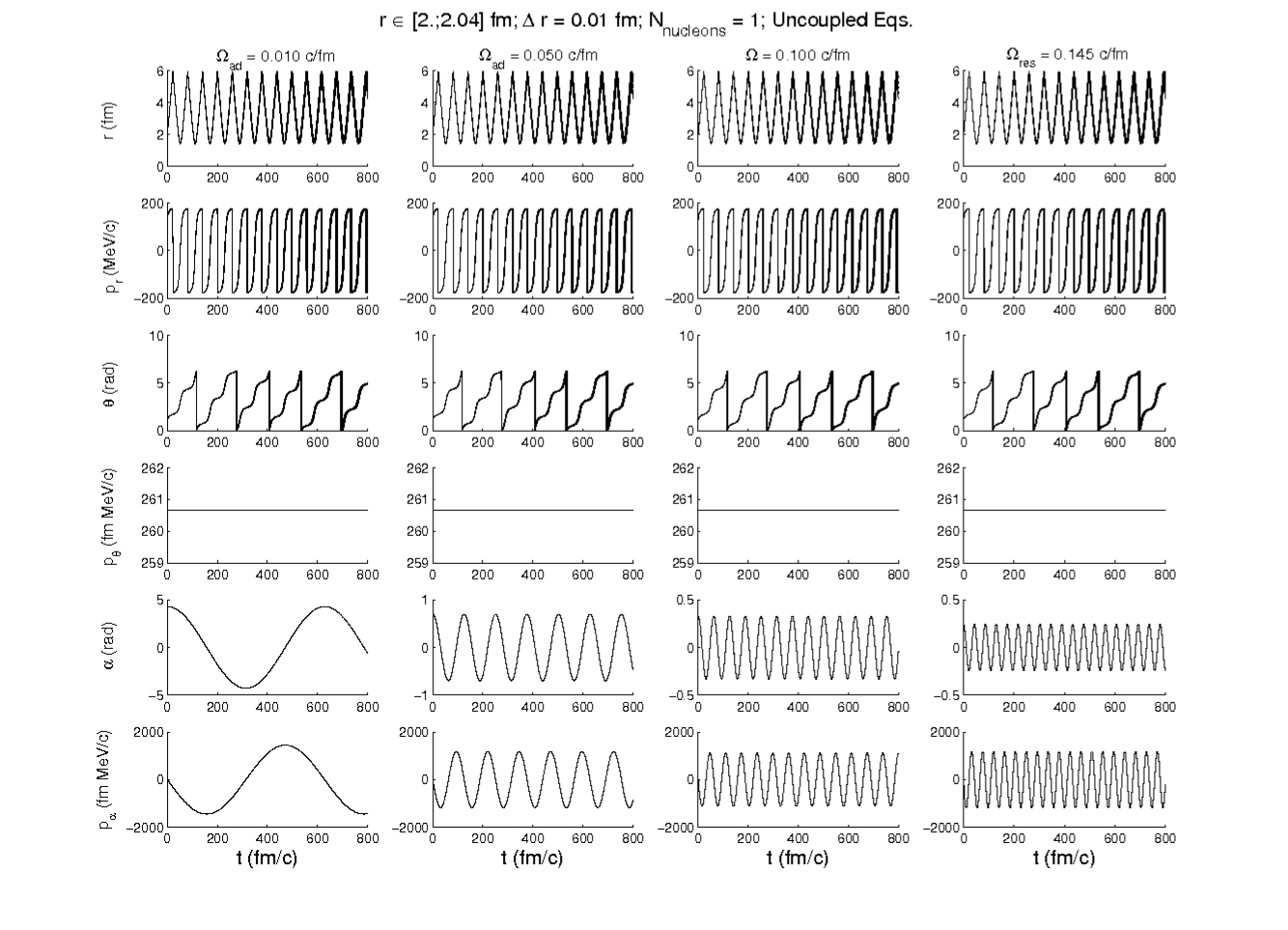
Figure 1: The sensitive dependence on the initial small perturbation of the radius parameter (0.01 fm/c) when adiabatic and resonance conditions are imposed (uncoupled one-nucleon and collective degrees of freedom case).

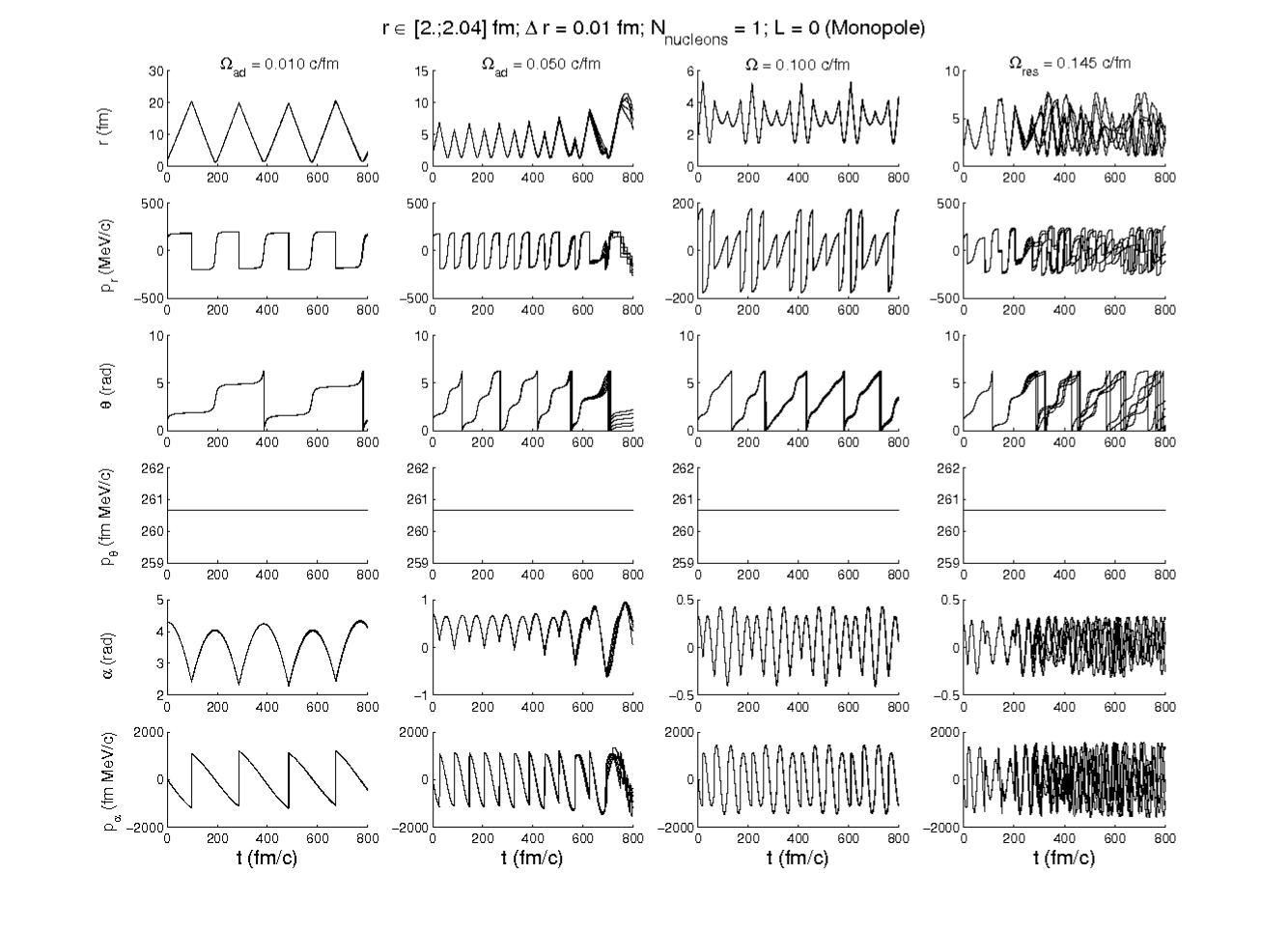
Figure 2: The sensitive dependence on the initial small perturbation of the radius parameter (0.01 fm/c) when adiabatic and resonance conditions are imposed (monopole case).

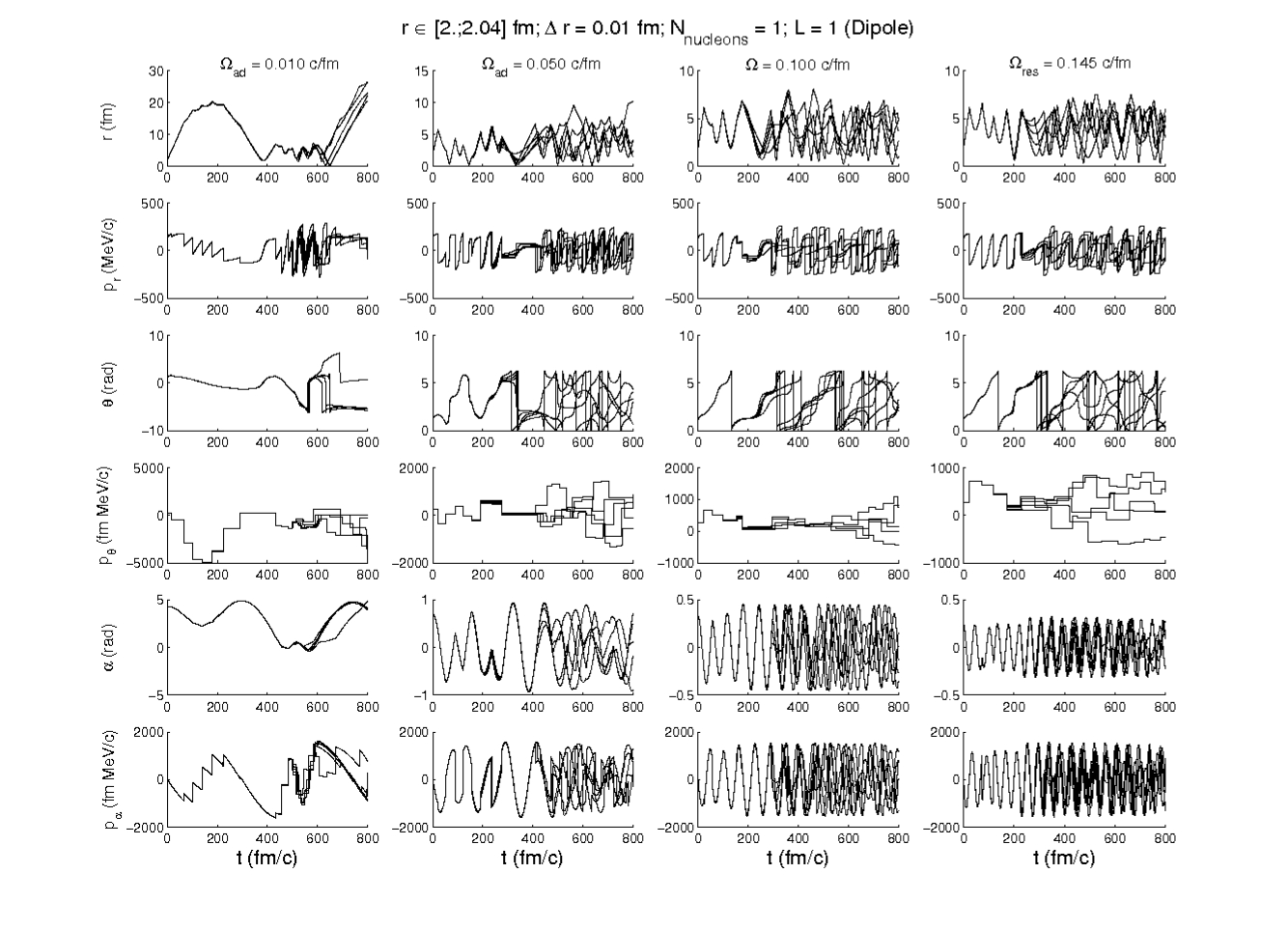
Figure 3: The sensitive dependence on the initial small perturbation of the radius parameter (0.01 fm/c) when adiabatic and resonance conditions are imposed (dipole case).

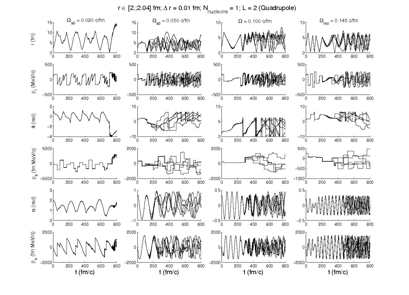
Figure 4: The sensitive dependence on the initial small perturbation of the radius parameter (0.01 fm/c) when adiabatic and resonance conditions are imposed (quadrupole case).

The sensitive dependence on the initial conditions, i.e. the decoupling of the trajectories at macroscopic scale, is found to give the first hints on the behaviour of the nuclear system, in its evolution from the quasi-stable states, which can hardly develop a chaotic motion in time (adiabatic state), to the unstable ones, characterized by a rapid divergence of the particle trajectories in the phase space (resonance regime). Also, in the monopole case the order-to-chaos transition clearly shows an intermittent pattern at $\Omega=0.1\ c/\rm{fm}$ (Fig. 2).

III.3 Maps of phase space

Another type of qualitative analysis, indicating different ways toward a chaotic behaviour is based on the one-dimensional maps of phase space.

Thus, for a temporal scale of $3,200\ \rm{fm}/c$ we represented the evolution of the multipolarity deformation degree of the potential well in the phase space of the vibrational variables $\left(\alpha\leftrightarrow p_{\alpha}\right)$, as well as in the $1D$ phase space of a single-particle $\left(r\leftrightarrow p_{r}\right)$. This type of analysis was performed for the $UCE$, monopole, dipole and quadrupole cases, using the same physical conditions, from the adiabatic to the resonance phase (Figs. 5-12).

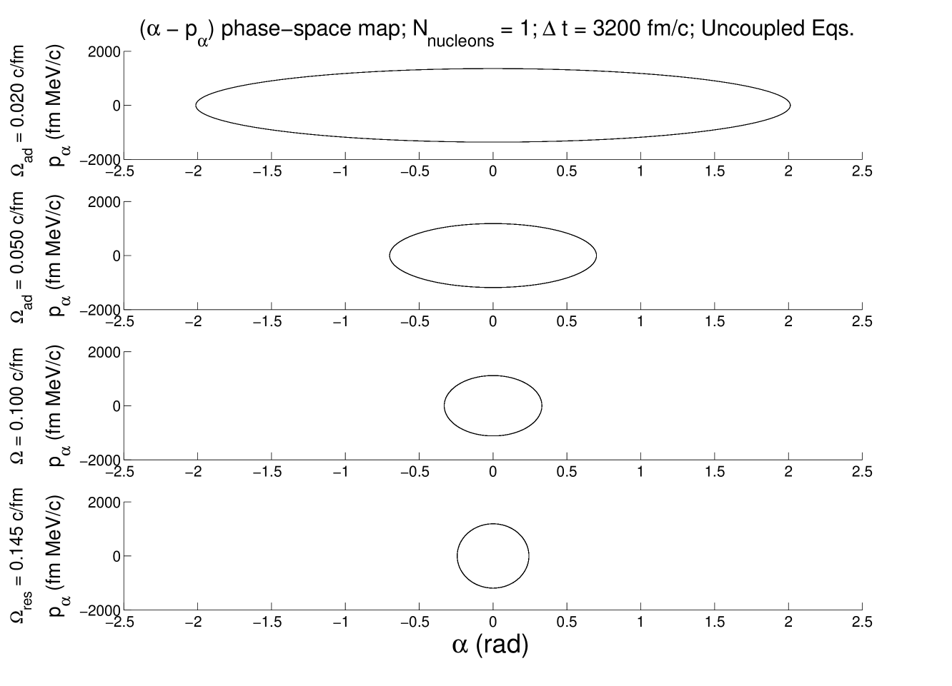
Figure 5: The phase space of the collective degrees of freedom ($\alpha-p_{\alpha}$) for different wall frequencies (uncoupled single and collective degrees of freedom case).

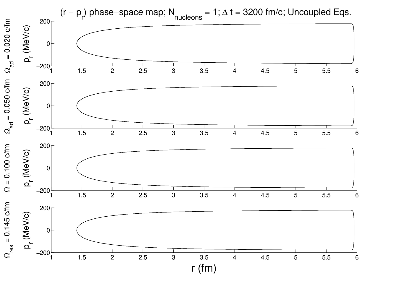
Figure 6: The phase space of the single-particle degrees of freedom ($r-p_{r}$) for different wall frequencies (uncoupled single and collective degrees of freedom case).

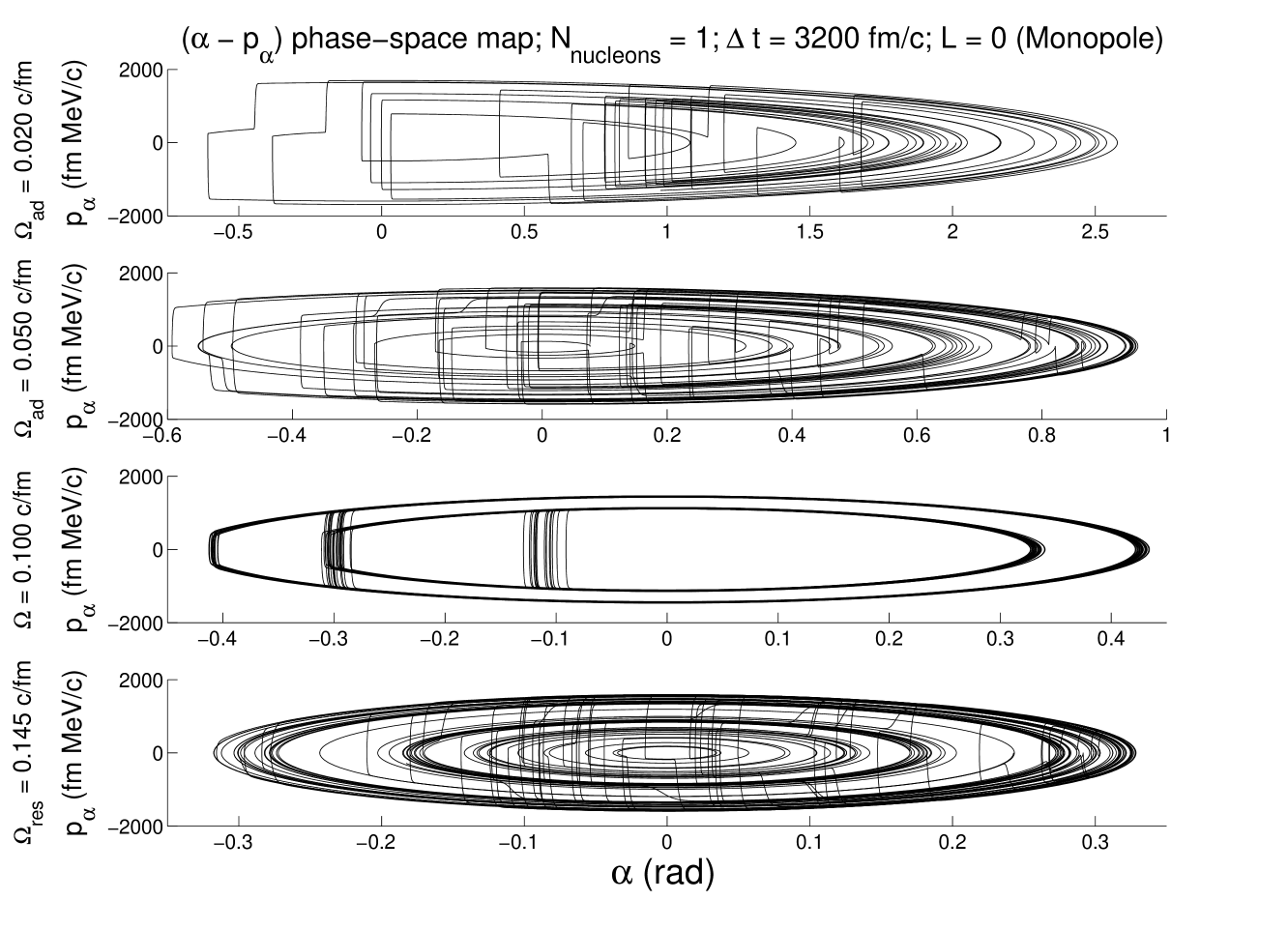
Figure 7: The phase space of the collective degrees of freedom ($\alpha-p_{\alpha}$) for different wall frequencies (L = 0).

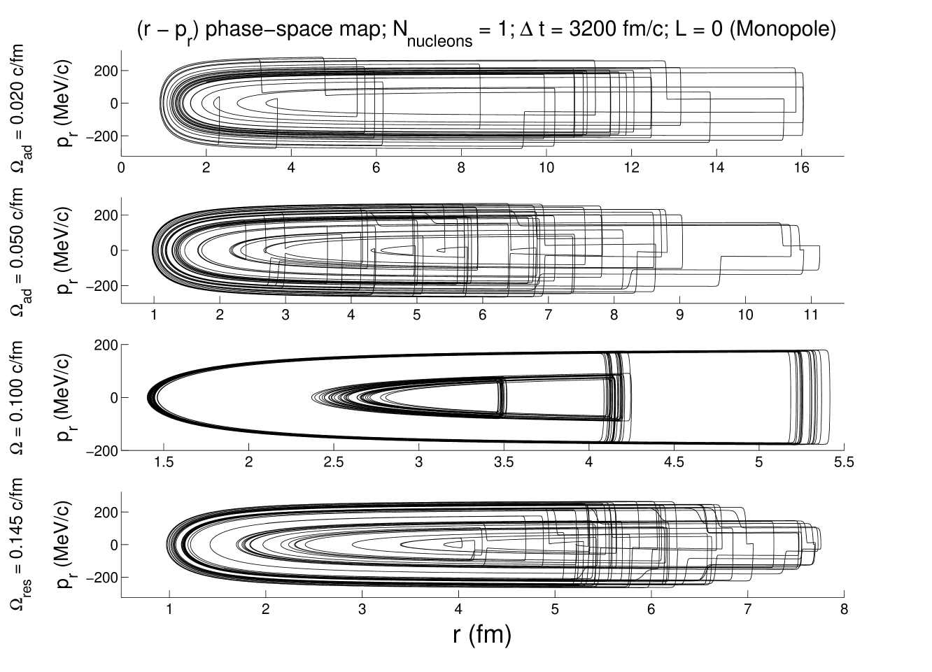
Figure 8: The phase space of the single-particle degrees of freedom ($r-p_{r}$) for different wall frequencies (L = 0).

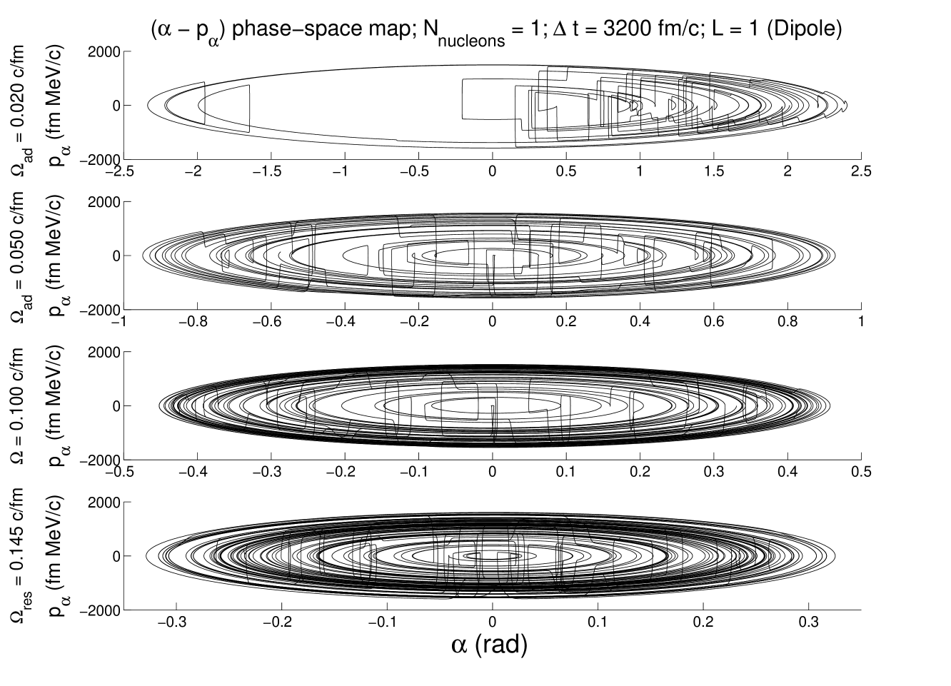
Figure 9: The phase space of the collective degrees of freedom ($\alpha-p_{\alpha}$) for different wall frequencies (L = 1).

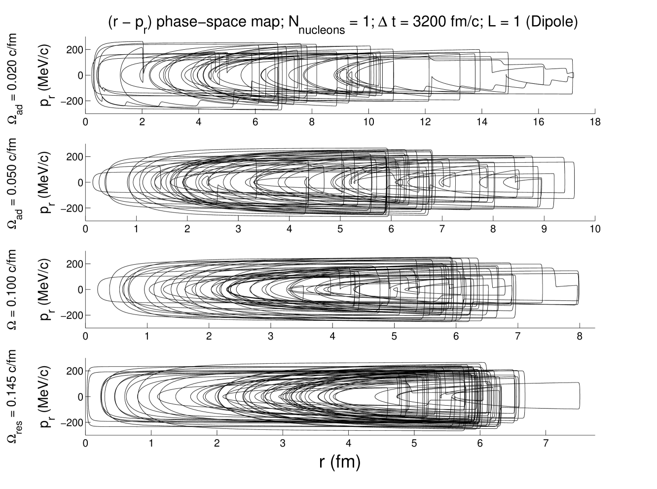
Figure 10: The phase space of the single-particle degrees of freedom ($r-p_{r}$) for different wall frequencies (L = 1).

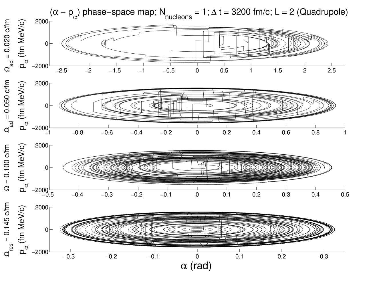
Figure 11: The phase space of the collective degrees of freedom ($\alpha-p_{\alpha}$) for different wall frequencies (L = 2).

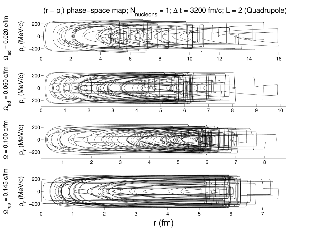
Figure 12: The phase space of the single-particle degrees of freedom ($r-p_{r}$) for different wall frequencies (L = 2).

A remark that can be formulated from the study of these phase space maps is related to the form of the trajectories specific to those described by a harmonic oscillator, especially for the $\left(\alpha\leftrightarrow p_{\alpha}\right)$ maps. It can be easily put to the test (Figs. 5, 7, 9, and 11) that the ellipse area $S_{h\!o}$ is proportionally inverse with the wall vibration frequency:

$$S_{h\!o}=\frac{2\pi\cdot E_{coll}}{\Omega},$$ (17)

where $E_{coll}$ is the sum of the last two terms from $(1)$, being the energy of the collective nucleonic motion.

The phase space filling degree raises as the vibration wall frequency moves towards the resonance value for all multipolarities took into account (Figs. 7-12), with the exception of the uncoupled nonlinear differential equations case (Figs. 5 and 6). This confirms that the characteristic time of the macroscopic decoupling of the nucleon trajectories in the Woods-Saxon potential evolves towards smaller values, once $\Omega$ is increased and also that the coupling between the collective variable motion and the particle dynamics is essential in amplifying the chaotic behaviour.

An intriguing aspect is revealed by the comparison of the filling degrees of the phase space as a function of the nucleon oscillation frequency in the chosen potential. One would expect that the trajectories degenerate from a simple orbit towards a compact filling of the $\left(\alpha\leftrightarrow p_{\alpha}\right)$ or $\left(r\leftrightarrow p_{r}\right)$ plane. Moreover, we observe several attraction basins around a few standard orbits, preeminently in the monopole case at $\Omega=0.1\ c/\rm{fm}$, characteristic feature of an intermittent behaviour (Figs. 7 and 8).

III.4 Fractal dimensions of Poincare maps

The one-dimensional phase space maps offer a hint on their filling degree in time. In the same manner one can use the Poincare maps for the ”nuclear billiard” regarded as a deterministic dynamical system. When analyzing the behaviour of close trajectories in the phase space, starting from a periodical orbit, Poincare showed poincare-890 ; poincare-892 that there are only three distinct possibilities: the curve can be either a closed one (with a fix distance to a periodical orbit), or it can be a spiral that asymptotically wraps/unfolds to/from the periodical trajectory.

In order to simplify the temporal analysis for peculiar orbits, Poincare suggested a simple and effective method. By choosing a transversal section with $\left(N-1\right)D$ that intersects a $ND$ geometrical variety, the sequence of the intersection points is easier to be studied than the whole $ND$ curve. Therefore, the cases previously described for the spiral generate a series of points that draw near in or move away from the intersection point of the periodical orbit with the transversal section.

Applying the Poincare maps type analysis to the simple chosen physical system, one would expect that the compact filling up of a $1D$ map of phase space for vibration frequencies of the Woods-Saxon well that match the one-particle oscillation frequencies inside the ”billiard” (Figs. 5-12), to reverberate by a large density of chaotic distributed intersection points.

In order to estimate the degree of fractality of such densities, we computed the fractal dimensions $d_{f}$ of the Poincare maps with one-nucleon radial degrees of freedom $\left(r\leftrightarrow p_{r}\right)$, when choosing for the transversal section the polar pair $\left(\theta\leftrightarrow p_{\theta}\right)$ as a constant. As only for the monopole and $UCE$ cases the orbital kinetic momentum is a constant of motion, we plotted the one-particle radius as a function of radial momentum when the polar coordinate is not kept constant, but quasi-constant in order to increase the probability of intersecting the section for a given time evolution of the system:

$$\theta=\theta_{0}\pm\epsilon_{\theta}.$$ (18)

We then chose a very small value for the $\left(\theta\leftrightarrow p_{\theta}\right)$ thickness: $\epsilon_{\theta}=10^{-4}$ radians and let the system evolve for a period of $\Delta t=5\cdot 10^{6}\ \rm{fm}/c$.

The values were calculated using the box counting algorithm in a specific Visual Basic 6 application grossu-09a ; grossu-09b on Poincare maps. The fractal dimension of a map covered by $N$ boxes of length $r$ is described by the following expression (see, for e.g., landau-07 ; landau-08 ):

$$d_{f}=\lim_{r\rightarrow 0}\frac{\log N\left(r\right)}{\log\left(1/r\right)},$$ (19)

where we took: $r=1/2^{n}$, $0\leq n\leq n_{max}$. The maximum value $n_{max}$ denotes the highest chosen resolution.

We calculated $d_{f}$ as slopes of the linear fits of $\log_{2}^{N\left(r\right)}$ versus $n=\log_{2}^{1/r}$ points, where we took the inferior limit of $log(1/r)$ to be $5$, and the superior threshold according to the highest resolutions for which a saturation plateau appears: $N\neq N(r)$ (Fig. 13). At resolutions above threshold, no additional information on the points distribution can be gained.

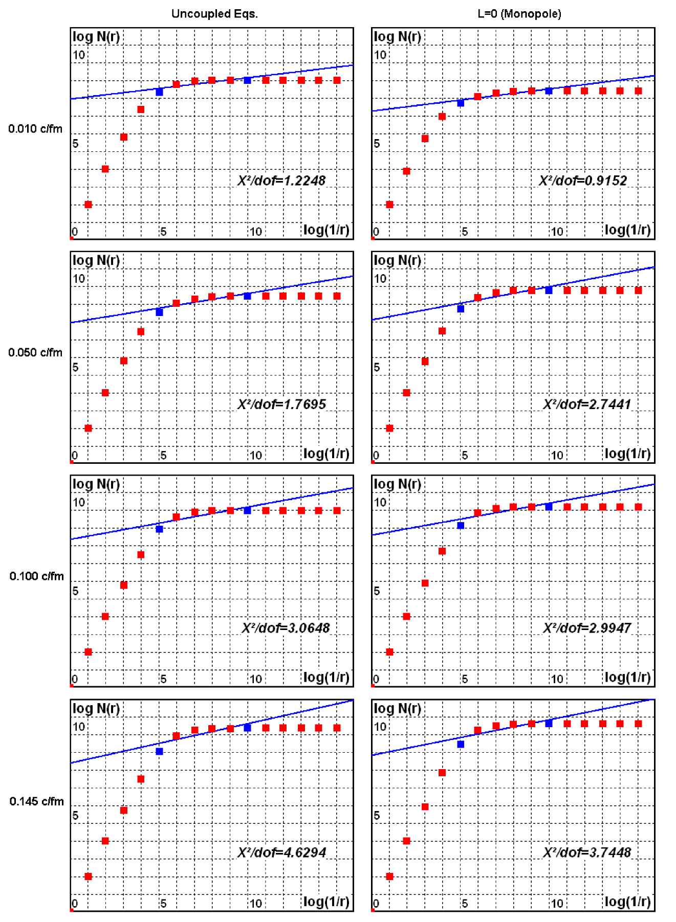
Figure 13: The fractal dimensions of the (radius $\leftrightarrow$ radial momentum) Poincare one-nucleon maps as linear slopes.

The points from the Poincare maps are distributed in such a way that up to a certain resolution ($32\times 32$ pixels) the algorithm does not take into account the individual pixels. In this first region analyzed the alignment is quite good, denoting a correlation between points. The information is not uniformly distributed in the phase space but represents a ”cloud” of points with $d_{f}$ greater than $1$. This large-scale region thus offers a global image of the Poincare maps.

Above $32\times 32$ resolution appear the effects linked with the contribution of the individual dots of the Poincare maps, reflected by significant variations of the fractal dimensions. By choosing the points for the fitting procedure in such a way, we are also in agreement with the following criterion: the fitted points should be singled out so their associated resolutions are to be pertained to at least three successive decimal logarithmic intervals mandelbrot-82 . In Figure 13 we selected two points with resolutions belonging to the first interval $\left[10\div 10^{2}\right]$, three points to $\left[10^{2}\div 10^{3}\right]$, and we took one point in the $\left[10^{3}\div 10^{4}\right]$ range, just until constant values $N$ are reached.

The small-scale $d_{f}$ thus computed (Table 1) represent the filling degrees of a fine detailed phase space and can be correlated with the Shannon entropies calculated in felea-09b .

Table 1: The $d_{f}$ of the $\left(r\leftrightarrow p_{r}\right)$ Poincare single-particle maps

Oscillation frequency	Uncoupled eqs.	Monopole case
$\Omega\>_{ad}=0.010\>c/\rm{fm}$	$0.1194$	$0.1262$
$\Omega\>_{ad}=0.050\>c/\rm{fm}$	$0.1666$	$0.1870$
$\Omega\>\;\ \ =0.100\>c/\rm{fm}$	$0.1840$	$0.1790$
$\Omega_{res}=0.145\>c/\rm{fm}$	$0.2227$	$0.2010$

It can be remarked that the fractal dimensions generally increase with the specific vibration frequencies, from the quasi-stationary equilibrium regime at adiabatic oscillations to the unstable chaotical states of the nucleonic system in the resonance domain. At the same time, it should be mentioned that for the monopole case the fractal dimension has an intermittent deportment close to the resonance phase of interaction, at $\Omega=0.1\ c/\rm{fm}$.

III.5 Autocorrelation functions

The transition toward a quasi-periodical, aperiodical or chaotic behaviour can be also analyzed with the autocorrelation function of the variables characteristic for the temporal evolution of the studied physical system. When the ”nuclear billiard” evolves to chaos, essential changes can be noticed in the shape of the autocorrelation function of a specific variable (continuous or discrete distributed). This type of function measures the correlation between a sequence of signals, and is usually defined as:

$$C\left(\tau\right)=\lim_{T\rightarrow\infty}\frac{1}{T}\int^{T}_{0}\xi\left(t\right)\cdot\xi\left(t+\tau\right)\ dt;$$ (20)

$$\xi\left(t\right)=x\left(t\right)-\lim_{T\rightarrow\infty}\frac{1}{T}\int^{T}_{0}x\left(t\right)\ dt;$$ (21)

$$C\left(\tau\right)=\lim_{N\rightarrow\infty}\frac{1}{N}\sum^{N}_{n=0}\xi\left(t_{n}\right)\cdot\xi\left(t_{n+1}\right);$$ (22)

$$\xi\left(t_{n}\right)=x\left(t_{n}\right)-\lim_{N\rightarrow\infty}\frac{1}{N}\sum^{N}_{n=0}\xi\left(t_{n}\right).$$ (23)

For a laminar regular regime this function either has a constant value or presents decreasing oscillations in time. During a chaotic phase, it falls in, having an exponentially decreasing behaviour for uncorrelated signals, as shown in roux-81 .

We represented the autocorrelation function for the study of the single-particle (Fig. 14) and collective dynamics (Fig. 15). The analysis was thus done autocorrelating the radial momentum $p_{r}$ of the particle and respectively the collective variable $\alpha$ for the $UCE$ case and for all multipolarities, from all stages of interaction taken into account. One conclusion, that can be easily drawn from these figures, confirmed the previous results obtained with the other two methods. Thus, it can be noticed the increase of the chaotic bearing once the oscillation frequency of the potential well is varied from the adiabatic to the resonance regime, for all degrees of multipole.

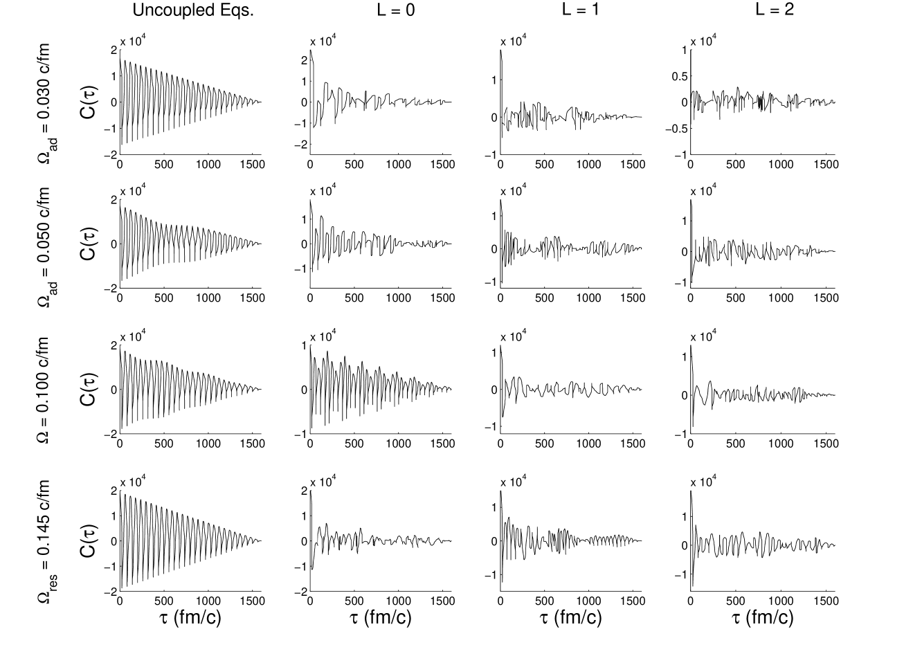
Figure 14: The autocorrelation function which correlates the radial momentum of a single-particle in time for various stages of nuclear interactions (from adiabatic to resonance regimes) and for several nuclear multipole deformations.

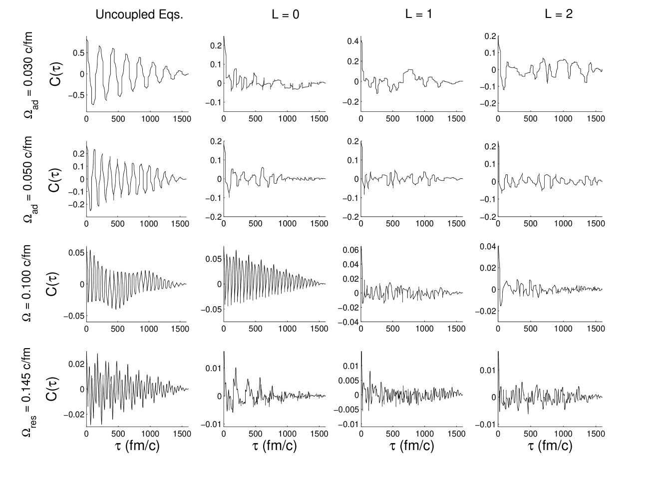
Figure 15: The autocorrelation function which correlates the collective variable in time for various stages of nuclear interactions (from adiabatic to resonance regimes) and for several nuclear multipole deformations.

When studying the case with single-particle degrees of freedom uncoupled from the collective ones, the dominant behaviour is aperiodical oscillation in time characteristic for a steady adiabatic phase of the interaction, even though the vibration frequency is varied. Only at resonance the shape is somewhat changed, indicating a greater degree of chaos.

As for the monopole to quadrupole deformations the decreasing of the autocorrelation function is indeed of the exponential type, steeper as the radian frequency of oscillation is raised to $\Omega_{res}=0.145\ c/\rm{fm}$.

The exception is again found in the monopole case at $\Omega=0.1\ c/\rm{fm}$ frequency of oscillation, when the intermittent phase of the interaction, reflected by aperiodical oscillations, points out a steady behaviour prior to the resonance regime.

IV Conclusions

A comparative study was done between the interesting physical regimes of nuclear interaction: adiabatic and resonance, giving at this level only a qualitative picture of the possible scenarios towards a pure deterministic behaviour of chaotic type of the studied nucleonic system.

We envisaged the single-nucleon dynamics in a Woods-Saxon potential. The coupling between individual and collective degrees of freedom was shown to generate different paths to chaos, according to the order of multipolarity. In general, for all vibrational modes at the resonance frequency of oscillation, the onset of chaotical behaviour was found to be earlier than at any other adiabatic vibrations of the 2D potential well.

Also, a phase alternation of periodical and chaotic dynamics was found in the monopole case of nuclear wall oscillation at $\Omega=0.1\ c/\rm{fm}$, revealing a laminar dynamics prior to the resonance stage of interaction.

In order to verify the aforementioned results, the study was completed with the inclusion of several quantitative analyses, inter alia we mention: power spectra, Shannon informational entropies, and Lyapunov exponents felea-09b .

- (1) G.F. Burgio, M. Baldo, A. Rapisarda, and P. Schuck, Phys. Rev. C 52, 2475 (1995).
- (2) M. Baldo, G.F. Burgio, A. Rapisarda, and P. Schuck, in Proceedings of the International Winter Meeting on Nuclear Physics, Bormio, Italy, 1996, edited by I. Iori. arXiv:nucl-th/9602030
- (3) M. Baldo, G.F. Burgio, A. Rapisarda, and P. Schuck, Phys. Rev. C 58, 2821 (1998).
- (4) J. Blocki, Y. Boneh, J.R. Nix, J. Randrup, M. Robel, A.J. Sierk, and W.J. Swiatecki, Ann. Phys. (N.Y.) 113, 330 (1978).
- (5) P. Ring and P. Schuck, The Nuclear Many Body Problem (Springer-Verlag, Berlin, 1980) p. 388.
- (6) J. Speth and A. van der Woude, Rep. Prog. Phys. 44, 719 (1981).
- (7) C.Y. Wong, Phys. Rev. C 25, 1460 (1982).
- (8) P. Grassberger and I. Procaccia, Phys. Rev. Lett. 50, 346 (1983).
- (9) M. Sieber and F. Steiner, Physica D 44, 248 (1990).
- (10) A. Rapisarda and M. Baldo, Phys. Rev. Lett. 66, 2581 (1991).
- (11) A.Y. Abul-Magd and H.A. Weidenmüller, Phys. Lett. B 261, 207 (1991).
- (12) J. Blocki, F. Brut, T. Srokowski, and W.J. Swiatecki, Nucl. Phys. A545, 511c (1992).
- (13) R. Blümel and J. Mehl, J. Stat. Phys. 68, 311 (1992).
- (14) M. Baldo, E.G. Lanza, and A. Rapisarda, Chaos 3, 691 (1993).
- (15) J. Blocki, J.J. Shi, and W.J. Swiatecki, Nucl. Phys. A554, 387 (1993).
- (16) M.V. Berry and J.M. Robbins, Proc. R. Soc., London, Sect. A 442, 641 (1993).
- (17) E. Ott, Chaos in Dynamical Systems (Cambridge University Press, Cambridge, England, 1993).
- (18) W. Bauer, D. McGrew, V. Zelevinsky, and P. Schuck, Phys. Rev. Lett. 72, 3771 (1994).
- (19) R. Hilborn, Chaos and Nonlinear Dynamics (Oxford University Press, Oxford, England, 1994).
- (20) R. Blümel and B. Esser, Phys. Rev. Lett. 72, 3658 (1994).
- (21) S. Drozdz, S. Nishizaki, and J. Wambach, Phys. Rev. Lett. 72, 2839 (1994).
- (22) S. Drozdz, S. Nishizaki, J. Wambach, and J. Speth, Phys. Rev. Lett. 74, 1075 (1995).
- (23) W. Bauer, D. McGrew, V. Zelevinsky, and P. Schuck, Nucl. Phys. A583, 93 (1995).
- (24) C. Jarzynski, Phys. Rev. Lett. 74, 2937 (1995).
- (25) A. Bulgac and D. Kusnezov, Chaos, Solitons and Fractals 5, 1051 (1995).
- (26) A. Atalmi, M. Baldo, G.F. Burgio, and A. Rapisarda, Phys. Rev. C 53, 2556 (1996). arXiv:nucl-th/9509020
- (27) A. Atalmi, M. Baldo, G.F. Burgio, and A. Rapisarda, in Proceedings of the International Winter Meeting on Nuclear Physics, Bormio, Italy, 1996, edited by I. Iori. arXiv:nucl-th/9602039
- (28) P.K. Papachristou, E. Mavrommatis, V. Constantoudis, F.K. Diakonos, and J. Wambach, Phys. Rev. C 77, 044305 (2008). arXiv:nucl-th/0803.3336
- (29) D. Felea, C. Beşliu, R.I. Nanciu, Al. Jipa, I.S. Zgură, R. Mărginean, M. Haiduc, A. Gheaţă, and M. Gheaţă, in Proceedings of the International Conference ”Nucleus-Nucleus Collisions”, Strasbourg, 2000, edited by W. Norenberg et al. (North-Holland, Amsterdam, The Netherlands, 2001) p. 222.
- (30) D. Felea, The Study of Nuclear Fragmentation Process in Nucleus-Nucleus Collisions at Energies higher than 1 A GeV, Ph.D. thesis, University of Bucharest, Faculty of Physics (2002) p. 134.
- (31) C.C. Bordeianu, C. Beşliu, Al. Jipa, D. Felea, and I.V. Grossu, Comput. Phys. Commun. 178, 788 (2008).
- (32) C.C. Bordeianu, D. Felea, C. Beşliu, Al. Jipa, and I.V. Grossu, Comput. Phys. Commun. 179, 199 (2008).
- (33) C.C. Bordeianu, D. Felea, C. Beşliu, Al. Jipa, and I.V. Grossu, Rom. Rep. in Phys. 60, 287 (2008).
- (34) Y. Pomeau and P. Manneville, Commun. Math. Phys. 74, 189 (1980).
- (35) P. Berge, M. Dubois, P. Manneville, and Y. Pomeau, J. Phys. (Paris) 41, L344 (1980).
- (36) Y. Pomeau, J.C. Roux, A. Rossi, S. Bachelart, and C. Vidal, J. Phys. (Paris) 42, L271 (1981).
- (37) P.S. Linsay, Phys. Rev. Lett. 47, 1349 (1981).
- (38) J. Testa, J. Perez, and C. Jeffries, Phys. Rev. Lett. 48, 714 (1982).
- (39) C. Jeffries and J. Perez, Phys. Rev. A 26, 2117 (1982).
- (40) M. Dubois, M.A. Rubio, and P. Berge, Phys. Rev. Lett. 51, 1446 (1983).
- (41) W.J. Yeh and Y.H. Kao, Appl. Phys. Lett. 42, 299 (1983).
- (42) J.Y. Huang and J.J. Kim, Phys. Rev. A 36, 1495 (1987).
- (43) P. Richetti, P. DeKepper, J.C. Roux, and H.L. Swinney, J. Stat. Phys. 48, 977 (1987).
- (44) N. Kreisberg, W.D. McCormick, and H.L. Swinney, Physica D 50, 463 (1991).
- (45) P. Dahlqvist, J. Phys. A 25, 6265 (1992).
- (46) P. Dahlqvist, Nonlinearity 8, 11 (1995).
- (47) R. Artuso, G. Casati, and I. Guarneri, J. Stat. Phys. 83, 977 (1996).
- (48) E.G. Altmann, Intermittent Chaos in Hamiltonian Dynamical Systems, Ph.D. thesis, Max Planck Institute for the Physics of Complex Systems in Dresden (2007), WUB-DIS 2007-02.
- (49) L.A. Bunimovich, Chaos 11, 802 (2001).
- (50) L.A. Bunimovich, Chaos 13, 903 (2003).
- (51) E.G. Altmann, A.E. Motter, and H. Kantz, Chaos 15, 033105 (2005). arXiv:nlin/0502058v2
- (52) E.G. Altmann, A.E. Motter, and H. Kantz, Phys. Rev. E 73, 026207 (2006). arXiv:nlin/0601008v1
- (53) M.A. Porter and S. Lansel, Notices of the AMS 53, 334 (2006).
- (54) N. Sait, H. Hirooka, J. Ford, F. Vivaldi, and G.H. Walker, Physica D 5, 273 (1982).
- (55) M. Markus and M. Schmick, Physica A 328, 335 (2003).
- (56) W. Bauer, Phys. Rev. C 51, 803 (1995).
- (57) C. Beşliu, D. Felea, V. Topor-Pop, A. Gheaţă, I.S. Zgură, Al. Jipa, and R. Zaharia, Phys. Rev. C 60, 024609 (1999).
- (58) J. Pochodzalla et al., Phys. Rev. C 35, 1695 (1987).
- (59) G.J. Kunde et al., Phys. Lett. B 272, 202 (1991).
- (60) D.J. Morrissey, W. Benenson, and W.A. Friedman, Annu. Rev. Nucl. Part. Sci. 44, 27 (1994).
- (61) V. Serfling et al., Phys. Rev. Lett. 80, 3928 (1998).
- (62) H.G. Schuster, Deterministic Chaos: an introduction (Physik-Verlag, Weinheim, Federal Republic of Germany, 1984).
- (63) H.J. Poincare, Acta Math. 13, (1890).
- (64) H.J. Poincare, Les Methodes Nouvelles de la Mechanique Celeste (Gauthier-Villars, Paris, 1892); English version: N.A.S.A. Translation TT F-450/452 (U.S. Fed. Clearinghouse, Springfield, VA, U.S.A., 1967).
- (65) I.V. Grossu, C. Beşliu, M.V. Rusu, Al. Jipa, C.C. Bordeianu, and D. Felea, Comput. Phys. Commun. 180, 1999 (2009). arXiv:0901.4643
- (66) I.V. Grossu, D. Felea, C. Beşliu, Al. Jipa, C.C. Bordeianu, E. Stan, and T. Eşanu, Comput. Phys. Commun., DOI: 10.1016/j.cpc.2009.12.005 (in press).
- (67) R.H. Landau, M.J. Pez, and C.C. Bordeianu, Computational Physics - Problem Solving with Computers (WILEY-VCH Verlag GmbH Et Co. KGaA, Weinheim, Germany, 2007) p. 304.
- (68) R.H. Landau, M.J. Pez, and C.C. Bordeianu, A Survey of Computational Physics - Introductory Computational Science (Princeton University Press, Princeton, New Jersey, USA, and Woodstock, Oxfordshire, UK, 2008) p. 335.
- (69) B.B. Mandelbrot, The Fractal Geometry of Nature (W.H. Freeman and Co., San Francisco, CA, U.S.A., 1982). Revised edition of Fractals: Form, Chance and Dimension (W.H. Freeman and Co., San Francisco, CA, U.S.A., 1977).
- (70) D. Felea, C.C. Bordeianu, I.V. Grossu, C. Beşliu, Al. Jipa, A.A. Radu, and E. Stan, ”Intermittency route to chaos for the nuclear billiard - a quantitative study”, Phys. Rev. C (submitted).
- (71) J.C. Roux, A. Rossi, S. Bachelart, and C. Vidal, Physica D 2, 395 (1981).