Total number of pages: 31

Number of tables: 2

Number of figures: 7

ABSTRACT

Shear and bulk viscosity and thermal conductivity for argon, krypton, xenon, and methane and the binary mixtures argon+krypton and argon+methane were determined by equilibrium molecular dynamics with the Green-Kubo method. The fluids were modeled by spherical Lennard-Jones pair-potentials with parameters adjusted to experimental vapor liquid-equilibria data alone. Good agreement between the predictions from simulation and experimental data is found for shear viscosity and thermal conductivity of the pure fluids and binary mixtures. The simulation results for the bulk viscosity show only poor agreement with experimental data for most fluids, despite good agreement with other simulations data from the literature. This indicates that presently available experimental data for the bulk viscosity, a property which is difficult to measure, are inaccurate.

KEYWORDS: Viscosity; Thermal conductivity; Green-Kubo; Lennard-Jones; Molecular Dynamics; Molecular Simulation.

1. Introduction

Transport properties play an important role in many technical and natural processes. With the rapid increase of available computing power, molecular simulation in combination with molecular modeling is becoming an interesting option for describing transport properties in regions where experimental data are not available or difficult to obtain. The calculation of transport coefficients by molecular simulation can be achieved by non-equilibrium molecular dynamics (NEMD) or equilibrium molecular dynamics (EMD). In NEMD, transport coefficients are calculated as the ratio of a flux to an appropriate driving force, extrapolating to the limit of zero driving force [1]. In EMD transport coefficients are often calculated by the Green-Kubo formalism [2, 3]. The choice between EMD and NEMD is largely a matter of taste and inclination, see e.g. [4, 5, 6]. There are numerous contributions in the literature in which both methods were applied for the calculation of shear viscosity [4, 7, 8, 10, 11, 12], bulk viscosity [13, 14, 15], and thermal conductivity [7, 10, 11, 16, 17] with comparable performance. To our knowledge the most comprehensive study on transport coefficients of the spherical Lennard-Jones fluid is reported in [18, 19]. Despite of the large number of publications on simulation of transport properties with the spherical Lennard-Jones potential, not much effort seems to have been spent on a comparison of simulation results with experimental data of real fluids. Exceptions are the works of Michels et al. [20] and Heyes et al. [10, 11]. Michels et al. [20] compared the self-diffusion coefficient to the Chapman-Enskog theory and experimental data for krypton and methane at high densities, but thermodynamic properties were not considered. Heyes et al. [10, 11] simulated both transport and thermodynamic properties of argon+krypton, argon+methane, and methane+nitrogen, but properties of pure fluids were not considered. In other cases [21, 22] more complex molecules like ethylene, carbon dioxide, phenol, alkanes, or carbon tetrachloride were modeled by the spherical Lennard-Jones potential, which surely is an oversimplification. Simulation data on transport properties were compared there to experimental data, but not the thermodynamic properties.

The interest here lies in the quantitative evaluation of the performance of Lennard-Jones models [23], which have been optimized for the accurate prediction of thermodynamic properties, in the description of transport properties. In this work EMD is used to carry out a comprehensive comparison, of shear and bulk viscosity and thermal conductivity of pure fluids and binary mixtures of noble gases and methane. The molecular models are taken from [23]. These models were adjusted only to vapor-liquid equilibria and yield accurate descriptions of static thermodynamic properties over a wide range of temperatures and densities. Furthermore, they were recently applied for the prediction of diffusion coefficients of pure and binary mixtures of simple fluids over a wide range of temperatures and densities with good results [24].

2. Theoretical background

Transport coefficients are associated to irreversible processes, however, it is possible to describe irreversible processes in terms of reversible microscopic fluctuations, through the fluctuation dissipation theory [25]. In that theory, it is shown that transport coefficients can be calculated as integrals of time-correlation functions of appropriate quantities [2, 3]. There are different methods to relate transport coefficients to time-correlation functions; a good review can be found in [26].

2.1. Shear and bulk viscosity

The shear viscosity $\eta_{s}$, as defined in Newton’s ”law” of viscosity, describes the resistance of a fluid to shear forces. It refers to the resistance of an infinitesimal volume element to shear at constant volume [27]. The shear viscosity can also be related to momentum transport under the influence of velocity gradients. From a microscopic point of view, the shear viscosity can be calculated by integration of the time-autocorrelation function of the off diagonal elements of the stress tensor $J_{p}^{xy}$ [28, 29]

$$\eta_{s}=\frac{1}{Vk_{B}T}\int_{0}^{\infty}\mathrm{d}t~{}\big{\langle}J^{xy}_{p}(t)\cdot J^{xy}_{p}(0)\big{\rangle},$$ (1)

where $V$ is the volume, $k_{B}$ is the Boltzmann constant, $T$ the temperature, and $<...>$ denotes the ensemble average. The statistics of the ensemble average in Eq. (1) can be improved using all three independent off diagonal elements of the stress tensor $J_{p}^{xy}$, $J_{p}^{xz}$ and $J_{p}^{yz}$. For a pure fluid, the component $J_{p}^{xy}$ of the microscopic stress tensor $\textbf{J}_{p}$ is given by

$$J_{p}^{xy}=\sum_{i=1}^{N}m_{i}v_{i}^{x}v_{i}^{y}-\sum_{i=1}^{N}\sum_{j>i}^{N}r_{ij}^{x}\frac{\partial u(r_{ij})}{\partial r_{ij}^{y}}.$$ (2)

Here $i$ and $j$ are the indices of the particles and the upper indices $x$ and $y$ denote the vector components of the particle velocities $v_{i}$. Eqs. (1) and (2) can be applied directly to mixtures.

On the other hand, the bulk viscosity $\eta_{b}$ refers to the resistance to dilatation of an infinitesimal volume element at constant shape [27]. The bulk viscosity in polyatomic molecules, is related to a characteristic time required for the transfer of energy from the translational to the internal degrees of freedom [30]. Moreover, the bulk viscosity plays an important role to describe ultrasonic wave absorption and dispersion [31]. From a microscopic point of view, the bulk viscosity can be calculated by integration of the time-autocorrelation function of the diagonal elements of the stress tensor and an additional term that involves the product of pressure $p$ and volume $V$ that does not occur in the shear viscosity, cf. Eq.(1). In the $NVE$ ensemble the bulk viscosity is given by [28, 29]

$$\eta_{b}=\frac{1}{Vk_{B}T}\int_{0}^{\infty}\mathrm{d}t~{}\big{\langle}(J^{xx}_{p}(t)-pV(t))\cdot(J^{xx}_{p}(0)-pV(0))\big{\rangle}.$$ (3)

The component $J_{p}^{xx}$ of the microscopic stress tensor $\textbf{J}_{p}$ is given by

$$J_{p}^{xx}=\sum_{i=1}^{N}m_{i}v_{i}^{x}v_{i}^{x}-\sum_{i=1}^{N}\sum_{j>i}^{N}r_{ij}^{x}\frac{\partial u(r_{ij})}{\partial r_{ij}^{x}}.$$ (4)

The statistics of the ensemble average in Eq. (4) can be improved using all three independent diagonal elements of the stress tensor $J_{p}^{xx}$, $J_{p}^{yy}$, $J_{p}^{zz}$, and their permutations. In the case of mixtures Eqs. (3) and (4) can be directly applied. This equation is used in many simulation studies on the bulk viscosity e.g. [10, 11, 13, 15].

2.3. Thermal conductivity

The thermal conductivity $\lambda$, as defined in Fourier’s ”law” of heat conduction, characterizes the capability of a substance for molecular transport of energy driven by temperature gradients. It can be calculated by integration of the time-autocorrelation function of the elements of the microscopic heat flow $J^{x}_{q}$, and is given by [28, 29]

$$\lambda=\frac{1}{Vk_{B}T^{2}}\int_{0}^{\infty}\mathrm{d}t~{}\big{\langle}J^{x}_{q}(t)\cdot J^{x}_{q}(0)\big{\rangle}.$$ (5)

Here, the heat flow $\textbf{J}_{q}$ for a pure fluid is given by

$$\textbf{J}_{q}=\frac{1}{2}\sum_{i=1}^{N}m_{i}v_{i}^{2}\textbf{v}_{i}-\sum_{i=1}^{N}\sum_{j>i}^{N}\big{[}\textbf{r}_{ij}:\frac{\partial u(r_{ij})}{\partial\textbf{r}_{ij}}-\textbf{I}\cdot u(r_{ij})\big{]}\cdot\textbf{v}_{i},$$ (6)

where $\textbf{v}_{i}$ is the velocity vector of particle $i$ and $\textbf{r}_{ij}$ is the distance vector between particles $i$ and $j$. The term in squared parenthesis denotes the difference between a dyadic product and the unitary tensor I multiplied by the intramolecular potential energy $u(r_{ij})$. This description of the heat flow is not sufficient for binary and multi-component mixtures. In mixtures both diffusion and energy transport occur coupled [32], so that energy can be transported on a molecular level by diffusion or by heat transport. In a binary mixture with the components $\alpha$ and $\beta$ the heat flow is given by [16, 28]

$$\textbf{J}_{q}=\frac{1}{2}\sum_{k=\alpha}^{\beta}\sum_{i=1}^{N_{k}}m_{i}^{k}(v^{k}_{i})^{2}\textbf{v}_{i}^{k}-\sum_{k=\alpha}^{\beta}\sum_{l=\alpha}^{\beta}\sum_{i=1}^{N_{k}}\sum_{j>i}^{N_{l}}\big{[}\textbf{r}_{ij}^{kl}:\frac{\partial u(r_{ij}^{kl})}{\partial{\textbf{r}_{ij}^{kl}}}-\textbf{I}\cdot u(r_{ij}^{kl})\big{]}\cdot\textbf{v}_{i}^{k}\\ -\sum_{k=\alpha}^{\beta}h^{k}\sum_{i=1}^{N_{k}}\textbf{v}_{i}^{k},$$ (7)

where $h^{k}$ denotes the partial molar enthalpy of component $k$. The computation of the heat flow in a binary mixture can, in principle, be accomplished in one simulation, however, here two separate simulations were preferred. One $NpT$ simulation was performed for the computation of the partial molar enthalpies, corresponding to the enthalpic part of the energy flow, and another $NVE$ simulation for the calculation of the autocorrelation function of the heat flow.

2.4. Molecular models

In this work, noble gases and methane are considered. These molecules exhibit rather simple intermolecular interaction so that the description of the molecular interactions by the Lennard-Jones 12-6 (LJ) potential is sufficient and physically meaningful for many technically relevant applications [33]. The LJ potential $u$ is defined by

$$u(r_{ij})=4\epsilon\left[\left(\frac{\sigma}{r_{ij}}\right)^{12}-\left(\frac{\sigma}{r_{ij}}\right)^{6}\right],$$ (8)

where $\sigma$ is the LJ size parameter, $\epsilon$ the LJ energy parameter and $r_{ij}$ the intermolecular distance between particles $i$ and $j$. The parameters $\sigma$ and $\epsilon$ are taken from [23] and given in Table 1. They were adjusted to experimental pure substance vapor-liquid equilibrium data alone. For modeling mixtures, parameters for the unlike interactions are needed. Following previous work of our group [24, 34, 35], they are given by a modified Lorentz-Berthelot combination rule with

$$\sigma_{12}=\frac{(\sigma_{11}+\sigma_{22})}{2},$$ (9)

and

$$\epsilon_{12}=\xi\cdot\sqrt{\epsilon_{11}\epsilon_{22}},$$ (10)

where $\xi$ is an adjustable binary interaction parameter. This parameter allows an accurate description of the binary mixture data and was determined in previous work by an adjustment to one experimental bubble point [34, 35]. The binary interaction parameters used in the present work are listed in Table 2.

2.5. Simulation details

The molecular simulations were performed in a cubic box of volume $V$ containing $N$=500 or $N$=864 particles modeled by the LJ potential. The cut-off radius was set to $r_{\rm c}=5\sigma$, however, for very high densities where $V$ is small, $r_{\rm c}$ was set to half of the box length, standard techniques for periodic boundary conditions and long-range corrections were used [36]. The simulations were started with the particles in a face-centered-cubic lattice with randomly assigned velocities, the total momentum of the system was set to zero and Newton’s equations of motion were solved with a Gear predictor-corrector of fifth order [37]. The time step for this algorithm was set to $\Delta t\cdot\sqrt{\epsilon_{1}/m_{1}}/\sigma_{1}=0.001$. All transport coefficients were calculated in the $NVE$ ensemble, using equations (1), (3), (5) and (7). The relative fluctuations in the total energy in the $NVE$ ensemble were less than $10^{-4}$ for the longest run. The simulations were initiated in a $NVT$ ensemble until equilibrium at the desired density and temperature was reached. Between $100~{}000$ and $200~{}000$ time steps were used for the equilibration depending on the state point. Once the equilibrium is reached, the thermostat was turned off and then the $NVE$ ensemble invoked to calculate the transport coefficients by averaging the appropriate autocorrelation function. The length of the production period depended on density and temperature of the state point. At least $3~{}000$ independent autocorrelation functions were used in the calculation of each coefficient of viscosity and $4~{}000$ in the calculation of each coefficient of thermal conductivity. In theory as Eqs. (1), (3) and 5 show, the value of the transport coefficient are determined by an infinite time integral. In fact, however, the integral is evaluated based on the length of the simulation. Therefore, the integration must be stopped at some finite time, ensuring that the contribution of the long-time tail [38] is small. Figure 1 shows the behavior of the different autocorrelation functions and their integrals given by Eqs. (1), (3) and (5) for the most dense state points of argon for each transport property. As can be seen, all autocorrelation functions decay after 2 ps to less than 1 $\%$ of their normalized value. Later they oscillate around zero. To consider the effect of the long time tail, the calculation of the autocorrelations functions was extended to 5.4 ps for thermal conductivity and shear viscosity and to 6.5 ps for bulk viscosity. This was done because this autocorrelation function exhibits the largest fluctuation around zero attributable to long time correlation. The statistical uncertainty of the transport coefficients and thermodynamic properties were estimated using the Fincham’s method [39]. For the calculation of the thermal conductivity of mixtures it is necessary to include the partial molar enthalpies. For that purpose, Widom’s test particle insertion [41] was taken using $2~{}000$ test particles after each time step, $100~{}000$ time steps for reaching equilibrium and $300~{}000$ for production. Our codes to calculate shear and bulk viscosity and thermal conductivity were successfully tested with the simulation results of Shoen et al. for viscosity [12], Heyes [14] for bulk viscosity and Vogelsang et al. [16] for thermal conductivity.

3. Results and Discussion

In this section the prediction of shear and bulk viscosity and thermal conductivity are compared pointwise with experimental data. For the shear viscosity the correlation of Rowley et al. [8, 9], which is based on molecular simulation results, was also used.

Figure 2 shows the results for the shear viscosity of argon, krypton, xenon and methane in comparison with experimental data. The data are reported at different temperatures and were taken from Vargaftik [42] for the noble gases and from Evers et al. [43] for methane. Overall, very good agreement between simulation and experimental data is found. The lowest relative deviations are found for argon and krypton with a few percent at lower densities. Also the results of shear viscosity of xenon and methane show very good agreement at low density, however, as the density increases, the deviations from the experimental data reach up to about $15\%$ for xenon and about $20\%$ for methane. It can be observed that the simulations for krypton, xenon and methane tend to underestimate the experimental viscosities as the density increases. This underestimation is larger in the results given by Rowley’s correlation for the shear viscosity.

Figure 3 shows the results for the shear viscosity of the binary mixtures argon+krypton and argon+methane for two temperatures, the experimental data were taken from Mikhailenko et al. [44, 45]. Good agreement between simulation and experimental data is found. For the mixture argon+krypton the typical deviations are about $10\%$ and the highest deviations occur for krypton-rich state points. The predictions for the mixture argon+methane show a better agreement with the experimental data than those for argon+krypton. Typical deviations of the mixture argon+methane are about $10\%$ at 100 K and $6\%$ at 120 K, simulations performed at one intermediate temperature ($T$=110 K) confirm that better agreement between simulation and experiments is found as the temperature increases. The comparison of the present simulations with previous simulations of Heyes [10, 11], shows a comparable agreement for the mixture argon+krypton, however, in the mixture argon+methane the present simulations show better agreement than those of Heyes, specially in methane-rich state points, c.f. Fig. 3.

Figure 4 shows the results for the bulk viscosity of argon, krypton, xenon and methane in comparison with experimental data. The experimental data are reported at different temperatures and were taken from Cowan et al., Malbrunotet et al., Cowan et al. and Singer [46, 47, 48, 49], respectively. The agreement is poor. Neither the density dependence nor the absolute value of $\eta_{b}$ predicted by molecular simulation agrees with the experimental data. The best results for $\eta_{b}$ are achieved at the low temperatures and high densities for krypton. In this case the typical error is about $13\%$, even here the density dependence in not predicted correctly. For the other fluids, the predictions are lower than the experimental data by about $50\%$. Likewise, the experimental data of bulk viscosity show a stronger dependence on the density than the simulations. It must be pointed out here, however, that the method to measure the bulk viscosity by means of acoustic absorption of sound waves, involves considerable error [50]. Among the quoted experimental data, the krypton data are claimed to be the most accurate with an error band of about $25\%$, for the remainder error bands of up to $40\%$ can be assumed. In the light of the fact that these simple molecular models describe both the thermal and caloric properties accurately [51] as well as the transport properties self-diffusion [24], shear viscosity and thermal conductivity (see below), it can be argued that the deviations founded for the bulk viscosity are due to experimental error.

Figure 5 shows the results for bulk viscosity of the binary mixtures argon+ krypton and argon+methane. The agreement is again poor. Neither the composition dependence nor the absolute value of $\eta_{b}$ predicted by molecular simulation agrees with the experimental data. The best results for $\eta_{b}$ are achieved at the lowest temperature for the mixture argon+krypton. In this case, a discrepancy of about $50\%$ is found. In agreement with the results for pure fluids, it is found that the predictions are much too low in comparison to experimental data. Previous work on these mixtures by Heynes et al. [10, 11] confirms lower values from simulation, c.f. Fig. 5.

Figure 6 shows the results for the thermal conductivity of argon, krypton, xenon and methane in comparison with experimental data. The data are reported at different temperatures along the bubble line and were taken from Vargaftik et al. [42]. Overall, very good agreement between simulation and experimental data is present. The lowest relative deviations are found for argon and xenon, typical values are $4\%$ for argon and $7\%$ for xenon. The deviations for krypton and methane reach up to about $20\%$, no tendency is observed in these deviations. The good agreement for methane is especially remarkable, considering that the molecular model is very simplified and does not consider the contribution of rotation or internal degrees of freedom [52, 53, 54].

Figure 7 shows the results for the thermal conductivity of the binary mixtures argon+krypton and argon+methane for two temperatures, the experimental data were taken from Mikhailenko et al. [44, 45]. In general good agreement between simulation and experimental data is found. Due to the error introduced by the partial molar enthalpy, the statistical uncertainty of the thermal conductivity was estimated as $5\%$. For the mixture argon+krypton the typical deviations are about $5\%$ at 120 K, and about $7\%$ at 140 K. For most of the simulated state points, these deviations lie within the uncertainty bars. For the mixture argon+methane a better agreement is found than for the mixture argon+krypton. Over the whole composition range, simulation and experiment for argon+methane agree within the statistical uncertainties. The comparison of the present simulations with previous simulations of Heynes [10, 11] shows good agreement, c.f. Fig. 7.

4. Conclusion

In the present work, the Green-Kubo formalism was used to calculate transport properties for pure and binary mixtures of four noble gases and methane. The molecular interactions of the fluids were modeled by the spherical Lennard-Jones pair potential with parameters adjusted to vapor-liquid equilibrium only. A comprehensive comparison with available experimental data shows good agreement for pure fluids and binary mixtures for shear viscosity and thermal conductivity. On the other hand, for the bulk viscosity, with the exception of pure krypton, considerable systematic deviations between simulations and experiment occur. This disagreement hints towards highly inaccurate measurements. The present results support the finding that the spherical LJ 12-6 potential is an adequate description for the regarded noble gases and also methane, in spite of the simplicity of the used model. Likewise the modified Lorentz-Berthelot combination rules with one binary interaction parameter are an adequate description of the molecular binary unlike interaction. It is worthwhile to extend the study to more complex fluids.

List of Symbols

$E$	Energy
$h^{k}$	partial molar enthalpy of component $k$
$i$	particle counting index
$j$	particle counting index
$J_{p}^{xy}$	$xy$ stress tensor element
$J_{q}^{x}$	$x$ heat flow element
$k_{B}$	Boltzmann constant
$k$	species counting index
$M$	molar mass
$m$	molecular mass
$N$	number of particles
$r$	intermolecular distance
$r_{\rm c}$	cut-off radius
$t$	time
$T$	temperature
$u$	pair potential energy
$v$	velocity
$V$	volume
$x$	cartesian coordinate
$y$	cartesian coordinate
$z$	cartesian coordinate

Greek Symbols

$\alpha$	component
$\beta$	component
$\Delta t$	integration time step
$\epsilon$	Lennard-Jones energy parameter
$\eta_{s}$	shear viscosity
$\eta_{v}$	bulk viscosity
$\lambda$	thermal conductivity
$\xi$	adjustable binary interaction parameter
$\sigma$	Lennard-Jones size parameter

Vectorial and tensorial quantities

I	unitary matrix
$\textbf{J}_{p}$	stress tensor
$\textbf{J}_{q}$	heat flow vector
$\textbf{r}_{ij}$	distance vector
$\textbf{v}_{i}$	velocity of particle $i$

Table 1: Potential model parameters for the pure fluids used in this work [23] and molar mass [55].

Fluid	00$\sigma$ / Å00	$(\epsilon/k_{\rm B}$) / K	$M$ / g/mol
$\rm neon$	2.8010	033.921	020.180
$\rm argon$	3.3952	116.790	039.948
$\rm krypton$	3.6274	162.580	083.800
$\rm xenon$	3.9011	227.550	131.290
$\rm methane$	3.7281	148.550	016.043

Table 2: Binary interaction parameters taken from [34].

Mixture 0	00 $\xi$ 00
$\rm argon+\rm krypton$	0.988
$\rm argon+\rm methane$	0.964

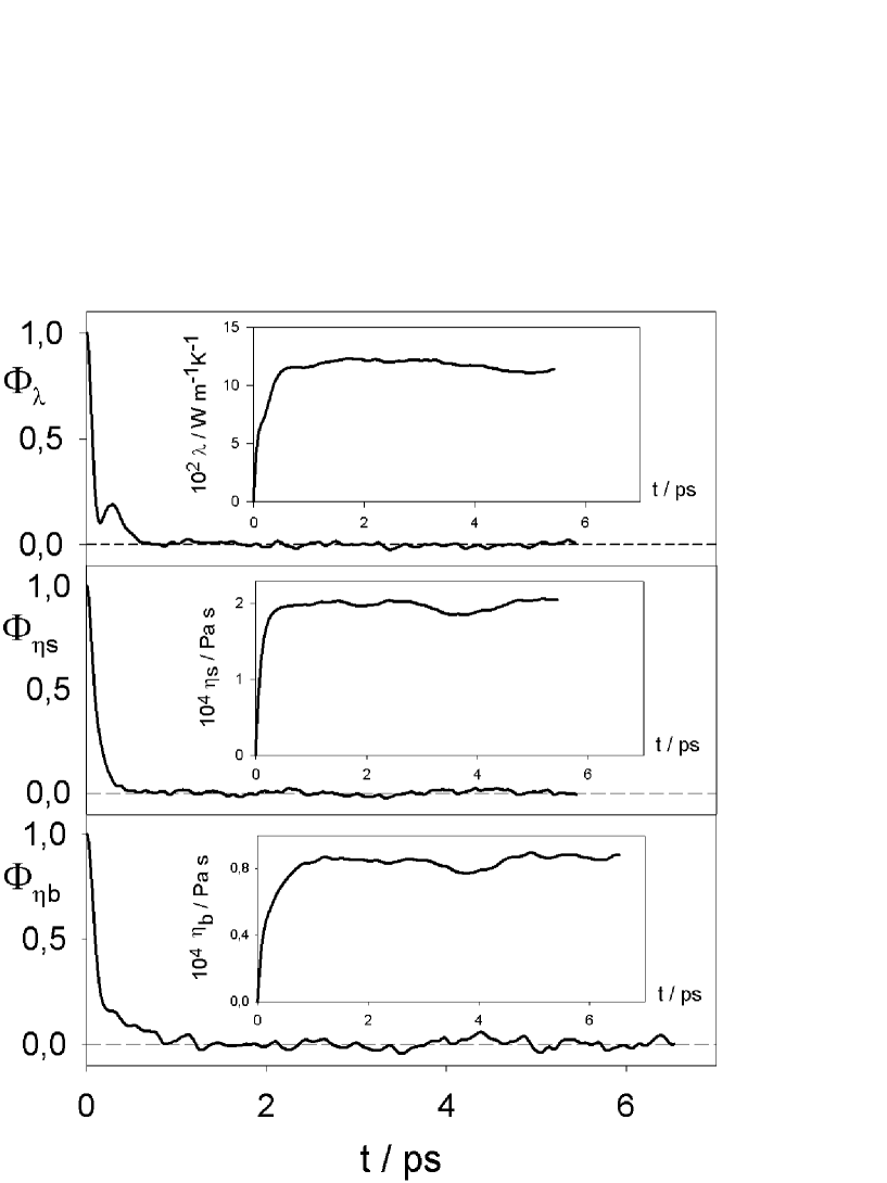
Figure 1:

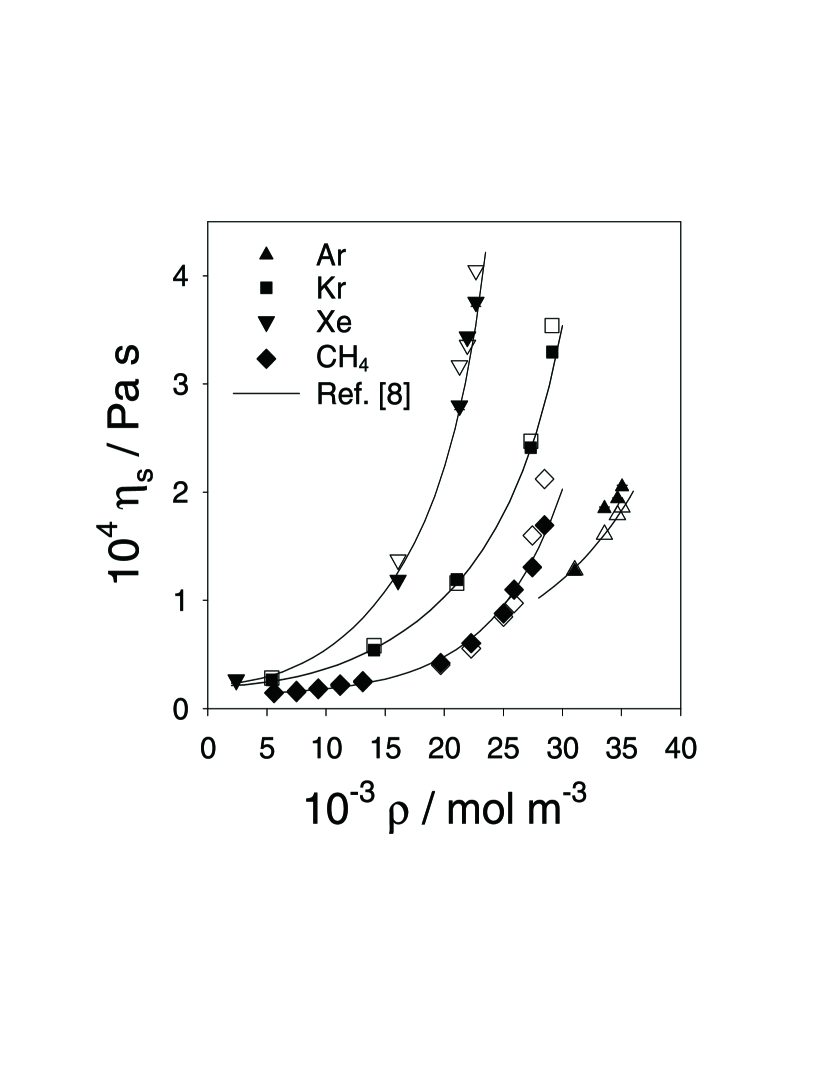
Figure 2:

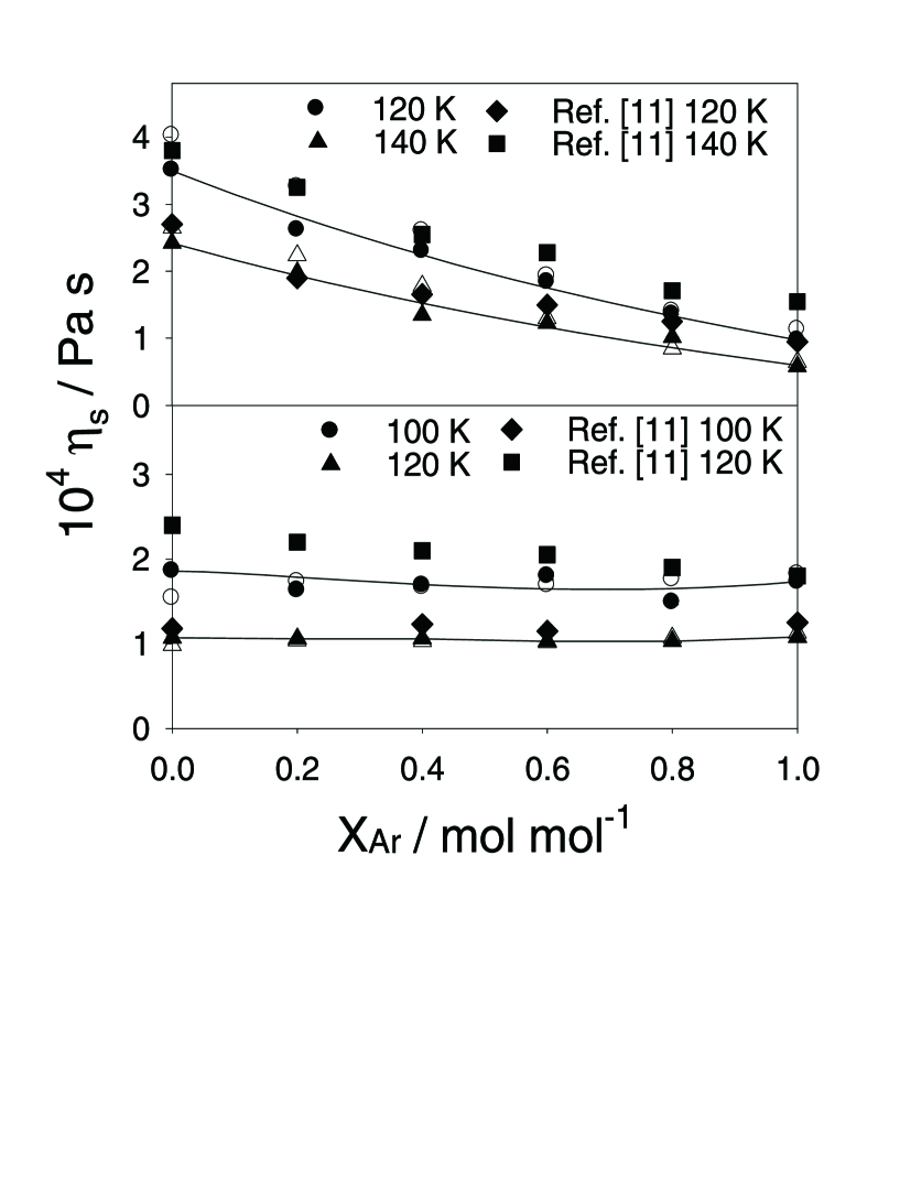
Figure 3:

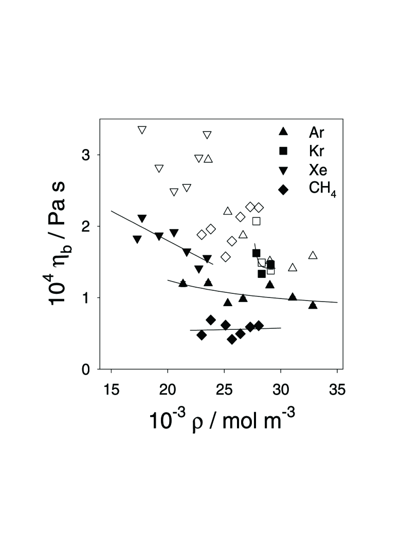
Figure 4:

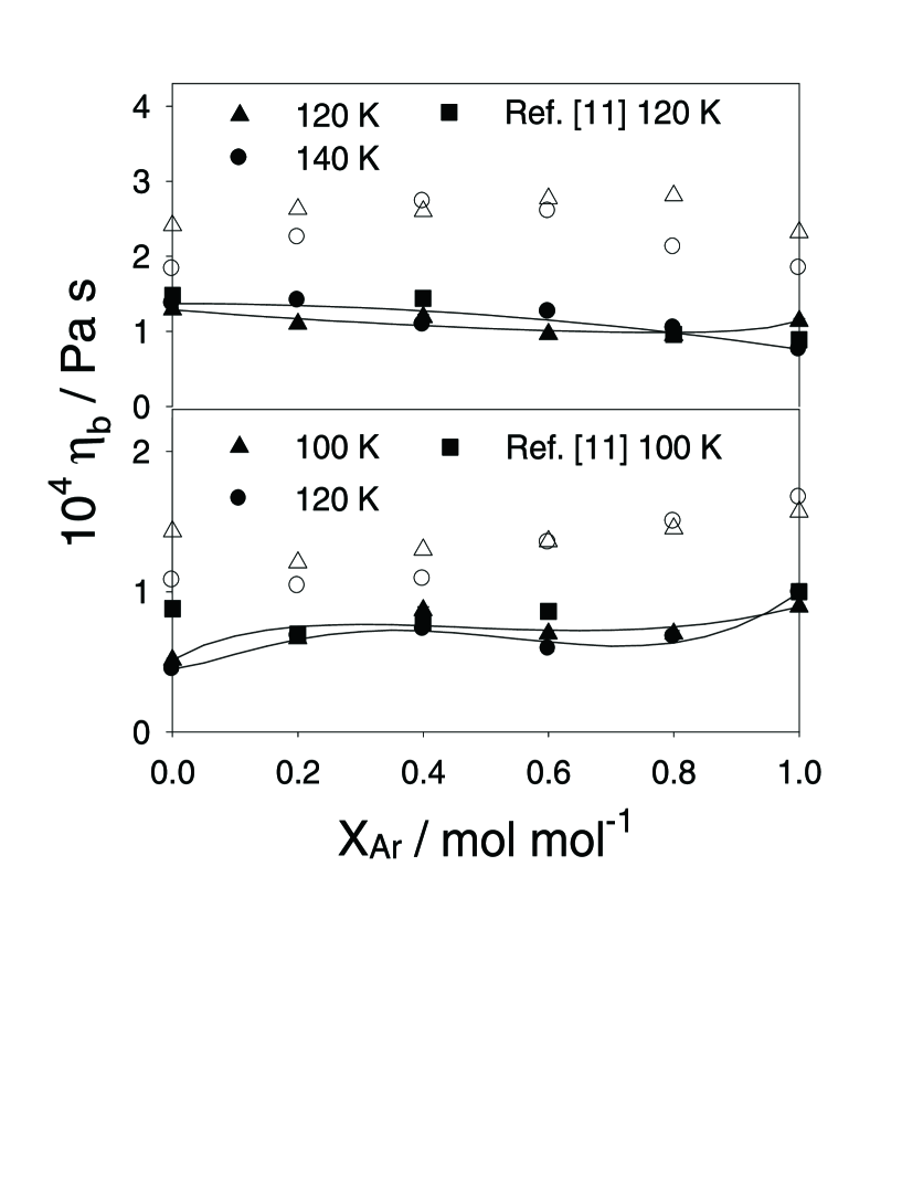
Figure 5:

Figure 6:

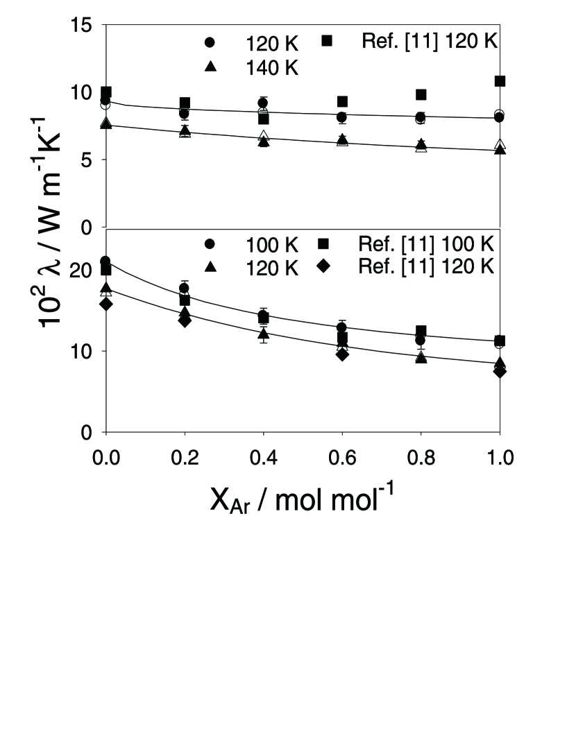
Figure 7:

References

- [1] D.J. Evans, G.P. Morris, Statistical Mechanics of Nonequilibrium Liquids, Academic Press, London 1990.
- [2] M.S. Green, J. Chem. Phys. 22(1954)398-413.
- [3] R. Kubo, J. Phys. Soc. Jpn. 12(1957)570-586.
- [4] B.L. Holian, D.J. Evans, J. Chem. Phys. 78(1983)5147-5150.
- [5] J.J. Erpenbeck, Phys. Rev. A. 35(1987)218-232.
- [6] S.T. Cui, P.T. Cummings, and H.D. Cochran, Mol. Phys. 93(1998)117-121.
- [7] M.F. Pas, and B. Zwolinski, Mol. Phys. 73(1991)483-494.
- [8] R.L. Rowley, M.M. Paiter, Int. J. Thermophys. 18(1997)1109-1121.
- [9] R.L. Rowley, personal comunication. There exist two erros in the cited reference of Rowley et al., it should read: =1067.97, =-2.2065, also the subscript in equation (10) should read instead .
- [10] D.M. Heyes, S.R. Preston, Phys. Chem. Liq. 23(1991)123-149.
- [11] D.M. Heyes, J. Chem. Phys. 96(1992)2217-2227.
- [12] M. Schoen, C. Hoheisel, Mol. Phys. 56(1985)653-672.
- [13] P. Borgelt, C. Hoheisel, and G. Stell, Phys. Rev. A 42(1990)789-794.
- [14] D.M. Heyes, J. Chem. Soc. Faraday Trans. II 80(1984)1363-1394.
- [15] W.G. Hoover, D.J. Evans, R.B. Hickman, W.T. Ashurst, and B. Moran, Phys. Rev. A 22(1980)1690-1697.
- [16] R. Vogelsang, C. Hoheisel, and G. Ciccoti J. Chem. Phys. 35(1987)3487-3491.
- [17] R. Vogelsang, C. Hoheisel, Phys. Rev. A 35(1987)3487-3491.
- [18] K. Meier, A. Laesecke, and S. Kabelac, Int. J. Thermophys. 18(1997)161-173.
- [19] K. Meier, PhD Thesis, Computer Simulation and Interpretation of the Transport Coefficients of the Lennard-Jones Model Fluid, Shaker Publishers, Aachen, 2002.
- [20] J.P.J. Michels, N.J. Trappeniers, Physica A 90(1978)179-195.
- [21] L.A.F. Coelho, J.V. de Oliveira, F.W. Tavares, and M.A. Matthews, Fluid Phase Equilibria 194(2002)1131-1140.
- [22] J.M. Stoker, and R.L. Rowley, J. Chem. Phys. 91(1989)3670-3676.
- [23] J. Vrabec, J. Stoll, and H. Hasse, J. Phys. Chem. B. 48(2001)12126-12133.
- [24] G.A. Fernandez, J. Vrabec, and H. Hasse, Int. J. Thermophys. 25(2004)175-186.
- [25] R. Kubo, Rpts. Progr. Phys., 29(1966)255-284.
- [26] R. Zwanzig, Ann. Rev. Phys. Chem. 12(1965)67-102.
- [27] A.F.M. Baron, The dynamic liquid state, Longman, London, 1974.
- [28] K.E. Gubbins, in K. Singer (Ed.), Statistical Mechanics vol. 1, The Chemical Society, Burlington House, London, 1972, pp 194-253.
- [29] W.A. Steele, in H.J.M. Hanley (Ed.), Transport Phenomena in Fluids, Marcel Dekker, New York and London, 1969, pp 209-312.
- [30] J.O. Hirschfelder, C.F. Curtiss, and R.B. Bird, Molecular Theory of Gases and Liquids, John Wiley & Sons Inc., Ney York, 1954.
- [31] S.M. Karim, Rev. Mod. Phys. 24(1952)108-116.
- [32] S.R. de Groot, P. Mazur, Non-Equilibrium Thermodynamics, Dover, New York, 1984.
- [33] I.R. McDonald, K. Singer, Mol. Phys. 23(1972)29-40.
- [34] J. Vrabec, J. Stoll, and H. Hasse, Molecular models of unlike interaction in mixtures, Int. J. Thermophys, to be submited (2004).
- [35] J. Stoll, J. Vrabec, and H. Hasse. AIChE. J. 49(2003)2187-2198.
- [36] M.P. Allen, D.J. Tildesley, Computer Simulation of Liquids, Clarendon Press, Oxford, 1987.
- [37] J.M. Haile, Molecular Dynamics Simulation, John Wiley & Sons Inc., New York, 1997.
- [38] B.J. Alder, and T.E. Wainwright, Phys. Rev. A 1(1970)18-21.
- [39] D. Fincham, N. Quirke, and D.J. Tildesley, J. Chem. Phys. 84(1986)4535-4546.
- [40] H.C. Andersen, J. Chem. Phys. 72(1980)2384-2393.
- [41] P. Sindzingre, G. Ciccoti, C. Massobrio, and D. Frenkel, Chem. Phys. Lett. 136(1987)35-41.
- [42] N.B. Vargaftik, Y.K. Vinogradov, and V.S. Yargin, Handbook of Physical Properties of Liquids and Gases, Begell house, inc., New York, 1996.
- [43] C. Evers, H.W. Lösch, and W. Wagner, Int. J. Thermophys. 23(2002)1411-1439.
- [44] S.A. Mikhailenko, V.G. Dudar, V.N. Derkach, and V.N. Zozulya, Sov. J. Low. Temp. Phys. 3(1977)331-336.
- [45] S.A. Mikhailenko, V.G. Dudar, and V.N. Derkach, Sov. J. Low. Temp. Phys. 4(1978)205-212.
- [46] J.A. Cowan, R.N. Ball, Can. J. Phys. 50(1972)1881-1886.
- [47] P. Malbrunot, A. Boyer, and E. Charles, Phys. Rev. A 27(1983)1523-1534.
- [48] J.A. Cowan, J.W. Leech, Can. J. Phys. 59(1981)1280-1288.
- [49] J.R. Singer, Can. J. Phys. 51(1969)4729-4733.
- [50] R.E. Graves, J. Thermophysics Heat Transf. 51(1969)4729-4733.
- [51] J. Vrabec, J. Stoll, and H. Hasse, J. Phys. Chem. B 105(2001)12126-12133.
- [52] D.J. Evans, S. Murad, Mol. Phys. 68(1989)1219-1223.
- [53] B.Y. Wang, P.T, Cummings, D.J. Evans, Mol. Phys. 75(1992)1345-1356.
- [54] T. Tokumasu, T. Ohara, and K. Kamijo, J. Chem. Phys. 118(2003)3677-3685.
- [55] B.E. Poling, J.M. Prausnitz, and J.P. O’Connell, The Properties of Gases and Liquids, 5th Edition, McGraw-Hill, New York, 2001.