Stretched-Gaussian asymptotics of the truncated Lévy flights for the diffusion in nonhomogeneous media

Abstract

The Lévy, jumping process, defined in terms of the jumping size distribution and the waiting time distribution, is considered. The jumping rate depends on the process value. The fractional diffusion equation, which contains the variable diffusion coefficient, is solved in the diffusion limit. That solution resolves itself to the stretched Gaussian when the order parameter $\mu\to 2$. The truncation of the Lévy flights, in the exponential and power-law form, is introduced and the corresponding random walk process is simulated by the Monte Carlo method. The stretched Gaussian tails are found in both cases. The time which is needed to reach the limiting distribution strongly depends on the jumping rate parameter. When the cutoff function falls slowly, the tail of the distribution appears to be algebraic.

1 Introduction

Transport in physical systems can be described in terms of a jumping process which is completely defined by two probability distributions. They determine spatial and temporal characteristics of the system and are called the jumping size, $\lambda(x)$, and waiting time, $w(t)$, probability distributions, respectively. The stochastic trajectory consists of infinitely fast jumps which are separated by intervals when the Brownian particle is at rest (e.g., due to traps). Usually, the distributions $\lambda$ and $w$ are regarded as mutually independent and processes which they generate are studied in the framework of the decoupled continuous time random walk (CTRW). If the distribution $w(t)$ is Poissonian, the jumps take place at random, uniformly distributed times and the corresponding process is Markovian. The algebraic form of $w(t)$, which possesses long tails, is of particular interest; it leads to long rests and then to a weak, subdiffusive transport [1]. The jumping size distribution $\lambda$ can assume – in order to be stable – either the Gaussian form, or obey the general Lévy distribution which corresponds to processes with long tails, frequently encountered in many areas of physics, sociology, medicine [2] and many others. In the diffusion limit of small wave numbers, the master equation for the decoupled CTRW, and for the case of the Lévy distributed jumping size, resolves itself to the fractional diffusion equation with a constant diffusion coefficient.

However, many physical phenomena require taking into account that the space has some structure and that the diffusion coefficient must actually be variable. It is the case when one considers the transport in porous, inhomogeneous media and in plasmas, as well as for the Lévy flights in systems with an external potential [3]. In the Hamiltonian systems, the speed of transport depends on regular structures in the phase space [4]. Any description of the diffusion on fractals must involve the variable diffusion coefficient, and that one in the power-law form [5, 6]. Similarly, the diffusion on multifractal structures can be regarded as a superposition of the solutions which correspond to the individual fractals [7]. The power-law form of the diffusion coefficient has been also used to describe e.g. the transport of fast electrons in a hot plasma [8] and the turbulent two-particle diffusion [9]. The presence of long jumps indicates a high complexity and the existence of long-range correlations. One can expect that especially in such systems the waiting time depends on the position. The jumping process, stationary and Markovian, which takes into account that dependence, has been proposed in Ref.[10]: the distribution $w(t)$ is Poissonian with a $x$-dependent jumping rate $\nu(x)$. In this paper, we consider that process for the Lévy distributed $\lambda(x)$ and solve the corresponding fractional equation. The solution consistently takes into account that the symmetric Lévy distribution, defined by the characteristic function $\exp(-|k|^{\mu})$, $0<\mu\leq 2$, exhibits two qualitatively different kinds of behaviour in its asymptotic limit: it is either algebraic, $\sim|x|^{-\mu-1}$, for $0<\mu<2$ or Gaussian for $\mu=2$.

The Lévy process is characterized by very long jumps since the tails of the Lévy distribution fall slowly and the second moment is divergent. In a concrete, realistic problem, however, the available space is finite and the asymptotics differs from the Lévy tail. One can take that into account by introducing a cutoff to the stochastic equations by multiplying the jumping size distribution – in the Lévy form – by a function which falls not slower than $1/|x|^{3}$, usually by the exponential or the algebraic function. Since the resulting probability distribution has the finite variance, in the diffusion approximation the process is equivalent to the Gaussian limit $\mu\to 2$.

Restrictions on the jump size are necessary also for problems connected with the random transport of massive particles. Since the velocity of propagation is then finite, the jump, which takes place within a given time interval, must have a finite length. If the jump size is governed by the particle velocity, a coupling between spatial and temporal characteristics of the system emerges in the framework of CTRW. That coupled form of the CTRW is known as the Lévy walk [11, 12, 13]. It has many applications, e.g. for the turbulence [14] and the chaotic diffusion in Josephson junctions [11].

The aim of this paper is to study the limit in which the algebraic tail of the Lévy process becomes the exponential function. Utilizing the result for $\mu\to 2$ can improve the solution of the fractional equation itself and it is suited to describe the truncated Lévy flights in the diffusion approximation. The paper is organized as follows. In Sec.II we solve the fractional equation and derive the stretched Gaussian asymptotics in the limit $\mu\to 2$. Sec.III is devoted to the truncated Lévy flights: we present the probability distributions, obtained from simulations of random walk trajectories, for both exponential and power-law form of the cutoff. The results are summarized in Sec.IV.

2 The stretched-Gaussian limit of the Lévy process

We consider the random walk process defined by the waiting time probability distribution $w(t)$ and the jump-size distribution $\lambda(x)$. They are of the form

$$w(t)=\nu(x){\mbox{e}}^{-\nu(x)t},$$ (1)

where $\nu(x)=|x|^{-\theta}$ ($\theta>-1$) and

$$\lambda(x)=\sqrt{2/\pi}\int_{0}^{\infty}\exp(-K^{\mu}k^{\mu})\cos(kx)dk,$$ (2)

respectively. The latter expression corresponds to the symmetric Lévy distribution. The master equation for the above process is of the form [10]

$$\frac{\partial}{\partial t}p(x,t)=-\nu(x)p(x,t)+\int\nu(x^{\prime})\lambda(|x-x^{\prime}|)p(x^{\prime},t)dx^{\prime}.$$ (3)

In the diffusion limit of small wave numbers, the Eq.(3) can be reduced to the fractional equation. Indeed, the Fourier transform of jump-size distribution, ${\widetilde{\lambda}}(k)=\exp(-K^{\mu}|k|^{\mu})$, can be expanded ${\widetilde{\lambda}}(k)=1-K^{\mu}|k|^{\mu}+\dots$ and the master equation in the Fourier space becomes the following equation [15]

$$\frac{\partial{\widetilde{p}}(k,t)}{\partial t}=-K^{\mu}|k|^{\mu}{\widetilde{F}}[\nu(x)p(x,t)].$$ (4)

The above approximation means that the summation over jumps is substituted by the integral and it agrees with the exact result if the jumps are small, compared to the entire trajectory. One can demonstrate by estimating the neglected terms in the Euler-Mclaurin summation formula that the approximation fails near the origin and for $\mu\leq 1$ [16]. In the other cases, the solution of the fractional equation converges with time to the exact result. Therefore, in the following, we assume $\mu>1$.

The inversion of the Fourier transforms in Eq.(4) yields the fractional equation

$$\frac{\partial p(x,t)}{\partial t}=K^{\mu}\frac{\partial^{\mu}[\nu(x)p(x,t)]}{\partial|x|^{\mu}},$$ (5)

where $\partial^{\mu}/\partial|x|^{\mu}$ is the Riesz-Weyl derivative, defined for $1<\mu<2$ in the following way [17]

$$\frac{\partial^{\mu}}{\partial|x|^{\mu}}f(x,t)=\frac{-1}{2\cos(\pi\mu/2)\Gamma(2-\mu)}\frac{\partial^{2}}{\partial x^{2}}\int_{-\infty}^{\infty}\frac{f(x^{\prime},t)}{|x-x^{\prime}|^{\mu-1}}dx^{\prime}.$$ (6)

Eq.(5) for the constant diffusion coefficient – often generalized to take into account non-Markovian features of the trapping mechanism in the framework of CTRW by substituting the simple time derivative by the fractional Riemann-Liouville derivative [1] – is frequently considered and solved by means of a variety of methods. The solution resolves itself to the Lévy stable distribution with the asymptotic power-law $x$-dependence and divergent second moment. The method of solution which is especially interesting for our considerations involves the Fox functions. The well-known result of Schneider [18] states that any Lévy distribution, both symmetric and asymmetric, can be expressed as $H_{2,2}^{1,1}$. In order to solve the Eq.(5) for the case of the variable jumping rate, $\nu(x)=|x|^{-\theta}$, we conjecture that the solution also belongs to the class of functions $H_{2,2}^{1,1}$ and it has the scaling property. Then the ansatz is the following

$$p(x,t)=Na(t)H_{2,2}^{1,1}\left[a(t)|x|\left|\begin{array}[]{c}(a_{1},A_{1}),(a_{2},A_{2})\\ \\ (b_{1},B_{1}),(b_{2},B_{2})\end{array}\right.\right],$$ (10)

where $N$ is the normalization constant. The Fox function is defined in the following way [19, 20]

$$H_{pq}^{mn}\left[z\left|\begin{array}[]{c}(a_{p},A_{p})\\ \\ (b_{q},B_{q})\end{array}\right.\right]=\frac{1}{2\pi i}\int_{L}\chi(s)z^{s}ds,$$ (14)

where

$$\chi(s)=\frac{\prod_{1}^{m}\Gamma(b_{j}-B_{j}s)\prod_{1}^{n}\Gamma(1-a_{j}+A_{j}s)}{\prod_{m+1}^{q}\Gamma(1-b_{j}+B_{j}s)\prod_{n+1}^{p}\Gamma(a_{j}-A_{j}s)}.$$ (15)

The contour $L$ separates the poles belonging to the two groups of the gamma function in the Eq.(15). Evaluation of the residues leads to the well-known series expansion of the Fox function:

$$\hskip-28.45274ptH_{pq}^{mn}\left[z\left|\begin{array}[]{c}(a_{p},A_{p})\\ \\ (b_{q},B_{q})\end{array}\right.\right]=\sum_{h=1}^{m}\sum_{\nu=0}^{\infty}\frac{\prod_{j=1,j\neq h}^{m}\Gamma(b_{j}-B_{j}\frac{b_{h}+\nu}{B_{h}})\prod_{j=1}^{n}\Gamma(1-a_{j}+A_{j}\frac{b_{h}+\nu}{B_{h}})}{\prod_{j=m+1}^{q}\Gamma(1-b_{j}+B_{j}\frac{b_{h}+\nu}{B_{h}})\prod_{j=n+1}^{p}\Gamma(a_{j}-A_{j}\frac{b_{h}+\nu}{B_{h}})}\frac{(-1)^{\nu}z^{(b_{h}+\nu)/B_{h}}}{\nu!B_{h}},$$ (19)

We will try to solve the fractional equation (5) by inserting the function (10). This procedure, if successful, would allow us to find conditions for the coefficients and the function $a(t)$. The idea to assume the solution in the form (10) is motivated by the following property of the Fox function

$$z^{\sigma}H_{pq}^{mn}\left[z\left|\begin{array}[]{c}(a_{p},A_{p})\\ \\ (b_{q},B_{q})\end{array}\right.\right]=H_{pq}^{mn}\left[z\left|\begin{array}[]{c}(a_{p}+\sigma A_{p},A_{p})\\ \\ (b_{q}+\sigma B_{q},B_{q})\end{array}\right.\right]$$ (26)

which eliminates the algebraic factor by means of a simple shift of the coefficients. One can demonstrate that Eq.(5) cannot be satisfied, in general, by the function (10) for any choice of the parameters. However, as long as we are interested only in the diffusion limit of small wave numbers $|k|$ (large $|x|$), the higher terms in the characteristic function expansion can be neglected. Therefore we require that the Eq.(5) should be satisfied by a function which agrees with the exact solution only up the terms of the order $|k|^{\mu}$ in the Fourier space. Note that this condition does not introduce any additional idealization since the Eq.(5) itself has been constructed on the same assumption: the higher terms in the $|k|$ expansion of $\lambda(x)$ have been also neglected.

First, we need the Fourier transform of the Fox function. Since the process is symmetric, we can utilize the formula for the cosine transform which yields also a Fox function but of the enhanced order:

$$\hskip-28.45274pt\int_{0}^{\infty}H_{pq}^{mn}\left[x\left|\begin{array}[]{c}(a_{p},A_{p})\\ \\ (b_{q},B_{q})\end{array}\right.\right]\cos(kx)dx=\frac{\pi}{k}H_{q+1,p+2}^{n+1,m}\left[k\left|\begin{array}[]{l}(1-b_{q},B_{q}),(1,1/2)\\ \\ (1,1),(1-a_{p},A_{p}),(1,1/2)\end{array}\right.\right].$$ (33)

The function ${\widetilde{p}}(k,t)$ is then of the order $H_{3,4}^{2,1}$. The Fourier transform of the function $p_{\theta}=x^{-\theta}p(x,t)$ can be obtained in the same way. Next, we insert the appropriate functions into the Eq.(4) and expand both sides of the equation by using the formula (19). Let us denote the expansion coefficients of the functions ${\widetilde{p}}(k,t)$ and ${\widetilde{p}_{\theta}}(k,t)$ by $h_{\sigma,\nu}$ and $h_{\sigma,\nu}^{(\theta)}$, respectively; $\sigma$ assumes the values 1 and 2. Applying the Eq.(19) yields

$${\widetilde{p}}(k,t)=h_{1,0}+h_{1,1}|k|+h_{2,0}|k|^{(1-a_{1})/A_{1}-1}+h_{2,1}|k|^{(2-a_{1})/A_{1}-1}+h_{1,2}k^{2}+\dots$$ (34)

and

$${\widetilde{p}_{\theta}}(k,t)=h_{1,0}^{(\theta)}+h_{1,1}^{(\theta)}|k|+h_{2,0}^{(\theta)}|k|^{(1-a_{1}+\theta A_{1})/A_{1}-1}+\dots.$$ (35)

After inserting the above expressions to the Eq.(4), we find some simple relations among the coefficients of the Fox function by comparison of the exponents. To get the term $|k|^{\mu}$ on lhs, which corresponds to the term $k^{0}$ on rhs, we need the condition $(2-a_{1})/A_{1}-1=\mu$. Moreover, we attach the third term on rhs to the first one by putting $(1-a_{1}+\theta A_{1})/A_{1}-1=0$; it is not possible to balance the third term by another one on the lhs. The above conditions determine two coefficients of the Fox function: $a_{1}=1-(1-\theta)/(\mu+\theta)$ and $A_{1}=1/(\mu+\theta)$. The coefficients $h_{1,1}$ and $h_{1,1}^{(\theta)}$ vanish identically since the gamma function in the denominators has its argument equal 0. The only remaining term can be eliminated by assuming the condition $1-b_{2}-B_{2}(1-\theta)=0$; then $h_{2,0}=0$ since that term contains the function $\Gamma(1-b_{2}-B_{2}(1-\theta))$ in the denominator. Therefore, such choice of the coefficients reduces the function (34) to the two terms and it makes it identical with the probability distribution for the Lévy process in the diffusion limit. Finally, the Eq.(4) becomes a simple differential equation which determines the function $a(t)$:

$$\dot{\xi}=K^{\mu}\frac{h_{0}^{(\theta)}}{h_{2,1}}\xi^{-\theta/\mu},$$ (36)

where $h_{0}^{(\theta)}=h_{1,0}^{(\theta)}+h_{2,0}^{(\theta)}$ and $\xi(t)=a^{-\mu}$. The solution

$$a(t)=\left[K^{\mu}\frac{h_{0}^{(\theta)}}{h_{2,1}}\left(1+\frac{\theta}{\mu}\right)t\right]^{-1/(\mu+\theta)}$$ (37)

corresponds to the initial condition $p(x,0)=\delta(x)$. The coefficient $h_{2,1}$ can be determined directly from Eq.(19), whereas $h_{0}^{(\theta)}=(2\pi)^{-1}a^{-\theta}{\widetilde{p}}(0,t)=\pi^{-1}a^{-\theta}\int_{0}^{\infty}p(x,t)dx$ can be expressed in terms of the Mellin transform from the Fox function, $\chi(s)$, and then easily evaluated.

In the limit $\mu\to 2$, the asymptotic behaviour of the fractional equation changes qualitatively. It is no longer algebraic; the tails of the distribution, and consequently the tails of the Fox function, have to assume the exponential form for $\mu=2$. It is possible only if the algebraic contribution from the residues vanishes. If $n=0$, all poles are outside the contour $L$ and $H_{p,q}^{m,0}$ is given by the integral over a vertical straight line:

$$H_{p,q}^{m,0}=\frac{1}{2\pi i}\int_{w-i\infty}^{w+i\infty}\chi(s)z^{s}ds,$$ (38)

where $w<Re(b_{i}/B_{i})$. The above integral is usually neglected if $n>0$ because it is small compared to the contribution from the residues.

The Fox function in the required form can be obtained from (10) by applying the reduction formula if the coefficients in the main diagonal are equal. This demand imposes an additional condition on $b_{2}$ and $B_{2}$ which allows us to determine these coefficients: $b_{2}=1-(1-\theta)/(2+\theta)$ and $B_{2}=1/(2+\theta)$. Note that the above choice of $(b_{2},B_{2})$ yields $h_{1,2}=0$ in Eq.(34) and then the solution of Eq.(5) is exact up to the order $k^{2}$ for any $\mu$. The most general solution of the fractional equation in the form of the function $H^{1,1}_{2,2}$, which involves the required conditions, is the following

$$p(x,t)=Na(t)H_{2,2}^{1,1}\left[a(t)|x|\left|\begin{array}[]{c}(1-\frac{1-\theta}{\mu+\theta},\frac{1}{\mu+\theta}),(a_{2},A_{2})\\ \\ (b_{1},B_{1}),(1-\frac{1-\theta}{2+\theta},\frac{1}{2+\theta})\end{array}\right.\right].$$ (42)

The coefficients in the main diagonal have a simple interpretation. Applying Eq.(19) to (42) reveals that $p(x,t)$ behaves as $|x|^{b_{1}/B_{1}}$ for $|x|\to 0$ and then the parameters $b_{1}$ and $B_{1}$ are responsible for the shape of the probability distribution near the origin. On the other hand, the parameters $a_{1}$ and $A_{1}$ determine the asymptotic shape of the distribution. It can be demonstrated by applying the following property of the Fox function

$$H_{pq}^{mn}\left[z\left|\begin{array}[]{c}(a_{p},A_{p})\\ \\ (b_{q},B_{q})\end{array}\right.\right]=H_{pq}^{mn}\left[\frac{1}{z}\left|\begin{array}[]{c}(1-b_{q},B_{q})\\ \\ (1-a_{p},A_{p})\end{array}\right.\right]$$ (49)

and by expansion according to Eq.(19): the leading term is of the form $p(x,t)\sim|x|^{(2-a_{1})/A_{1}}=|x|^{-1-\mu}~{}~{}~{}~{}(|x|\to\infty)$. Now it becomes clear why our method of solving the Eq.(5) did not determine the parameters $(b_{1},B_{1})$. Since we neglected higher terms in the $k$-expansion, the region of small $|x|$ remained beyond the scope of the approximation. However, we can supplement that solution by referring directly to the master equation (3) which reveals a simple behaviour near the origin. That equation is satisfied by the stationary solution $1/\nu(x)=|x|^{\theta}$, for any normalizable $\lambda(x)$. Obviously, such $p(x,t)$ cannot be interpreted as the probability density distribution since the normalization integral diverges in infinity but it properly reproduces that distribution for small $|x|$. Therefore we obtain the additional condition $b_{1}=\theta B_{1}$ which improves the agreement of our solution with the solution of the master equation. The probability distribution for the case $\theta=0$ can be easily found by the direct solution of the fractional equation which is exact and yields the following values of the parameters: $b_{1}=0$, $B_{1}=1$, $a_{2}=1/2$, and $A_{2}=1/2$.

In the case $\mu=2$, the main diagonal in Eq.(42) can be eliminated and the solution of the fractional equation (5) in the limit $\mu\to 2$ takes the form

$$p(x,t)=Na(t)H_{1,1}^{1,0}\left[a(t)|x|\left|\begin{array}[]{c}(a_{2},A_{2})\\ \\ (b_{1},B_{1})\end{array}\right.\right].$$ (53)

The function $a(t)$ is given by Eq.(37) in the following form

$$a(t)=\left[K^{2}(2+\theta)\frac{h_{0}}{h_{2}}t\right]^{-1/(2+\theta)},$$ (54)

where $h_{0}=\Gamma(b_{1}+B_{1}(1-\theta))/\Gamma(a_{2}+A_{2}(1-\theta))$ and $h_{2}=\Gamma(b_{1}+3B_{1})/\Gamma(a_{2}+3A_{2})$ are the coefficients of the $k$-expansion of the functions $|x|^{-\theta}p(x,t)$ and $p(x,t)$, respectively. The asymptotic expression for $p(x,t)$ can be obtained from the estimation of the integral (38) by the method of steepest descents [21]. The result reads

$$H_{1,1}^{1,0}(z)\approx{\mbox{e}}^{i\pi(\alpha^{\prime}-1/2)}E(z{\mbox{e}}^{i\pi\alpha}),$$ (55)

where

$$E(z)=\frac{1}{2\pi i\alpha}\sum_{j=0}^{\infty}C_{j}(\beta\alpha^{\alpha}z)^{(1-\alpha^{\prime}-j)/\alpha}\exp(\beta\alpha^{\alpha}z)^{1/\alpha}$$ (56)

and $\alpha=B_{1}-A_{2}$, $\alpha^{\prime}=a_{2}-b_{1}+1/2$, $\beta=A_{2}^{A_{2}}/B_{1}^{B_{1}}$, $z=a|x|$. The final result appears to be a stretched Gaussian, modified by an algebraic factor and a series which converges to a constant for $z\to\infty$:

$$H_{1,1}^{1,0}(z)\approx\frac{1}{2\pi\alpha}z^{(1-\alpha^{\prime})/\alpha}\exp(-\beta^{1/\alpha}\alpha z^{1/\alpha})\beta^{(1-\alpha^{\prime})/\alpha}\alpha^{1-\alpha^{\prime}}\sum_{j=0}^{\infty}(-1)^{j}C_{j}\beta^{-j/\alpha}\alpha^{-j}z^{-j/\alpha}.$$ (57)

The above expression has been obtained by Wyss [22] as the expansion of $H^{3,0}_{2,3}(z)$ which satisfies a generalized diffusion equation. It is the integral equation in respect to the time variable (non-Markovian) which resolves itself to the fractional diffusion equation; that equation is commonly used to handle the subdiffusive processes in the framework of the CTRW [12, 23, 1]. The function which contains the stretched Gaussian, modified by the power-law factor, is used as the asymptotic form of the propagator for diffusion on fractals, e.g. on the Sierpiński gasket [24].

The coefficients $C_{j}$ are defined by means of the following expression

$$\frac{\Gamma(1-a_{2}+A_{2}s)}{\Gamma(1-b_{1}+B_{1}s)}(\beta\alpha^{\alpha})^{-s}\equiv G=\sum_{j=0}^{\infty}\frac{C_{j}}{\Gamma(\alpha s+\alpha^{\prime}+j)}.$$ (58)

They can be explicitly evaluated by a subtraction of the consecutive terms and by taking the limit $s\to\infty$. More precisely, $C_{j}$ are given by the following recurrence formula

$$\hskip-28.45274ptC_{j} = \lim_{s\to\infty}\left[G\Gamma(\alpha s+\alpha^{\prime})-C_{0}-\frac{C_{1}}{\alpha s+\alpha^{\prime}}-\dots-\frac{C_{j}}{(\alpha s+\alpha^{\prime})\dots(\alpha s+\alpha^{\prime}+j-1)}\right]\times$$ (59)

$$\times (\alpha s+\alpha^{\prime})(\alpha s+\alpha^{\prime}+1)\dots(\alpha s+\alpha^{\prime}+j-1)$$

where

$$C_{0}=\sqrt{2\pi}\alpha^{\alpha^{\prime}-1/2}A_{2}^{1/2-a_{2}}B_{1}^{b_{1}-1/2}$$ (60)

has been obtained from the expansion of the gamma functions by means of the Stirling formula. The exponent of the stretched Gaussian, $1/\alpha$, is connected with higher moments of the distribution $p(x,t)$ and it cannot be determined in the framework of the diffusion approximation.

All moments of the distribution $p(x,t)$ are convergent. In particular, the variance, which determines the diffusion properties of the system, is given by the expansion coefficient $h_{2}$ in a simple way:

$$\langle x^{2}\rangle=-\frac{\partial^{2}}{\partial k^{2}}{\widetilde{p}}(0,t)=h_{2}a^{-2}\sim t^{\frac{2}{2+\theta}}.$$ (61)

For $\theta=0$ the diffusion coefficient $D=\lim_{t\to\infty}\langle x^{2}\rangle(t)/2t$ assumes a finite value and the diffusion is normal. The case $\theta\neq 0$ means the anomalous diffusion: either the enhanced one for $\theta<0$, or the subdiffusion for $\theta>0$; the diffusion coefficients are then $\infty$ or 0, respectively. The kind of diffusion depends only on $\theta$ and it is not sensitive on free parameters. The anomalous diffusion is frequently encountered in physical phenomena, in particular in complex and disordered systems [25], as well as in dynamical systems [4].

On the other hand, the fractional equation (5) for $\mu=2$ assumes a form of the simple diffusion equation

$$\frac{\partial p(x,t)}{\partial t}=K^{2}\frac{\partial^{2}[|x|^{-\theta}p(x,t)]}{\partial x^{2}}$$ (62)

which can be solved exactly just by assuming the scaling form of the solution $p(x,t)=a(t)f(a(t)x)$. The functions $a(t)$ and $f(ax)$ are derived by inserting to the Eq.(62) and by separation of the variables [26]. That procedure finally yields

$$p(x,t)=N(K^{2}t)^{-\frac{1+\theta}{2+\theta}}|x|^{\theta}\exp\left(-\frac{|x|^{2+\theta}}{K^{2}(2+\theta)^{2}t}\right).$$ (63)

Eq.(62) follows from the master equation (3) with the Gaussian $\lambda(x)$, when one neglects all terms higher than the second one in the Kramers-Moyal expansion. That procedure is justified if jumps are small and $\nu(x)$ is a smooth function [27]. We can expect that the solution of the master equation converges with time to Eq.(63) and this convergence is fast for small $|\theta|$. Convergence of the tails must be slow, because the contribution from large jumps is substantial for large $|x|$. Indeed, we will demonstrate in the following that for large $|\theta|$, in particular for $\theta$ close to $-1$, a very long time is required.

The result (63) is useful for further improvement of the solution (42). The comparison of Eqs. (57) and (63) yields the conditions for the Fox function coefficients which ensure the proper limit $\mu\to 2$: $\lim_{\mu\to 2}(B_{1}-A_{2})=1/(2+\theta)$ and $\lim_{\mu\to 2}(1-\alpha^{\prime})/\alpha=\theta$. By inserting the coefficients which follow from those limiting values to the Eq.(42) and by assuming, in addition, that $B_{1}=1$, we obtain a particular solution of the fractional equation (5) in the form

$$p(x,t)=Na(t)H_{2,2}^{1,1}\left[a(t)|x|\left|\begin{array}[]{c}(1-\frac{1-\theta}{\mu+\theta},\frac{1}{\mu+\theta}),(\frac{1}{2}+\frac{\theta(1+\theta)}{2+\theta},1-\frac{1}{2+\theta})\\ \\ (\theta,1),(1-\frac{1-\theta}{2+\theta},\frac{1}{2+\theta})\end{array}\right.\right].$$ (67)

Therefore, the above solution of the fractional equation takes into account the Kramers-Moyal result (63) in the limit $\mu\to 2$ and its behaviour in the origin agrees with the master equation. The limit $\theta\to 0$ corresponds to the Lévy process.

3 Truncated Lévy flights

The Lévy flights are characterized by the power-law tail with the exponent smaller than 3 which implies the infinite variance. However, in physical systems, which are limited in space, the variance must always be finite. The finiteness of the available space must be taken into account in any attempt to simulate the random walk in lattices, for example, in a model of turbulence which describes a transport in a Boltzmann lattice gas [28]. One can constrain the jumping size either by taking into account that the Brownian particle actually possesses a finite velocity, i.e. to substitute the Lévy flights by the Lévy walks, or by introducing some cutoff in the jumping size probability distribution. As a result, the variance becomes finite and, in the case of the mutually independent jumps, the random walk probability distribution converges to the Gaussian, according to the central limit theorem. The truncation of the Lévy flights can be accomplished either by a simple removing of the tail [29] or by multiplying the tail by some fast falling function. An obvious choice in this context is the exponential $\exp(-\gamma|x|)$ and the algebraic function $|x|^{-\beta}$, where $\beta\geq 2-\mu$. The former case was considered by Koponen in Ref.[30], where an analytic expression for the characteristic function was derived. The Lévy flights with exponential truncation serve as a model for phenomena in many fields, e.g. in turbulence [31], solar systems, economy. The distribution function of velocity and magnetic-field vector differences within solar wind can be reasonably fitted in this way [32]. In the framework of the economic research, the Lévy process is a natural model of the financial assets flow and the fractional equations are applied to characterize the dynamics of stock prices, where rare, non-Gaussian events are frequently encountered, in particular if the market exhibits high volatility. One can improve in this way the Black-Scholes model, commonly used to price the options, which is restricted to the Gaussian distributions. In order to incorporate the finiteness of the financial system to the fractional equations formalism by means of the exponential truncation of the Lévy tails, models known as CGMY and KoBoL have been devised [33]. The non-Markovian fractional equation, which results from the CTRW model with the Lévy distributed and exponentially truncated jump size, has been considered in Ref.[34]. The solutions do not exhibit a typical scaling at small time but they converge, asymptotically, to the stretched Gaussian which is predicted by the subdiffusive case of CTRW with the Gaussian step-size distribution.

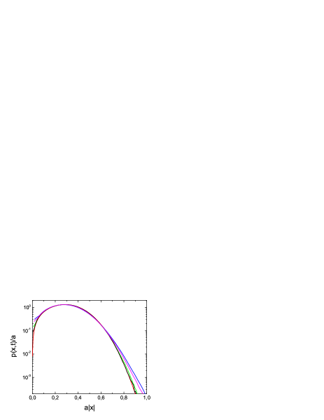
Figure 1: The distributions $p(x,t)$ obtained from trajectory simulations for the power-law cutoff (71) with $\mu^{\prime}=5.5$ for $t=5$, $t=10$, $t=50$ and $t=200$ (from top to bottom). The distribution predicted by Eq.(63) is also presented and it coincides with the curve for $t=200$. Other parameters are the following: $\theta=1$, $\sigma=0.1$ and $a=t^{-1/(2+\theta)}$.

In Ref. [30], the following jumping size distribution, in the form of the Lévy tail multiplied by the exponential factor, has been introduced:

$$\lambda(x)=N{\mbox{e}}^{-\gamma|x|}|x|^{-\mu-1}$$ (68)

and the characteristic function for the process has been evaluated. In the above formula $\gamma\geq 0$ and $N$ is the normalization constant. For the symmetric process, the normalized Fourier transform from $\lambda(x)$ is given by [30, 34]

$${\widetilde{\lambda}(k)}=\frac{4}{\pi}\mu\Gamma(\mu)\tan(\pi\mu/2)[\gamma^{\mu}-(k^{2}+\gamma^{2})^{\mu/2}\cos(\mu\arctan(k/\gamma)]+1.$$ (69)

We keep only the terms of the lowest order in $|k|$. The expansion of the expression (69) produces the following result

$${\widetilde{\lambda}(k)}\approx 1+\frac{2}{\pi}\mu\Gamma(\mu)\gamma^{\mu-2}\tan(\pi\mu/2)(\mu^{2}-\mu)k^{2}\equiv 1-K_{E}^{2}k^{2}.$$ (70)

The diffusion process is then described by Eq.(62) with $K^{2}=K_{E}^{2}$.

Figure 2: The time $T$ needed to reach the distribution (63), as a function of $\theta$, for the case of the algebraic cutoff (71) with the parameters $\mu^{\prime}=5.5$ and $\sigma=0.1$.

On the other hand, one can apply the power-law cutoff to the Lévy tail. In Ref.[35] the fractional equation of the distributed order, with the constant diffusion coefficient, was introduced; it implies the cutoff in the form of the power-law function with the exponent $5-\mu$. Since the equation involves both the fractional and the diffusion component, there is no simple scaling. In this paper, we assume the jumping size distribution in the form of the modified Lévy tail:

$$\lambda(x)=\left\{\begin{array}[]{ll}0&\mbox{for $|x|\leq\sigma$}\\ \mu^{\prime}\sigma^{\mu^{\prime}}|x|^{-\mu^{\prime}-1}&\mbox{for $|x|>\sigma$},\end{array}\right.$$ (71)

where $\mu^{\prime}=\mu+\beta>2$ to ensure the existence of the second moment. The Fourier transform is given by [36]

$${\widetilde{\lambda}(k)}=1-\frac{\mu^{\prime}}{2(\mu^{\prime}-2)}(k\sigma)^{2}-\left[\Gamma(1-\mu^{\prime})\cos(\pi\mu^{\prime}/2)\right](|k|\sigma)^{\mu^{\prime}}+\dots.$$ (72)

In this case we have $K^{2}=\mu^{\prime}\sigma^{2}/2(\mu^{\prime}-2)$, provided we keep only the quadratic term.

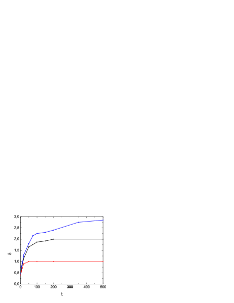
Figure 3: The shape parameter $\delta$ of the distribution tail $\exp(-const|ax|^{\delta})$ as a function of time for the exponential cutoff (68). The curves correspond to the cases: $\theta=1$, $\theta=0$ and $\theta=-0.5$ (from top to the bottom). The other parameters: $\mu=1.5$ and $\gamma=1$.

In the following, we evaluate the probability density distribution $p(x,t)$ for both forms of the Lévy flight cutoff, exponential and algebraic, by means of the random walk trajectory simulations. The waiting time is sampled from Eq.(1) and the jumping size from either (68) or (71). Fig.1 presents the power-law case for $\theta=1$, which corresponds to the subdiffusion. The results are compared with the Kramers-Moyal limiting distribution (63), which is expected to be reached at large time. We observe a rapid convergence for small and medium $|x|$-values, whereas the tails reach the form (63) at about $t=200$. Nevertheless, the shape of the tails is always stretched exponential $\sim\exp(-const|ax|^{\delta})$ and the index $\delta$ rises with time. The speed of convergence to the distribution (63) strongly depends on the parameter $\theta$. In Fig.2 we present the convergence time $T$ as a function of $\theta$. It is relatively short only for small $|\theta|$; for this case the kernel in the master equation (3) changes weakly with $|x|$ and the higher terms in the Kramers-Moyal expansion soon become negligible. $T$ rises rapidly for the negative $\theta$: the estimation presented in the figure suggests that the dependence $T(\theta)$ is exponential, $\sim\exp(-16\theta)$, which yields $T\sim 10^{8}$ when $\theta$ approaches -1. The rapid growth of the time needed to reach convergence of the tails for the negative $\theta$ may also be related to a specific shape of the distribution. The tails become flat for $\theta<0$, and the asymptotics emerges first for very large $|x|$. On the other hand, the probability density to stay in the origin, $p(0,t)$, is then infinite: we have $p(x,t)\sim t^{-(1+\theta)/(2+\theta)}|x|^{\theta}$ $(|x|\ll 1)$, according to Eq.(63). Note that in the case $\theta=0$ we obtain the usual result for diffusion: $p(0,t)\sim 1/\sqrt{t}$.

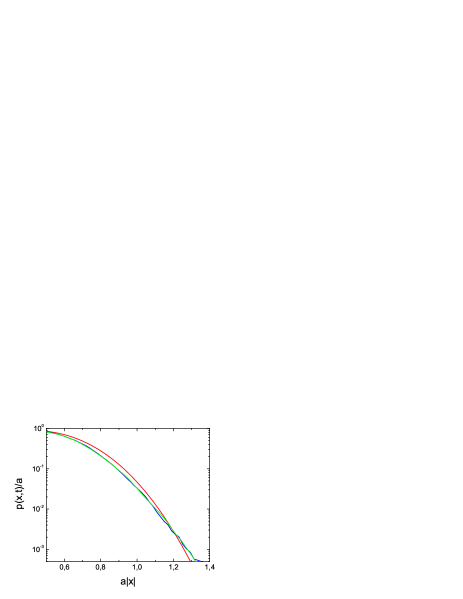
Figure 4: The distributions $p(x,t)$ at $t=100$ and $t=200$ obtained from trajectory simulations for the exponential cutoff with $\mu=1.5$ and $\gamma=2$. These curves coincide and assume the numerically estimated shape $\sim a|x|\exp(-4.7(a|x|)^{2.6}$. The distribution predicted by Eq.(63) is also presented. The parameter $\theta=1$ and $a=t^{-1/(2+\theta)}$.

Application of the exponential cutoff to the Lévy tail produces similar probability density distributions to those presented in Fig.1 and they are also characterized by the stretched Gaussian tails. However, the convergence rate of the index $\delta$ to the value $2+\theta$, predicted by the solution (63), is smaller than for the power-law truncation because the kernel in Eq.(3) is steeper in this case. In Fig.3 we present the dependence $\delta(t)$ for all kinds of the diffusion. Initially, the exponent rises fast but then it begins to stabilize and the curves approach the asymptotic values very slowly, especially for the superdiffusive case of the negative $\theta$. Discrepancies from Eq.(63) are more pronounced for $\gamma=2$. This case is presented in Fig.4: though the rescaled distribution seems to be stabilized already for $t=100$, its shape differs from (63) also for intermediate values of $a|x|$.

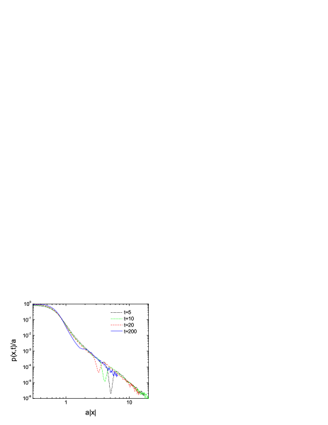
Figure 5: The distributions $p(x,t)$, plotted in the double logarithmic scale, obtained from trajectory simulations for the power-law cutoff with $\mu^{\prime}=2.5$, $\theta=1$ and $\sigma=0.1$.

The exponential asymptotics of the probability density distributions is guarantied by the existence of the finite second moment. However, the time needed to reach that asymptotics can be so large [29] that it cannot be observed in any practical realizations of the process. In fact, the convergence rate to the normal distribution is governed by the third moment, according to the Berry-Esséen theorem [37] which refers to the sum of mutually independent variables, sampled from the same distribution. It states that if the third moment $\rho$ is finite, then the deviation of a given distribution from the normal one is less than $33\rho/(4\sigma^{3}\sqrt{n})$, where $n$ the number of steps and $\sigma$ is the standard deviation. If $\rho=\infty$, the convergence to the Gaussian may be problematic in practice. To demonstrate that the case of divergent third moment is exceptional also for our process, let us consider the power-law cutoff of the Lévy tail, Eq.(71), with the parameter $\mu^{\prime}=2.5$. The tail of the resulting random walk distribution, presented in Fig.5, is no longer exponential but it assumes the power-law form $|x|^{-\delta}$ which persists to the largest times, numerically accessible. The parameter $\delta$ is constant and well determined for small time: $\delta=3.4$. Moreover, it seems to be independent of $\theta$. The presence of algebraic tail is not restricted to the case $\mu^{\prime}\leq 3$, for which the third moment is divergent; also for slightly larger values of $\mu^{\prime}$ it is clearly visible. In the case $\mu^{\prime}=3.1$ we find $\delta=4.0$ at small times, whereas $\delta=4.5$ for $\mu^{\prime}=3.5$.

The probability distributions which possess algebraic tails with $3<\delta<4$ are of interest in the economic research. It has been suggested that such power-laws in financial data arise when the trading behaviour is performed in an optimal way [38]. The stock market data seems to confirm that expectation. Extensive studies of the US indexes indicate the power-law form of the probability distribution of stock price changes with $2.5<\delta<4$ [39, 40, 41]. Moreover, the distributed order equation of Sokolov et al. [35] predicts the similar value: $\delta=3.3$.

4 Conclusions

We have solved the fractional equation which follows from the master equation for the jumping process in the diffusion approximation of small wave numbers. The jumping size distribution has the Lévy form. The jumping rate depends on position and then the diffusion coefficient in the fractional equation is variable. We have considered the jumping rate in the algebraic form $\nu(x)=|x|^{-\theta}$, well suited for the diffusion on self-similar structures. The generalization to other dependences $\nu(x)$ is possible [7]. It has been demonstrated that the equation is satisfied by the scaling formula which can be expressed in terms of the Fox function $H^{1,1}_{2,2}$, when one neglects higher terms in the $k$-expansion. In the limit $\mu\to 2$, the solution reduces itself to the Fox function of the lower order and it exhibits the stretched-Gaussian asymptotic form (57). The exponent of that function, $1/\alpha$, is related to the higher moments and it cannot be uniquely determined in the diffusion approximation. The solution predicts all kinds of diffusion, both normal and anomalous, which are distinguished by the parameter $\theta$. The diffusion equation can be solved exactly for the case $\mu=2$ and that solution constitutes the Kramers-Moyal approximation of the master equation. The requirement that the fractional equation solution should agree with that result in the limits $\mu\to 2$ and $t\to\infty$ allows us to find additional conditions for the Fox function coefficients.

In the approximation of small wave numbers, the problem of truncated Lévy flights coincides with that of the Gaussian jump sizes. We have applied two forms of the cutoff: the exponential and the algebraic ones to study the random walk process by the Monte Carlo method. In most cases, the probability density distributions converge with time to the Kramers-Moyal result which predicts $\alpha=1/(2+\theta)$. However, that convergence appears very slow if $\theta$ is far away from 0, especially for $\theta<0$. If the truncation function is steep, the distribution seems to assume the stabilized asymptotic shape which differs slightly from Eq.(63) (see Fig.4) and this conclusion may indicate a limit of applicability of the Kramers-Moyal approximation. In other cases, form (63) is actually reached after a long time. For smaller time, the scaled distribution is time-dependent, in disagreement with the ansatz (10). However, the distribution tail is always power-law and the exponent $\delta$ depends on time very weakly (Fig.3), compared to the function $a(t)$. One can expect that in an experimental situation, when the observation time is finite, the distributions are unable to converge to (63) and they may reveal the values of $\delta$ smaller than $2+\theta$.

The convergence of the distribution to (63) becomes problematic not only for very sharp cutoffs but, conversely, for the functions which possess a large, in particular infinite, third moment. Numerical simulations predict in this case the power-law asymptotics and no trace of the exponential tail could be found. The value of the exponent of power-law tail agrees with observations, e.g. for the financial data.

References

- [1] R. Metzler, J. Klafter, Phys. Rep. 339 (2000) 1.
- [2] B. J. West, W. Deering, Phys. Rep. 246 (1994) 1.
- [3] D. Brockmann, T. Geisel, Phys. Rev. Lett. 90 (2003) 170601.
- [4] G. M. Zaslavsky, Phys. Rep. 371 (2002) 461.
- [5] B. O’Shaughnessy, I. Procaccia, Phys. Rev. Lett. 54 (1985) 455.
- [6] R. Metzler, T. F. Nonnenmacher, J. Phys. A 30 (1997) 1089.
- [7] T. Srokowski, Phys. Rev. E 78 (2008) 031135.
- [8] A. A. Vedenov, Rev. Plasma Phys. 3 (1967) 229.
- [9] H. Fujisaka, S. Grossmann, S. Thomae, Z. Naturforsch. Teil A 40 (1985) 867.
- [10] A. Kamińska, T. Srokowski, Phys. Rev. E 69 (2004) 062103.
- [11] T. Geisel, J. Nierwetberg, A. Zacherl, Phys. Rev. Lett. 54 (1985) 616.
- [12] G. Zumofen, J. Klafter, Phys. Rev. E 47 (1993) 851.
- [13] J. Klafter, A. Blumen, M. F. Shlesinger, Phys. Rev. A 35 (1987) 3081.
- [14] M. F. Shlesinger, B. J. West, J. Klafter, Phys. Rev. Lett. 58 (1987) 1100.
- [15] T. Srokowski, A. Kamińska, Phys. Rev. E 74 (2006) 021103.
- [16] E. Barkai, Chem. Phys. 284 (2002) 13.
- [17] A. V. Chechkin, V. Y. Gonchar, J. Klafter, R. Metzler, L. V. Tanatarov, J. Stat. Phys. 115 (2004) 1505.
- [18] W. R. Schneider, in: S. Albeverio, G. Casati, D. Merlini (Eds.), Stochastic Processes in Classical and Quantum Systems, Lecture Notes in Physics, Vol. 262, Springer, Berlin, 1986.
- [19] C. Fox, Trans. Am. Math. Soc. 98 (1961) 395.
- [20] A. M. Mathai, R. K. Saxena, The H-function with Applications in Statistics and Other Disciplines, (Wiley Eastern Ltd., New Delhi, 1978).
- [21] B. L. S. Braaksma, Compos. Math. 15 (1964) 239.
- [22] W. Wyss, J. Math. Phys. 27 (1986) 2782.
- [23] J. Klafter, G. Zumofen, J. Phys. Chem. 98 (1994) 7366.
- [24] H. E. Roman, Phys. Rev. E 51 (1995) 5422.
- [25] J.-P. Bouchaud, A. Georges, Phys. Rep. 195 (1990) 12.
- [26] Kwok Sau Fa, E. K. Lenzi, Phys. Rev. E 67 (2003) 061105.
- [27] N. G. van Kampen, Stochastic Processes in Physics and Chemistry (North-Holland, Amsterdam, 1981).
- [28] F. Hayot, L. Wagner, Phys. Rev E 49 (1994) 470.
- [29] R. Mantegna, H. E. Stanley, Phys. Rev. Lett. 73 (1994) 2946.
- [30] I. Koponen, Phys. Rev. E 52 (1995) 1197.
- [31] B. Dubrulle, J.-Ph. Laval, Eur. Phys. J. B 4 (1998) 143.
- [32] R. Bruno, L. Sorriso-Valvo, V. Carbone, B. Bavassano, Europhys. Lett. 66 (2004) 146.
- [33] A. Cartea, D. del-Castillo-Negrete, Physica A 374 (2007) 749.
- [34] A. Cartea, D. del-Castillo-Negrete, Phys. Rev. E 76 (2007) 041105.
- [35] I. M. Sokolov, A. V. Chechkin, J. Klafter, Physica A 336 (2004) 245.
- [36] M. Marseguerra, A. Zoia, Physica A 377 (2007) 1.
- [37] W. Feller, An introduction to probability theory and its applications (John Wiley and Sons, New York, 1966), Vol.II.
- [38] X. Gabaix, P. Gopikrishnan, V. Plerou, H. E. Stanley, Nature 423 (2003) 267.
- [39] P. Gopikrishnan, M. Meyer, L. A. N. Amaral, H. E. Stanley, Eur. Phys. J. B 3 (1998) 139.
- [40] V. Plerou, P. Gopikrishnan, L. A. Nunes Amaral, M. Meyer, H. E. Stanley, Phys. Rev. E 60 (1999) 6519.
- [41] H. E. Stanley, Physica A 318 (2003) 279.