l.
Time-propagation of the Kadanoff-Baym equations for inhomogeneous systems111See J. Chem. Phys. 130 for the published version.
Abstract
We have developed a time propagation scheme for the Kadanoff-Baym equations for general inhomogeneous systems. These equations describe the time evolution of the nonequilibrium Green function for interacting many-body systems in the presence of time-dependent external fields. The external fields are treated nonperturbatively whereas the many-body interactions are incorporated perturbatively using -derivable self-energy approximations that guarantee the satisfaction of the macroscopic conservation laws of the system. These approximations are discussed in detail for the time-dependent Hartree-Fock, the second Born and the approximation.
pacs:
31.15.xm, 31.15.-pI Introduction
The recent developments in the field of molecular electronics have emphasized the need
for further development of theoretical methods that allow for a
systematic study of dynamical processes like relaxation and
decoherence at the nanoscale. Understanding these processes is of
utmost importance for making progress in molecular electronics, whose ultimate
goal is to minimize the size and maximize the speed of integrated
devices Cuniberti et al. (2005). To study these phenomena, theoretical methods must allow for
the possibility to study the ultrafast transient dynamics Kato et al. (2003); Elzerman et al. (2003)
up to the picosecond Shah (1999); Merano et al. (2007) and femtosecond timescale, while including
Coulomb interactions, without violating basic conservation laws such as the continuity equation
Baym (1962).
A theoretical framework that incorporates these features is
the nonequilibrium Green function approach
based on the real-time propagation of the Kadanoff-Baym
(KB) equations Kadanoff and Baym (1962); Dahlen and van Leeuwen (2007); Danielewicz (1984); Kwong and Bonitz (2000); Myöhanen et al. (2008); Schäfer (1996); Bonitz et al. (1996); Binder et al. (1997).
This method allows for systematic inclusion of electron interactions while providing results in agreement
with the macroscopic conservation laws of the system Kadanoff and Baym (1962); Baym (1962).
In two recent Letters Dahlen and van Leeuwen (2007); Myöhanen et al. (2008) we applied the KB equations to investigate the short time dynamics
of atoms and molecules in time-dependent external fields, as well as the transport dynamics of double quantum dot devices.
It is the aim of this paper to describe in detail the underlying method that was only briefly described
in those Letters.
This includes both a description of the theory as well as the time-propagation algorithm.
We further generalize the equilibrium method, described in two recent papers Dahlen and van Leeuwen (2005); Stan et al. (2009),
to the nonequilibrium domain. We also extend earlier work
on the time-propagation method of the KB equations for homogeneous systems Köhler et al. (1999); Bonitz and Semkat (2006)
to the case of inhomogeneous systems.
In the inhomogeneous case we can not take advantage of Fourier transform techniques anymore.
The KB equations become time-dependent matrix equations instead, in which the matrices are
indexed by basis function indices.
The time-stepping algorithm has to take into account the special double-time structure of
the equations which are furthermore nonlinear, inhomogeneous and non-Hermitian. Therefore,
several standard time-propagation methods can not be used.
Our approach is different from the one presented in Refs. Köhler et al. (1999); Bonitz and Semkat (2006)
by incorporating correlated initial states and the memory thereof, which is described in terms of
Green functions with mixed real and imaginary time arguments.
To simplify the time-stepping procedure, we make use of several symmetry relations of the Green function.
The paper is divided as follows: in section II we present the KB equations
and their symmetry properties.
In section III we discuss the conserving self-energy approximations that we use, and in section IV
we present the time-propagation method that we developed for systems described within a general basis
set representation.
Finally in section V we present a summary and conclusions.
II Theory
We consider a many-body system that is initially in equilibrium at a temperature and with a chemical potential . At an initial time the system is exposed to a time-dependent external field. This external field can, for instance, be a bias voltage in a quantum transport case, or a laser pulse. The field forces the system out of equilibrium and we aim to describe the time-evolution of this nonequilibrium state. In second quantization the time-dependent Hamiltonian of the system reads (throughout this paper we use atomic units )
| (1) |
where denotes the space- and spin coordinates. The two-body interaction will, in general, be a Coulombic repulsion of the form . The one-body part of the Hamiltonian is
| (2) |
where is a time-dependent external potential. The chemical potential of the initial equilibrium system is absorbed in the one-body part of the Hamiltonian. The expectation value of an operator , for a system initially in thermodynamic equilibrium (), is given by
| (3) |
where is the statistical operator, is the time-independent Hamiltonian that describes the system before the time-dependent field is applied and is the inverse temperature. The trace here represents a summation over a complete set of states in Fock space Fetter and Walecka (1971). After the time-dependent external field is switched on at time , the expectation value is given by
| (4) |
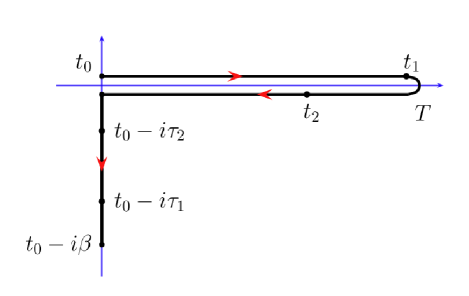
where is the operator in the Heisenberg picture and , for , is the time-ordered evolution operator of the system. We further wrote as an evolution operator in imaginary time. If we read the time arguments in Eq.(4) from right to left we see that they follow a time-contour as displayed in Fig.1. This contour is also known as the Keldysh contour Keldysh (1964); van Leeuwen et al. (2006). A more detailed inspection of Eq.(4) then shows that the expectation value can also be written as a contour-ordered product van Leeuwen et al. (2006); Stefanucci and Almbladh (2004); Wagner (1996); Dahlen et al. (2006a, b).
The one-particle Green function is then defined as a countour-ordered product of a creation and an annihilation operator
| (5) |
where denotes the time-ordering operator on the contour and where we used the compact notation and . If we consider the Green function at time and use the cyclic property of the trace, we find that Dahlen et al. (2006a). Hence, the Green function defined in Eq. (5) obeys the boundary conditions
| (6) | |||||
| (7) |
The Green function satisfies the equation of motion
| (8) |
as well as a corresponding adjoint equation Danielewicz (1984); Dahlen et al. (2006a). In Eq.(8) the time-integration is carried out along the contour . The self-energy incorporates the effects of exchange and correlation in many-particle systems and is a functional of the Green function that can be defined diagrammatically Danielewicz (1984); Fetter and Walecka (1971). The Green function can be written as
| (9) |
where is a step function generalized to arguments on the contour i.e. with if is later on the contour than and zero otherwise Danielewicz (1984). The greater and lesser components and respectively, have the explicit form
| (10) | |||||
| (11) |
When one of the arguments is on the vertical track of the contour, we adopt the notation Stefanucci and Almbladh (2004)
| (12) | |||||
| (13) |
Finally, for the case when both time arguments are on the imaginary track of the contour, we have the so-called Matsubara Green function Fetter and Walecka (1971)
| (14) |
which is a well-known object from the equilibrium theory. The factor in the definition of Eq.(14) is a convention which ensures that is a real function. The self-energy has a similar general structure as the Green function
| (15) |
The main difference with Eq.(9) is the appearance of the term which is proportional to a contour delta function in the time coordinates Danielewicz (1984). This term has the explicit form
| (16) |
where
| (17) | |||||
The structure of this self-energy is that of the Hartree-Fock (HF) approximation. However, in general we will evaluate this expression for Green functions obtained beyond HF level (see section III). Using the form of the self-energy of Eq.(15) the contour integrations can be readily carried out Danielewicz (1984); van Leeuwen et al. (2006) and we find separate equations for the different Green functions and . To display their temporal structure more clearly we surpress the spatial indices of the Green functions and self-energies. Alternatively, these quantities may be regarded as matrices Dahlen and van Leeuwen (2007). On the imaginary track of the contour we obtain
| (18) |
where the Green function and the self-energy are functions of the time-differences only, i.e. and , since the Hamiltonian is time-independent (and equal to ) on the imaginary track. Equation (18), which determines the Green function of the equilibrium system, has been treated in detail in references Dahlen and van Leeuwen (2005); Stan et al. (2009). For the other Green functions we obtain
| (19) | |||||
| (20) | |||||
| (21) | |||||
| (22) |
where and is given by Eq.(17). The retarded and advanced functions for and are defined according to
| (23) |
with replaced by and respectively. The so-called collision terms and have the form
| (24) | |||||
| (25) | |||||
| (26) | |||||
| (27) | |||||
These equations are readily derived using the conversion table of Ref. van Leeuwen et al. (2006). From the symmetry relations
| (28) | |||||
| (29) |
it follows that we only need to calculate and for and and for . These equations imply that . We further have
| (30) | |||||
| (31) |
The symmetry relations (28) and (30) for the Green function follow directly from
its definition, whereas
the symmetry relations (29) and (31) for the self-energy
follow from Eqs.(3.19) and (3.20) of Ref. Danielewicz (1984).
Another consequence of equations (30) and (31) is that ,
which means that in practice it is sufficient to calculate only and .
Eqs.(19) to (22) are known as the Kadanoff-Baym
equations Kadanoff and Baym (1962); Danielewicz (1984).
Once the Matsubara Green function is obtained from Eq.(18),
the Green functions can be calculated by time propagation.
Their initial conditions are
| (32) | |||||
| (33) | |||||
| (34) | |||||
| (35) |
The KB equations, together with the initial conditions, completely determine the Green functions for all times once a choice for the self-energy has been made. The form of the self-energy will be the topic of the next section.
III Self-energy approximations
In the applications of the KB equations it is possible to guarantee that the macroscopic conservation laws, such as those of particle, momentum and energy conservation, are obeyed. Baym Baym (1962) has shown that this is the case whenever the self-energy is obtained from a functional , such that
| (36) |
Such approximations to the self-energy are called conserving
or -derivable approximations.
Well-known conserving approximations are the Hartree-Fock, the second Born Kadanoff and Baym (1962), the Hedin (1965),
and the -matrix Kadanoff and Baym (1962) approximation.
In our work we implemented the first three of these.
The second Born approximation –
This
approximation for the self-energy
consists of the two diagrams to second order in the two-particle interaction Kadanoff and Baym (1962); Baym and Kadanoff (1961)
| (37) |
where is the HF part of the self energy of Eq.(16) and is the sum of the two terms
| (39) | |||||
where . These terms are usually referred to as the second-order direct and exchange terms. This approximation to the self-energy has been discussed in detail for the equilibrium case in Ref. Dahlen and van Leeuwen (2005). For the nonequilibrium case we need to calculate the various components . These are explicitly given by
| (41) | |||||
for the direct diagram, and
| (43) | |||||
for the second-order exchange diagram.
These expressions follow immediately from Eqs.(39) and (39)
with help of the conversion table of Ref. van Leeuwen et al. (2006).
The approximation –
In the approximation the exchange-correlation part of the self-energy
is given as a product of the Green function with a
dynamically screened
interaction Hedin (1965) .
The screened interaction satisfies the equation
| (44) |
Here, is the bare Coulomb interaction, and
| (45) |
is the irreducible polarization Hedin (1965). However, since the first term in Eq.(44) is singular in time (proportional to a delta function) it is convenient, for numerical purposes, to define its time-nonlocal part Stan et al. (2009). From Eq.(44) it follows that
| (46) | |||||
In terms of , the self-energy has the form Hedin (1965)
| (47) |
The part represents the correlation part of the self-energy and has the components
| (48) | |||||
| (49) |
From the fact that has the same symmetries as the contour-ordered density response function Hedin (1965) , where is the density operator, it follows that
| (50) | |||||
| (51) |
In the following, we will again surpress the spatial coordinates in order to display the temporal structure of the equations more clearly. From the symmetry relations (50), (51), (48) and (49), and the fact that we only need for and for , it follows that we only need to calculate , and for . The latter obey the equations:
| (52) | |||||
| (53) |
where
| (54) | |||||
| (55) |
and where the terms and are given by
| (56) | |||||
| (57) | |||||
with the retarded and advanced quantities defined as in Eq.(23). The initial conditions for and are
| (58) | |||||
| (59) |
where is the Matsubara interaction discussed in detail in Ref. Stan et al. (2009).
IV Time-propagation of the Kadanoff-Baym equations
In the following, we will describe the time-propagation method which we employed to
solve the KB equations.
This method can be applied to general Hamiltonians
containing one- and two-body interactions,
and is further independent of the explicit form of the self-energy.
The time-propagation method is applied to the KB equations in matrix form. This matrix form is obtained by expressing the Green function in terms of a set of basis functions , which we choose to be Hartree-Fock orbitals Dahlen and van Leeuwen (2005, 2007); Stan et al. (2009)
| (60) |
When Eq.(60) is inserted in the expressions for the
self-energy we obtain a basis set representation of the self-energy
involving the matrices and the two-electron integrals
which are given as integrals of orbital products with the two-body interaction .
All the quantities therefore become time-dependent matrices and all
products are to be interpreted as matrix products.
We will, however, surpress all matrix indices
to display the temporal structure of the equations more clearly.
Explicit expressions of the matrix form of the second Born and self-energy
are given in Refs.Dahlen and van Leeuwen (2005, 2007); Stan et al. (2009).
We start by discussing the time-propagation of and .
Due to the symmetry relations Eq.(28) and (29)
we only need to calculate for and
for .
From Eqs.(19) and (20) it then follows that
must be time-stepped in the first time-argument and
in the second one. We thus need to calculate
and for a
small time step ,
from the knowledge of for .
The symmetry relations (28) then immediately provide us
with and as well.
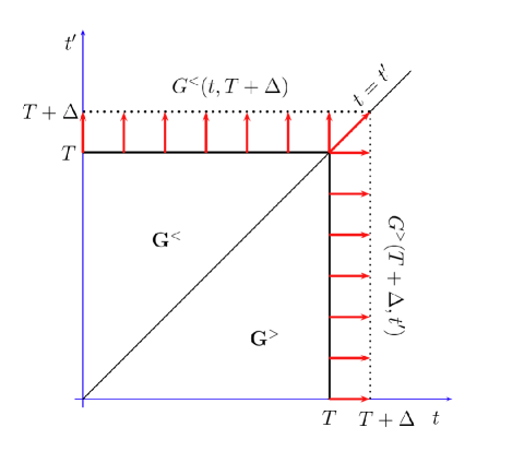
The time-stepping procedure is illustrated in Fig.2
that displays the -plane, in which at a given time all the quantities
inside the square with sides equal to , are known.
The time-step
corresponds to a shift of the upper side of the time square with
i.e. a shift from the solid to the dotted line in Fig.2.
Similarly the time-step corresponds
to a shift of the righthand side of the time square with .
We further need to make a step along the
time diagonal .
The propagation of and
requires a time-step in the real time coordinate for fixed imaginary time points .
Note that the righthand sides of Eqs.(19) to (22)
depend on the Green functions at the times , which are not
known at time .
We therefore carry out the time-step twice.
After taking the time step for the first time, we recalculate the righthand sides of Eqs.(19) to (22)
and repeat the time-step using an average of the old and new collision and HF terms.
Since the term in Eqs.(19) to (22)
can attain large values, it is favorable to eliminate this term from the time-stepping equations.
For each time-step we therefore absorb the term in a time-evolution
operator of the form
| (61) |
where , where is the one-body part of the Hamiltonian of Eq.(2). The one-body Hamiltonian is explicitly known as a function of time and can be evaluated at half the time-step. The term is only known at time and will be recalculated in the repeated time-step. In terms of the operator of (61) we define new Green function matrices , as
| (62) | |||||
| (63) | |||||
| (64) |
We can now transform Eqs.(19) to (22) into equations for . For instance, satisfies the equation
| (65) | |||||
Since for times , we can neglect for these times the first term on the right hand side of Eq.(65). We then find
| (66) | |||||
where is defined as
| (67) |
Similarly for , which is propagated using Eq.(20), we find the equation
| (68) | |||||
For time-stepping along the time-diagonal we use
| (69) | |||||
which follows directly from a combination of the equations for of Eqs.(19) and (20). The corresponding equation for on the time diagonal then becomes
| (70) | |||||
From this equation we then obtain
| (71) | |||||
where we defined . By using the operator expansion
| (72) | |||||
it follows that
| (73) |
where
| (74) |
and . If we insert Eq.(73) into Eq.(71) we finally obtain
| (75) |
We found that keeping terms for only, yields sufficient accuracy. We now consider the time propagation for the mixed real and imaginary time Green functions. For we have the equation
| (76) | |||||
This yields, similarly as in Eq.(66) and (68)
| (77) | |||||
Finally, for we have
| (78) | |||||
The Eqs. (66), (68), (71),
(77) and (78) form the basis of the time-stepping algorithm.
At each time-step, it requires the construction of the step operators and
and therefore the diagonalization of for every time-step.
As mentioned before, the righthand sides of Eqs.(19) to (22)
depend on the Green functions at the times which are not
known at time . We therefore carry out the time-step twice.
The procedure is as follows:
(1) The collision integrals and at time are calculated from the Green functions
for times .
(2) A step in the Green function is taken
according to Eqs.(66), (68), (71), (77)
and (78).
(3) New collision integrals
and are calculated by inserting the new Green functions
for times into Eqs.(24) to (27).
(4) The values of the collision integrals and the Hartree-Fock self-energy are approximated
by and
where and are the collision terms calculated under points (1) and (3).
(5) The Green function is then propagated from
using the average values and
in Eqs.(66), (68), (71), (77)
and (78).
This concludes the general time-stepping procedure for the Green functions.
We finally consider the calculation of and from Eqs. (52) and (53).
As a consequence of the symmetry relation (50), we only need to calculate for .
In a time step from to we need to calculate for
from the known values of for .
The first term on the righthand side of Eq.(52) can be calculated
directly from and . However, the last term
of Eq.(52) depends on the, still undetermined, values . We therefore employ an
iterative scheme. As a first guess for we take
for and .
We therefore use the values of on the known sides of the time square at
time (solid lines in Fig.2) as initial guesses for the stepped sides
(dotted lines in Fig.2) at .
As an initial guess for the value of at the new diagonal point ,
we take the value at the previous diagonal point .
We then calculate the quantity for
and obtain a new value for from Eq.(52).
This value is then inserted back into the righthand side of Eq.(52)
and the process is repeated until convergence is reached.
Similarly we initialize
and solve Eq.(53) in the same manner as for .
This concludes our derivation of the time-stepping algorithm of the KB equations.
The propagation method described here has been used in two recent Letters Dahlen and van Leeuwen (2007); Myöhanen et al. (2008)
where also values for the numerical parameters are given. It is clear that the choice
of these parameters depends strongly on the type of system considered, and on the strength of
the applied external fields.
V Summary and conclusions
We presented a detailed account of the KB equations and discussed in detail their structure, initial conditions and symmetries. We developed an algorithm for the time-propagation of the KB equations in which the symmetry relations for the Green functions were used to reduce the set equations that needed to be solved. In two recent Letters Dahlen and van Leeuwen (2007); Myöhanen et al. (2008) we applied the method to the case of atoms and molecules in external time-dependent fields and to the case of transient transport dynamics of double quantum dots. We therefore conclude that time-propagation of the KB equations can be used as a practical method to calculate the nonequilibrium properties of a wide variety of many-body quantum systems, ranging from atoms and molecules to quantum dots and quantum wells. Moreover, the present work can be readily extended to other Green function formalisms, such as the Nambu formalism Nambu (1960); Schrieffer (1988) for superconducting systems. Also future extension to bosonic systems is straightforward. Work along these lines is in progress.
References
- Cuniberti et al. (2005) G. Cuniberti, G. Fagas, and K. Richter, eds., Introducing Molecular Electronics, vol. 680 (Springer, New York, 2005).
- Kato et al. (2003) T. H. T. Kato, T. Aoki, T. Ando, A. Fukuda, and S.-S. Seomun, Phys. Rev. Lett. 91, 226804 (2003).
- Elzerman et al. (2003) J. M. Elzerman, R. Hanson, L. H. W. van Beveren, B. Witkamp, L. M. K. Vandersypen, and L. P. Kouwenhoven, Nature 430, 431 (2003).
- Shah (1999) J. Shah, ed., Ultrafast Spectroscopy of Semiconductors and Semiconductor Nanostructures (Springer, Berlin, 1999).
- Merano et al. (2007) M. Merano, S. Sonderegger, A. Crottini, S. Collin, P. Renucci, E. Pelucchi, A. Malko, M. Baier, E. Kapon, B. Deveaud, et al., Nature 438, 479 (2007).
- Baym (1962) G. Baym, Phys. Rev. 127, 1391 (1962).
- Dahlen and van Leeuwen (2007) N. E. Dahlen and R. van Leeuwen, Phys. Rev. Lett. 98, 153004 (2007).
- Kadanoff and Baym (1962) L. P. Kadanoff and G. Baym, Quantum Statistical Mechanics (W. A. Benjamin, Inc., New York, 1962).
- Danielewicz (1984) P. Danielewicz, Ann. Phys. (N. Y.) 152, 239 (1984).
- Kwong and Bonitz (2000) N.-H. Kwong and M. Bonitz, Phys. Rev. Lett. 84, 1768 (2000).
- Myöhanen et al. (2008) P. Myöhanen, A. Stan, G. Stefanucci, and R. van Leeuwen, Europhys. Lett. 84, 67001 (2008).
- Schäfer (1996) W. Schäfer, J.Opt.Soc.Am. B13, 1291 (1996).
- Bonitz et al. (1996) M. Bonitz, D. Kremp, D. C. Scott, R. Binder, W. Kraeft, and H. S. Köhler, J.Phys.Cond.Matter 8, 6057 (1996).
- Binder et al. (1997) R. Binder, H. S. Köhler, M. Bonitz, and N. Kwong, Phys.Rev. B55, 5110 (1997).
- Dahlen and van Leeuwen (2005) N. E. Dahlen and R. van Leeuwen, J. Chem. Phys. 122, 164102 (2005).
- Stan et al. (2009) A. Stan, N. E. Dahlen, and R. van Leeuwen, J. Chem. Phys. (accepted) (2009).
- Köhler et al. (1999) H. S. Köhler, N. H. Kwong, and H. A. Yousif, Comp. Phys. Comm. 123, 123 (1999).
- Bonitz and Semkat (2006) M. Bonitz and D. Semkat, in Introduction to Computational Methods in Many-Body Physics, edited by M. Bonitz and D. Semkat (Rinton Press, Princeton, 2006), p. 171.
- Fetter and Walecka (1971) A. L. Fetter and J. D. Walecka, Quantum Theory of Many-Particle Systems (McGraw-Hill, New York, 1971).
- van Leeuwen et al. (2006) R. van Leeuwen, N. E. Dahlen, G. Stefanucci, C.-O. Almbladh, and U. von Barth, in Time-dependent Density Functional Theory, edited by M. A. L. Merques, C. A. Ullrich, F. Nogueira, A. Rubio, K. Burke, and E. K. U. Gross (Springer, Berlin Heidelberg, 2006), p. 33.
- Keldysh (1964) L. V. Keldysh, Zh. Eksp. Teor. Fiz. 47, 1515 (1964), [Sov. Phys. JETP, 20, 1018 (1965)].
- Stefanucci and Almbladh (2004) G. Stefanucci and C.-O. Almbladh, Phys. Rev. B 69, 195318 (2004).
- Wagner (1996) M. Wagner, Phys. Rev. B 44, 6104 (1996).
- Dahlen et al. (2006a) N. E. Dahlen, A. Stan, and R. van Leeuwen, J. Phys. Conf. Ser. 35, 324 (2006a).
- Dahlen et al. (2006b) N. E. Dahlen, R. van Leeuwen, and A. Stan, J. Phys. Conf. Ser. 35, 340 (2006b).
- Hedin (1965) L. Hedin, Phys. Rev. 139, A796 (1965).
- Baym and Kadanoff (1961) G. Baym and L. P. Kadanoff, Phys. Rev. 124, 287 (1961).
- Schrieffer (1988) J. R. Schrieffer, Theory of Superconductivity (Addison-Wesley, 1988).
- Nambu (1960) Y. Nambu, Phys.Rev. 117, 648 (1960).