On simultaneous hitting of membranes by two skew Brownian motions

Abstract.

We consider two depending Wiener processes which have membranes at zero with different permeability coefficients. Starting from different points, the processes almost surely do not meet at any fixed point except that where membranes are situated. The necessary and sufficient conditions for the meeting of the processes are found. It is shown that the probability of meeting is equal to zero or one.

Introduction

Let $\left(w_{1}(t)),(w_{2}(t)\right)_{t\geq 0}$ be a two-dimensional Wiener process with the correlation matrix

$$B=\begin{pmatrix}1&\alpha\\ \alpha&1\end{pmatrix}t,$$

where $\alpha\in(-1,1)$ is some constant.

Consider the equations

(1) $$x_{1}(t) = x_{1}(0)+w_{1}(t)+\varkappa_{1}L_{x_{1}}^{0}(t),$$

(2) $$x_{2}(t) = x_{2}(0)+w_{2}(t)+\varkappa_{2}L_{x_{2}}^{0}(t),$$

where $\{\varkappa_{1},\varkappa_{2}\}\in[-1,1]$ are constants,

$$L_{x_{i}}^{0}(t)=\lim_{\varepsilon\downarrow 0}\frac{1}{2\varepsilon}\int_{0}^{t}\mathds{1}_{[-\varepsilon,\varepsilon]}(x_{i}(s))ds,\ i=1,2,$$

is a local time of the process $(x_{i}(t))_{t\geq 0}$ at zero. As is known (cf. [1]), each of equations (1), (2) has a unique solution, which is a skew Brownian motion. Here $\varkappa_{1}$ and $\varkappa_{2}$ can be treated as coefficients of permeability. If $\varkappa_{1}=1$, the part of the process $(x_{1}(t))_{t\geq 0}$ on the positive semi-axis is a Wiener process with reflection at $0$; if $\varkappa_{1}=-1$, then the part of the process $(x_{1}(t))_{t\geq 0}$ on the negative semi-axis is a Wiener process with reflection at $0$; if $\varkappa_{1}\in(-1,1)$, then there is a semipermeable membrane at $0$.

The aim of the paper is to calculate the probability of simultaneous hitting of the membranes by the processes $(x_{1}(t))_{t\geq 0}$ and $(x_{2}(t))_{t\geq 0}$. This probability turns out to be determined by the sign of an expression involving $\varkappa_{1},\varkappa_{2},\alpha.$ Besides it is equal to zero or one.

The case of $\alpha=1$ is studed in [2], [3]. In [2] it is proved that if $\{\varkappa_{1},\varkappa_{2}\}\in[-1,1]\setminus\{0\}$ then the processes $(x_{1}(t))_{t\geq 0}$ and $(x_{2}(t))_{t\geq 0}$ meet in finite time with probability 1. In [3] it is obtained that if $x_{1}(0)=x_{2}(0)=0,$ $0<\varkappa_{1}<\varkappa_{2}<1,$ and $\varkappa_{1}>\varkappa_{2}/(1+2\varkappa_{2}),$ then for each $t_{0}>0$ there exists $t>t_{0}$ such that $x_{1}(t)=x_{2}(t).$ The problem of simultaneous hitting of the sphere by two Brownian motion with normal reflection on the sphere is treated in [4] (two-dimensional case) and [5].

If there are no membranes, i.e. $\varkappa_{1}=\varkappa_{2}=0,\alpha\neq 1$, then the process $x(t)=\left(x_{1}(t),x_{2}(t)\right),t\geq 0,$ is a two-dimensional Wiener process. It reaches any fixed point $x_{0}\in\mathbb{R}^{2},$ $x_{0}\neq x(0),$ with probability 0. In particular this implies that the process $(x(t))_{t\geq 0}$ almost surely does not hit any fixed point except the points at which at least one membrane is situated.

There is one more problem of stochastic analysis where the study of simultaneous membrane visitation arises naturally. Assume that we are attending to construct a flow generated by stochastic differential equation with a semipermeable membrane located on a hyperplane [7]. Note that there is no general results on existence and uniqueness of a strong solution to such equations in multidimensional space. In order to construct the flow on some probability space it is sufficient to construct a sequence of consistent (weak) $n$-point motions [8]. One-point motion can be constructed by N.Portenko’s methods [7]. There are no general results on weak uniqueness for two-point motion, when both points start from the membrane. However, if the simultaneous visitation the membrane has a probability 0, then there is a hope to construct $n$-point motion using localization at the neighborhood of membrane. Unfortunately, the results of the article show that synchronous hitting the membrane is quite natural.

1. Transformation of the processes

The pair of the processes $(x_{1}(t),x_{2}(t))_{t\geq 0}$ can be thought off as a new process in Euclidean space $\mathbb{R}^{2}$ with membranes on the straight-lines $S_{1}=\{x_{2}=0\}$ $S_{2}=\{x_{1}=0\}$. The membranes act in the normal direction $\nu_{1}=(0,1)$ and $\nu_{2}=(1,0)$ to $S_{1}$ and $S_{2}$ respectively.

Let us make a coordinate transformation defined by the linear operator

$$A=B^{-1/2}=\frac{1}{c}\begin{pmatrix}a&b\\ b&a\end{pmatrix},$$

where

$$a = \sqrt{1-\alpha}+\sqrt{1+\alpha},$$

$$b = \sqrt{1-\alpha}-\sqrt{1+\alpha},$$

$$c = 2\sqrt{1-\alpha^{2}}.$$

As a result we get a new process $(\tilde{x}_{1}(t),\tilde{x}_{2}(t))_{t\geq 0}.$ From (1), (2) we see that its trajectories are solutions of the following equations

(3) $$\tilde{x}_{1}(t) = \tilde{x}_{1}(0)+\tilde{w}_{1}(t)+\varkappa_{1}\frac{a}{c}L_{x_{1}}^{0}(t)+\varkappa_{2}\frac{b}{c}L_{x_{2}}^{0}(t),$$

(4) $$\tilde{x}_{2}(t) = \tilde{x}_{2}(0)+\tilde{w}_{2}(t)+\varkappa_{1}\frac{b}{c}L_{x_{1}}^{0}(t)+\varkappa_{2}\frac{a}{c}L_{x_{2}}^{0}(t),$$

where $\tilde{w}_{1}(t)={a}/cw_{1}(t)+b/cw_{2}(t),\ \tilde{w}_{2}(t)={b}/cw_{1}(t)+a/cw_{2}(t),\ t\geq 0.$ It is easily seen that the correlation matrix of the vector $(\tilde{w}_{1}(t),\tilde{w}_{2}(t))$ is as follows

$$\begin{pmatrix}1&0\\ 0&1\end{pmatrix}t.$$

This yields that $(\tilde{w}_{1}(t))_{t\geq 0}$ and $(\tilde{w}_{2}(t))_{t\geq 0}$ are independent Wiener processes.

Denote by $S_{1}^{\,\prime}$ and $S_{2}^{\,\prime}$ the images of $S_{1}$ and $S_{2}$ under the transformation defined by the matrix $A$. Then equations (3), (4) can be rewritten in the form

(5) $$\tilde{x}_{1}(t) = \tilde{x}_{1}(0)+\tilde{w}_{1}(t)+\varkappa_{1}\frac{a}{c}L_{\tilde{x}}^{S_{1}^{\,\prime}}(t)+\varkappa_{2}\frac{b}{c}L_{\tilde{x}}^{S_{2}^{\,\prime}}(t),$$

(6) $$\tilde{x}_{2}(t) = \tilde{x}_{2}(0)+\tilde{w}_{2}(t)+\varkappa_{1}\frac{b}{c}L_{\tilde{x}}^{S_{1}^{\,\prime}}(t)+\varkappa_{2}\frac{a}{c}L_{\tilde{x}}^{S_{2}^{\,\prime}}(t),$$

where $L_{\tilde{x}}^{S_{i}^{\,\prime}}$ is a symmetric local time of the process $(\tilde{x}(t))_{t\geq 0}$ on the straight-line $S_{i}^{\,\prime}$ that is

(7) $$L_{\tilde{x}}^{S_{i}^{\,\prime}}(t)=\lim_{\varepsilon\downarrow 0}\frac{1}{2\varepsilon}\int_{0}^{t}\mathds{1}_{A_{\varepsilon}^{i}}(\tilde{x}(s))ds,\ i=1,2,$$

$$A_{\varepsilon}^{i}=\{x\in\mathbb{R}^{2}:\exists y\in S_{i}^{\,\prime},s\in[-1,1]\mbox{ such that }x=y+\varepsilon s\nu_{i}^{\,\prime}\},$$

$\nu_{i}^{\,\prime},\ i=1,2,$ is the image of $\nu_{i}$ under the transformation defined by the matrix $A$.

2. On hitting of zero by the Wiener process on the plane with membranes on rays with a common endpoint

A Wiener process in $\mathbb{R}^{2}$ with membranes on rays $c_{1},\dots,\ c_{n}$ having a common endpoint was investigated in [6]. Let $(r,\varphi),r\geq 0,\varphi\in[0,2\pi),$ be polar coordinates in $\mathbb{R}^{2}$ and let

$$c_{k}=\{(r,\varphi):r\geq 0,\ \varphi=\varphi_{k}\},$$

where $0\leq\varphi_{1}<\dots<\varphi_{n}<2\pi$. Put $\varphi_{n+1}=\varphi_{n},$ $\xi_{k}=\varphi_{k+1}-\varphi_{k},k=1,2,\dots,n$, and $\xi_{0}=\xi_{n}$.

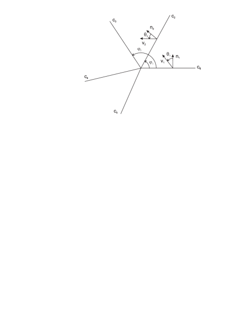
Figure 1.

Denote by $n_{k},k=1,\dots,n,$ the unit vector normal to $c_{k}$ that points anticlockwise and let $v_{k}$ be a vector in $\mathbb{R}^{2}$ such that $(v_{k},n_{k})=1$. The angle between $n_{k}$ and $v_{k}$ denoted by $\theta_{k}\in(-\frac{\pi}{2},\frac{\pi}{2})$ is referred to as a positive if and only if $v_{k}$ points towards the origin. Let $\gamma_{k},|\gamma_{k}|\leq 1,\ k=1,\dots,n,$ be the membrane permeability coefficients. The case of $n=5,\theta_{1}>0,\theta_{2}>0$ is shown in Fig. 1.

It was proved in [6] that there exists a unique strong solution to the equation

(8) $$dx(t)=dw(t)+\sum_{k=1}^{n}\gamma_{k}v_{k}dL_{x}^{c_{k}}(t)$$

in $\mathbb{R}^{2}$ with the initial condition $x(0)=x^{0},\ x^{0}\in\mathbb{R}^{2},$ up to the time $\zeta,$ where $\zeta=+\infty$ or $x(\zeta-)=0.$

Further on we make use of the following Proposition on hitting $0$ or $\infty$ by the process $(\tilde{x}(t))_{t\geq 0}$ (cf. [6]).

Proposition 1.

Let $\gamma_{k}\in[-1,1],\ k=1,\dots,n$, and let the Markov chain with the state-space $\{1,\dots,n\}$ and the transition matrix

$$\begin{pmatrix}0&\tilde{p}_{1}&0&0&\ldots&0&0&0&\tilde{q}_{1}\\ \tilde{q}_{2}&0&\tilde{p}_{2}&0&\ldots&0&0&0&0\\ [3]{9}\\ 0&0&0&0&\ldots&0&\tilde{q}_{n-1}&0&\tilde{p}_{n-1}\\ \tilde{p}_{n}&0&0&0&\ldots&0&0&\tilde{q}_{n}&0\end{pmatrix},$$

where

(9) $$\tilde{p}_{k} = \frac{(1+\gamma_{k})\xi_{k-1}}{(\xi_{k-1}+\xi_{k})+\gamma_{k}(\xi_{k-1}-\xi_{k})},$$

(10) $$\tilde{q}_{k} = \frac{(1-\gamma_{k})\xi_{k}}{(\xi_{k-1}+\xi_{k})+\gamma_{k}(\xi_{k-1}-\xi_{k})},$$

has a unique invariant distribution $(\pi_{k})_{k=1}^{n}$.

Then if $\sum_{k=1}^{n}\gamma_{k}\pi_{k}\frac{\xi_{k-1}\xi_{k}}{{(\xi_{k-1}+\xi_{k})+\gamma_{k}(\xi_{k-1}-\xi_{k})}}\tan\theta_{k}>0$ then the process $(\tilde{x}(t))_{t\geq 0}$ hits the origin almost surely;
if $\sum_{k=1}^{n}\gamma_{k}\pi_{k}\frac{\xi_{k-1}\xi_{k}}{{(\xi_{k-1}+\xi_{k})+\gamma_{k}(\xi_{k-1}-\xi_{k})}}\tan\theta_{k}\leq 0$ then the process $(\tilde{x}(t))_{t\geq 0}$ does not hit the origin a.s.

3. The main result

Let us formulate our problem in terms of the previous Section. Let $c_{1},c_{2},c_{3},c_{4}$ be the images of the rays $[0,\infty)\times\{0\},$ $\{0\}\times[0,\infty)$, $(-\infty,0]\times\{0\}$, $\{0\}\times(-\infty,0]$ under the linear transformation $A$. The images of $\nu_{1}=(0,1)$ and $\nu_{2}=(1,0)$ are the vectors $\nu_{1}^{\prime}=(a/c,b/c)$ and $\nu_{2}^{\,\prime}=(b/c,a/c)$. Denote by $\xi$ the angle between them. Then

$$\cos\xi=\frac{(\nu_{1}^{\,\prime},\nu_{2}^{\,\prime})}{|\nu_{1}^{\,\prime}|\cdot|\nu_{2}^{\,\prime}|}=\frac{2ab}{a^{2}+b^{2}}=-\alpha.$$

The case of $\alpha<0$ is shown in Fig. 2.

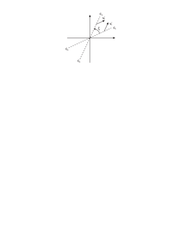
Figure 2.

Put $\xi_{1}=\xi_{3}=\xi,\ \xi_{2}=\xi_{4}=\pi-\xi$, $\gamma_{1}=-\gamma_{3}=\varkappa_{1},\ \gamma_{2}=-\gamma_{4}=-\varkappa_{2}$, $v_{1}=(a/c,b/c)$, $v_{2}=(-b/c,-a/c)$, $v_{3}=(-a/c,-b/c)$, $v_{4}=(b/c,a/c),$ $\theta_{1}=\theta_{3}=\xi-\pi/2,$ $\theta_{2}=\theta_{4}=\pi/2-\xi$. It is easy to check that $(v_{i},n_{i})=1,i=1,2,3,4,$ where $n_{i}$ is the unit normal vector to $c_{i}$ that points anticlockwise. Indeed,

$$(v_{i},n_{i})=\frac{\sqrt{a^{2}+b^{2}}}{c}\cos{(\pi/2-\xi)}=\frac{2}{2\sqrt{1-\alpha^{2}}}\sqrt{1-\alpha^{2}}=1,\\ i=1,2,3,4.$$

Equations (5),(6) can be rewritten as follows

(11) $$\tilde{x}(t)=\tilde{x}(0)+\tilde{w}(t)+\sum_{i=1}^{4}\gamma_{i}v_{i}L_{\tilde{x}}^{c_{i}}(t),\ t\leq\zeta,$$

where $\tilde{x}(t)=(\tilde{x}_{1}(t),\tilde{x}_{2}(t)),\tilde{w}(t)=(\tilde{w}_{1}(t),\tilde{w}_{2}(t)),\ \zeta$ is the first hitting time of 0 by the process $(\tilde{x}(t))_{t\geq 0}$. So (11) coincides with (8).

Now we calculate the expression from Proposition for $n=4$:

$$S=\sum_{k=1}^{4}\gamma_{k}\pi_{k}\frac{\xi_{k-1}\xi_{k}}{{(\xi_{k-1}+\xi_{k})+\gamma_{k}(\xi_{k-1}-\xi_{k})}}\tan\theta_{k}.$$

Let $\{\varkappa_{1},\varkappa_{2}\}\in(-1,1)\setminus\{0\}$. The invariant distribution $(\pi_{i})_{i=1}^{4}$ can be obtained directly. But we make use of formula (29) from [6]. We have

$$\pi_{1}=\frac{\tilde{q}_{2}\tilde{q}_{3}\tilde{q}_{4}}{\tilde{p}_{1}\tilde{q}_{3}\tilde{q}_{4}+\tilde{p}_{1}\tilde{p}_{2}\tilde{q}_{4}+\tilde{p}_{1}\tilde{p}_{2}\tilde{p}_{3}+\tilde{q}_{2}\tilde{q}_{3}\tilde{q}_{4}}.$$

Taking into account (9),(10) we get

$$\pi_{1} = \frac{(1-\gamma_{2})\left((1+\gamma_{1})(\pi-\xi)+(1-\gamma_{1})\xi\right)}{D},$$

$$\pi_{2} = \frac{(1+\gamma_{1})\left((1-\gamma_{2})(\pi-\xi)+(1+\gamma_{2})\xi\right)}{D},$$

$$\pi_{3} = \frac{(1+\gamma_{2})\left((1-\gamma_{1})(\pi-\xi)+(1+\gamma_{1})\xi\right)}{D},$$

$$\pi_{4} = \frac{(1-\gamma_{1})\left((1+\gamma_{2})(\pi-\xi)+(1-\gamma_{2})\xi\right)}{D},$$

where $D=2\left[(1+\gamma_{1}\gamma_{2})\xi+(1-\gamma_{1}\gamma_{2})(\pi-\xi)\right]>0.$ Then

$$S=2\frac{\xi(\pi-\xi)}{D}(-\varkappa_{1}\varkappa_{2}\cot\xi).$$

The condition $\xi\in(0,\pi)$ yields $\cot\xi=-\frac{\alpha}{\sqrt{1-\alpha^{2}}}.$ Consequently $S>0$ if and only if $\varkappa_{1}\varkappa_{2}\alpha>0.$

It is obvious that the processes $(x_{1}(t))_{t\geq 0}$ and $(x_{2}(t))_{t\geq 0}$ meet in zero when and only when $(\tilde{x}(t))_{t\geq 0}$ hits zero.

If $\varkappa_{1}=\varkappa_{2}=1$ then there exists a unique invariant distribution $\pi_{1}=\pi_{2}=1/2,\ \pi_{3}=\pi_{4}=0$. It is easily to see that now $S>0$ if and only if $\alpha>0.$

Finally, let $\varkappa_{1}=1,\ \varkappa_{2}\in(-1,1)\setminus\{0\}.$ Then the invariant distribution is of the form $\pi_{1}=\tilde{p}_{2}/2,\ \pi_{2}=1/2,\ \pi_{3}=\tilde{q}_{2}/2,\ \pi_{4}=0.$ We get that $S>0$ if and only if $\varkappa_{2}\alpha>0.$

The other cases when the modulus of at least one permeability coefficient is equal to 1 can be treated analogously.

Now let $\varkappa_{1}=0$. Then the unique invariant distribution is as follows $\pi_{1}=\pi_{3}=0,$ $\pi_{2}=\pi_{4}=1/2.$ It is easy to see that in this case $S=0$. Analogously, $S=0$ if $\varkappa_{2}=0$.

Thus we have proved the following statement.

Theorem 1.

Let $(x_{1}(0),x_{2}(0))\in\mathbb{R}^{2}\setminus\{(0,0)\},\ \{\varkappa_{1},\varkappa_{2}\}\subset[-1,1]$, $\alpha\in(-1,1)$. Then

$$1)\ \mathds{P}\{\exists\ t_{0}<\infty:x_{1}(t_{0})=x_{2}(t_{0})=0\}=1\ \hbox{if }\ \varkappa_{1}\varkappa_{2}\alpha>0,$$

$$2)\ \mathds{P}\{\exists\ t_{0}<\infty:x_{1}(t_{0})=x_{2}(t_{0})=0\}=0\ \hbox{if }\ \varkappa_{1}\varkappa_{2}\alpha\leq 0.$$

Remark 1.

The conditions of processes meeting obtained in Theorem for $\alpha\in(-1,1)$ are completely different from those for $\alpha=1$ obtained in [3].

Remark 2.

As was mentioned above the process $(x(t))_{t\geq 0}$ almost surely does not hit any fixed point except the points in which at least one membrane is situated. It follows from statement 2) of Theorem that the process almost surely does not hit any fixed point in which exactly one membrane is situated.

References

• [1] Harrison J.M., Shepp L.A., On skew brownian motion, Ann. Probab., 9, 1981, pp. 309–313.
• [2] Barlow M., Burdzy K., Kaspi H., Mandelbaum A.. Coalescence of skew Brownian motion, Seminaire de Probabilites XXXV. Lecture Notes in Math., 1755, 2001, pp. 202–205.
• [3] Burdzy K., Chen Z.Q., Local time flow related to skew brownian motion, Ann. Probab, 29, 2001, N 4, pp.1693 – 1715.
• [4] Cranston M., Le Jan Y., Simultaneous boundary hitting for two point reflecting Brownian motion, LN in Math. 1372, 1989, Springer-Verlag, pp. 234 – 238.
• [5] Sheu S.S. Noncoalescence of Brownian motion reflecting on a sphere, Stoch. Anal. Applic., 19(4), 2001, pp. 545-554.
• [6] Aryasova O. V., Pilipenko A. Yu., On Brownian motion on the plane with membranes on rays with a common endpoint, Random Oper. Stoch. Equ., 2009, N 2, pp. 137–156.
• [7] Portenko N.I. Generalized diffusion processes, AMS Bookstore, 1990, 180p.
• [8] Darling R.W.R. Constructing nonhomeomorphic stochastic flows, Memoirs of AMS., 79, 1987, N 376, pp. 1–97.