Dynamics and energy landscape in a tetrahedral network glass-former: Direct comparison with models of fragile liquids

Abstract

We report Molecular Dynamics simulations for a new model of tetrahedral network glass-former, based on short-range, spherical potentials. Despite the simplicity of the forcefield employed, our model reproduces some essential physical properties of silica, an archetypal network-forming material. Structural and dynamical properties, including dynamic heterogeneities and the nature of local rearrangements, are investigated in detail and a direct comparison with models of close-packed, fragile glass-formers is performed. The outcome of this comparison is rationalized in terms of the properties of the Potential Energy Surface, focusing on the unstable modes of the stationary points. Our results indicate that the weak degree of dynamic heterogeneity observed in network glass-formers may be attributed to an excess of localized unstable modes, associated to elementary dynamical events such as bond breaking and reformation. On the contrary, the more fragile Lennard-Jones mixtures are characterized by a larger fraction of extended unstable modes, which lead to a more cooperative and heterogeneous dynamics.

1 Introduction

Network-forming amorphous materials are of great interest for technological applications, as well as of fundamental importance for the theoretical understanding of the glass transition. At a microscopic scale, the structure of network glass-formers, in both the amorphous and highly viscous regime, is characterized by strong chemical ordering and atomic arrangements that usually form an open tetrahedral network. Upon cooling from high temperature, transport coefficients and structural relaxation times $\tau$ of network liquids display a mild temperature dependence, often describable by the Arrhenius law $\tau\approx\tau_{\infty}\exp(E/T)$. Network glass-formers are thus “strong” in the Angell’s classification scheme [1]. In contrast, other classes of glass-formers, including molecular, polymeric, and bulk metallic liquids, show super-Arrhenius temperature dependence of $\tau$, i.e., “fragile” behaviour.

Ever since the introduction of the Angell’s classification, the nature of the distinction between fragile and strong liquids has been highly debated. While the degree of fragility of a liquid correlates quantitatively with other macroscopic physical properties, the existence of qualitative differences between strong and fragile systems has been questioned. Evidence of a “fragile-to-strong” crossover in simulated network liquid [2] and numerical investigations of dynamic heterogeneities in model glass-formers [3] suggest that network liquids may just be an extreme case of the class of fragile systems [4]. In contrast, theoretical work on kinetically constrained models of glassy dynamics [5] indicates that strong behaviour may arise from the different nature of dynamical constraints. Moreover, the energy landscape description of supercooled liquids [6, 7] shows that the organization and connectivity of stationary points in the Potential Energy Surface (PES) may be qualitatively different in fragile and strong glass-formers. In this two latter scenarios, fragile and strong liquids would thus belong to different “universality classes” of glass-formers.

Silica is often considered as a prototypical network glass-former. In recent years, several authors have studied structural and dynamical properties of this system through numerical simulations, employing both Molecular Dynamics (MD) and Monte Carlo techniques. One of the most realistic and popular models of silica available for molecular simulations is the BKS model introduced by Van Beest et al [8]. In this model, the interaction between Si and O atoms is described by a long-ranged Coulombic interaction, plus a short range repulsion of the Born-Mayer type. Various physical aspects of the supercooled and glassy regime of the BKS model have been analysed, including the phase diagram [9, 10], structural [11], dynamical [12, 13, 3, 4], and vibrational [14, 15, 16] properties. Investigations of the energy landscape of the BKS model have also been performed [17, 18, 19, 20]. Because of the long-ranged nature of the interactions, however, simulations using the BKS model are computationally demanding. Hence, development of simpler force-fields, capturing the basic features of network liquids, is highly desirable. Recently, in fact, simplified models for silica have been proposed, including short-ranged variants of the original BKS potential [21, 22] and primitive models based on patchy interactions [23, 24]. Other models of tetrahedral network liquids (not directly related to silica) based on spherical, patchy interactions have also been studied recently [25] and in the past [26].

In this work, we present a new model of network glass-former, based on spherical, short-ranged potentials. Our model allows efficient simulations and can be tuned to reproduce some relevant properties of amorphous silica. It does not aim at a realistic description of liquid and amorphous silica, yet it captures to a good extent the essential physics of network glass-formers. Moreover, being able to describe both network and “simple” glass-forming liquids [27, 28] with similar efficiency via the same family of interactions, we can get an unusually detailed and systematic comparison between the microscopic origins of their structural relaxation. In particular, we trace back the distinct dynamic features of network glass-formers (e.g. strong behaviour, weak dynamic heterogeneity, bond breaking and reformation processes) to the properties of the PES, contrasting our findings with the case of the more fragile, close-packed Lennard-Jones (LJ) mixtures [27, 28]. Our results emphasize the role of the unstable modes of the PES, as a key to rationalize the different dynamic behaviours of glass-forming liquids.

The paper is organized as follows: in section 2 we introduce our model of network glass-former; in section 3 we describe its structural and dynamical properties, while in section 4 we analyse the properties of the stationary points of the PES, focusing on the unstable modes. Finally, in section 5 we draw our conclusions.

2 Model

Our model of network glass-former, called NTW herein, is a binary mixture of classical particles interacting through the following forcefield

$$u_{\alpha\alpha}(r) = 4\epsilon_{\alpha\alpha}\left(\frac{\sigma_{\alpha\alpha}}{r}\right)^{12}$$ (1)

$$u_{\alpha\beta}(r) = 4\epsilon_{\alpha\beta}\left[{\left(\frac{\sigma_{\alpha\beta}}{r}\right)}^{12}-{\left(\frac{\sigma_{\alpha\beta}}{r}\right)}^{6}\right]\quad\alpha\neq\beta$$ (2)

where $\alpha$,$\beta$=1,2 are indexes of species. In the following, we will use $\sigma_{11}$, $\epsilon_{11}$ and $\sqrt{m_{1}\sigma_{11}^{2}/\epsilon_{11}}$ as reduced units of distance, energy and time respectively. Keeping an eye on silica, we identify large particles (species 1) with Si atoms and small particles (species 2) with O atoms, and we fix the number concentrations at $x_{1}=0.33$, $x_{2}=0.67$. We also use the same mass ratio of O and Si atoms: $m_{2}/m_{1}=0.57$. A smooth cut-off scheme is used to ensure continuity of $u_{\alpha\beta}(r)$ at $r=2.2\sigma_{\alpha\beta}$ up to the second derivative [29]. The size of the samples considered in this work is $N=N_{1}+N_{2}=500$. The presence of finite size effects have been checked through simulations of larger systems ($N=2048$, $8000$) and will be briefly discussed in section 3. We performed MD simulations in the NVE ensemble using quenching protocols and equilibration criteria similar to the ones of previous simulations of LJ mixtures [27, 28]. Equilibration and production runs were performed using Berendsen rescaling and velocity-Verlet algorithm, respectively. The time step $\delta t$ was varied between 0.001 (at high $T$) and 0.004 (at low $T$). The absence of major systematic aging effects was checked by comparing thermodynamic, structural, and dynamical properties in different parts of the production runs. At the lowest temperatures, simulations involved up to $3.5\times 10^{7}$ and $7\times 10^{7}$ steps for the equilibration and production runs, respectively. Thanks to the short range of the potentials and to the open local structure of the system, these long runs took a few days on a 3.4 GHz Xeon processor.

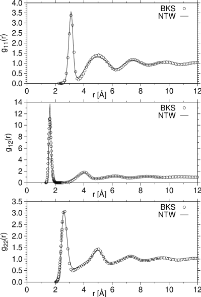
Figure 1: Partial pair correlation functions $g_{\alpha\beta}(r)$ for the NTW model (solid lines) and the BKS model for silica (open points). The thermodynamic state shown for BKS silica is $\rho=2.37\textrm{g}/\textrm{\AA}^{3},T=2750\textrm{K}$ and the one of NTW is $\rho=1.655,T=0.39$ in reduced units. The BKS data refer to the MD simulations by Horbach and Kob [30].

To reproduce the open, tetrahedral local structure of network glasses, two main physical ingredients must enter in the forcefield of our model: highly non-additive interaction radii and strong attraction between unlike species. Building on previous experience [26], we determined the following optimal set of interaction parameters:

$$\sigma_{12}/\sigma_{11}=0.49 \sigma_{22}/\sigma_{11}=0.85$$

$$\epsilon_{12}/\epsilon_{11}=6.00 \epsilon_{22}/\epsilon_{11}=1.00$$

To optimize the parameters above, we performed a series of preliminary simulations at reduced density $\rho=\rho_{expt}\approx 1.53$, which corresponds to the density of amorphous silica in normal experimental conditions. The parameters were adjusted by requiring that the ratio between the positions of the first peaks in $g_{12}(r)$ and $g_{11}(r)$ was equal to that of Si-O and Si-Si interatomic distances of amorphous silica. We also checked that at low temperature the average coordination numbers, obtained from the integral of the radial distribution functions, were close to the ideal tetrahedral ones, i.e., $Z_{12}=4$, $Z_{21}=2$.

Figure 2: Vibrational density of states (VDOS) obtained from local minima of the potential energy at $\rho=1.53$, $T=0.30$ for the NTW model (solid line), compared to experimental VDOS of amorphous silica (filled points, from [31]). The experimental data are convoluted with a correction function that alters their features only quantitatively [16].

The physical units of our model can be be fixed to reproduce some relevant properties of experimental and realistic models of silica, such as the BKS model. We fixed the length scale $\sigma_{11}$ so that the position of the first peak of $g_{11}(r)$ matched the mean Si-Si distance (i.e., $3.12\textrm{\AA}$) of amorphous silica. In this way we obtained $\sigma_{11}=2.84\textrm{\AA}$. To fix the energy scale $\epsilon_{11}$, we compared the shape of the radial distribution functions $g_{\alpha\beta}(r)$ to the ones obtained by Horbach and Kob [30] for BKS silica at the state point $\rho=2.37\textrm{g}/\textrm{\AA}^{3}$, $T=2750\textrm{K}$ (see figure 1). The corresponding density in reduced units is $\rho=1.655$. A good overall agreement of the liquid structure is found around $T=0.39$, from which we estimate $\epsilon_{11}\approx 7000\textrm{K}$. Finally, we fixed the time scale of our model by adjusting the mass scale $m_{1}$ so as to reproduce typical vibrational frequencies of amorphous silica. Following previous studies (see for instance [14, 15, 16]), we determined the vibrational density of states (VDOS) through diagonalization of the dynamical matrix calculated at local minima of the potential energy at $\rho=1.53$, $T=0.30$. The choice $m_{1}=8.7\times 10^{-23}\textrm{g}\approx 1.9m_{Si}$ yields reasonable agreement between the VDOS of our model and the experimental VDOS of amorphous silica [31] (see figure 2, which is further discussed in section 3). From the value of $m_{1}$ given above we obtain the time unit $t_{0}=\sqrt{m_{1}\sigma_{11}^{2}/\epsilon_{11}}=2.0\times 10^{-13}\textrm{s}$.

3 Structure and dynamics

In this section we further validate our model by analysing its structural and dynamical properties. Our simulations spanned a wide range of densities: $1.250\leq\rho\leq 2.300$. At higher density ($\rho=2.800$) we found clear signs of crystallization of our samples, but we did not attempt to determine the crystallographic structure. At lower densities ($\rho\leq 1.250$) large voids are formed in the network structure, and liquid-gas phase separation might occur. In the following, we will mostly focus on the isochore $\rho=1.655$, which corresponds to the density employed in several simulations of BKS silica, at temperatures in the range $0.29\leq T\leq 1.50$.

3.1 Structure and vibrations

The fact that the radial distribution functions of our model agree rather well with those of the more realistic BKS model (see figure 1) and the overall qualitative shape of the VDOS (see figure 2), already suggest that the NTW model should capture some relevant physical aspects of network glass-formers, at least for densities and temperatures where tetrahedral local ordering is more pronounced. In this section we study in more details the structural and vibrational properties of our model.

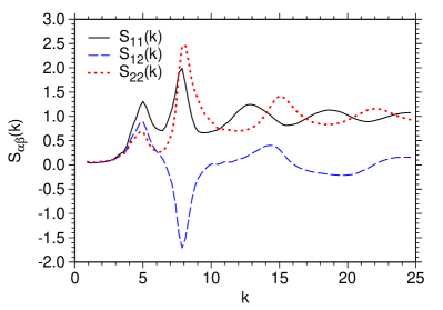
Figure 3: Partial structure factors $S_{11}(k)$ (solid line), $S_{12}(k)$ (dashed line), and $S_{22}(k)$ (dotted line) at $\rho=1.655$ and $T=0.29$.

In figure 3 we show the partial structure factors $S_{\alpha\beta}(k)$ obtained at the lowest temperature attained in equilibrium conditions for $\rho=1.655$. The pre-peak (also called first sharp diffraction peak) at $k\approx 5.0$ in $S_{11}(k)$ and $S_{22}(k)$ signals the formation of intermediate range order. This is a typical feature apparent at low temperature in network liquids. The positions of the pre-peak and main peak ($k\approx 8.0$) in $S_{11}(k)$ are in good agreement with those of $S_{SiSi}(k)$ in amorphous silica and simulated BKS silica [12].

Further insight into the structural properties of the NTW model is provided by the distribution $f_{\alpha\beta\gamma}(\theta)$ of angles formed by a central particle of species $\beta$ with neighbours of species $\alpha$ and $\gamma$, where $\alpha,\beta,\gamma=1,2$. Particles of species $\alpha$ and $\gamma$ are considered neighbours if their distance is less than the minimum of the radial distribution function at the corresponding $T$. The normalized angular distribution functions $f_{121}(\theta)$ and $f_{212}(\theta)$, shown in figure 4 for a few selected temperatures, reveal the typical features associated to local tetrahedral ordering. The broad peak in $f_{212}(\theta)$, located around $\theta=108^{\circ}$, reflects the presence of slightly distorted tetrahedra centered around particles of species 1. The $f_{121}(\theta)$ shows a peak around $180^{\circ}$, which corresponds the links formed by particles of species 2 connecting adjacent tetrahedra. Note that the peak positions and the overall shape of these distribution functions change only mildly below $T\approx 0.50$. Thus, below this temperature, which we will identify in the next section as the onset temperature of slow-dynamics [32], the NTW model displays a strong degree of tetrahedral local ordering.

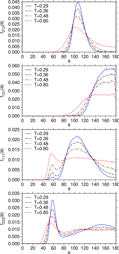
Figure 4: Angular distribution functions $f_{\alpha\beta\gamma}(\theta)$ for $T=0.80$ (dotted lines), 0.48 (dash-dotted lines), 0.36 (dashed lines), 0.29 (solid lines) at density $\rho=1.655$.

The angular distribution functions $f_{111}(\theta)$ and $f_{222}(\theta)$ (see two lower plots in figure 4) provide information about the intermediate range order of our model. The $f_{111}(\theta)$ displays a broad peak located at $\theta\approx 105^{\circ}$, associated to distorted corner-sharing tetrahedra. The smaller peak around $60^{\circ}$, due to three-fold rings [33], decreases in height upon lowering the temperature. At higher density ($\rho=2.300$, not shown here) this small peak increases in intensity (at fixed $T$), while the peak at $\theta\approx 105^{\circ}$ splits in two sub-peaks. Similar variations upon compression were found in the angular distribution functions of a more realistic model of silica [33]. Hence, we conclude that our simple model is able to capture some non-trivial structural features of network glass-formers.

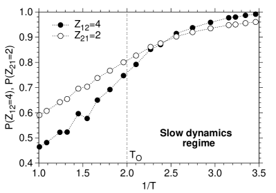
Figure 5: Fraction of particles with ideal tetrahedral coordination as a function of $1/T$: $P(Z_{12}=4)$ (empty circles) and $P(Z_{21}=2)$ (filled circles) are shown for particles of species 1 and 2, respectively. The vertical dotted line marks the onset of the slow-dynamics regime.

To highlight the formation of a nearly ideal tetrahedral network at low $T$, we show in figure 5 the $T$-dependence of the fraction of particles with ideal coordination numbers, i.e., $P(Z_{12}=4)$ and $P(Z_{21}=2)$ for particles of species 1 and 2, respectively. To identify neighbouring particles we used the same criterion as for the angular distribution functions discussed above. The fraction of ideally coordinated particles is already substantial around $T\approx 0.5$ [$P(Z_{12}=4),P(Z_{21}=2)>0.70$] and approaches unity at low $T$. This provides further indication that for the density considered here the system is indeed in the optimal region of network formation [25].

A closer inspection of figure 2 shows that the VDOS of the NTW model reproduces all the qualitative features of the experimental VDOS of amorphous silica. The relative positions of the peaks in the VDOS of NTW match well enough those of the experimental VDOS. Note that the absence of a peak at small frequencies ($\omega\approx 4$ THz) in the experimental data is due to insufficient experimental resolution [16, 34]. A careful comparison of simulated and experimental VDOS of silica can be found in [16]. Here we only recall that the VDOS of the BKS model is somewhat unrealistic at low and intermediate frequencies [16]. Similar deficiencies have also been found in recent modifications of the original BKS model employing short-ranged potentials [22]. Specifically, the distinct peaks at 12 and 24 THz, as well as the small peak around 18 THz ($D_{2}$ line), are missing in the VDOS of BKS silica. Given the simplicity of the forcefield employed, the success of the NTW model in reproducing the main qualitative vibrational features of amorphous silica is rather remarkable.

3.2 Relaxation dynamics

Our first step in the description of the dynamical properties of the NTW model consists in the identification of the so-called “slow-dynamics regime” [32]. In this temperature regime, the dynamical properties of glass-forming liquids assume all their distinct features, including two-step relaxation, dynamic heterogeneities, etc. To detect the onset of slow-dynamics, we study the variation with temperature of the incoherent intermediate scattering functions

$$F_{s}^{\alpha}(k,t)=\frac{1}{N_{\alpha}}\sum_{i=1}^{N_{\alpha}}\langle\exp\left\{i\boldsymbol{k}\cdot[\boldsymbol{r}_{i}(t)-\boldsymbol{r}_{i}(0)]\right\}\rangle$$ (3)

where $\alpha=1,2$ is an index of species. The $t$-dependence of $F_{s}^{1}(k,t)$ is shown in figure 6 for temperatures in the range $0.29\leq T\leq 1.50$ at two different wave-numbers: $k=5.0$, close to the pre-peak in the static structure factors (upper panel) and $k=8.0$ (lower panel). Two-step relaxation develops around $T_{O}\approx 0.50$, which we take as the onset temperature of the slow-dynamics regime. Distinct damped oscillations are observed in $F_{s}^{\alpha}(k,t)$ on the time scale of the early $\beta$-relaxation, i.e., on approaching the plateau. In larger samples (not shown here), the amplitude of these oscillations is slightly smaller—a well-known finite-size effect in model network liquids [30, 35].

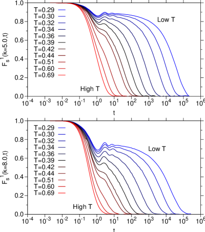
Figure 6: Intermediate scattering functions $F_{s}(k,t)$ (self part) at $\rho=1.655$ for wave-vector $k=5.0$ (top panel) and $k=8.0$ (bottom panel).

We now analyse the $T$-dependence of the structural relaxation times extracted from the intermediate scattering functions. Wave-number dependent relaxation times, $\tau_{\alpha}(k)$, for species $\alpha$ are defined by the condition $F_{s}^{\alpha}(k,\tau_{\alpha}(k))=1/e$. In the Angell plot in Fig. 7 we focus on the $T$-dependence of $\tau_{1}$. We focus here on the case $\tau\equiv\tau_{1}(k=5.0)$. To fit the $T$-dependence of the relaxation times we use the following modified Vogel-Fulcher equation, previously employed in our study of LJ mixtures [27],

$$\tau(T)=\left\{\begin{array}[]{ll}\tau_{\infty}\exp\left[E_{\infty}/T\right]&T>T^{*}\\ \tau_{\infty}^{{}^{\prime}}\exp\left[{\textstyle\frac{1}{K(T/T_{0}-1)}}\right]&T<T^{*}\\ \end{array}\right.$$ (4)

where

$$\tau_{\infty}^{{}^{\prime}}=\tau_{\infty}\exp\left[E_{\infty}/T^{*}-{\textstyle\frac{1}{K(T^{*}/T_{0}-1)}}\right]$$ (5)

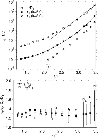
Figure 7: Top panel: Angell plot for structural relaxation times $\tau_{1}(k=5.0)$ (filled squares), $\tau_{1}(k=8.0)$ (stars), and inverse diffusion coefficients $1/D_{1}$ (empty squares). All quantities refer to particles of species 1. The modified VFT fit for $\tau_{1}(k=5.0)$ [equation (4)] and the Arrhenius fit for $1/D_{1}$ are also shown as solid lines. The dotted vertical line marks the onset of the slow dynamics regime. Lower panel: Ratios $\tau_{1}(k=5.0)/\tau_{2}(k=5.0)$ (filled squares) and $D_{2}/D_{1}$ (empty squares) as a function of $1/T$.

Equation (4) describes the crossover from Arrhenius to Vogel-Fulcher $T$-dependence of $\tau$, ensuring continuity at $T=T^{*}$. Its use in the case of a network glass-formers is justified by the observation that network liquids display a mild super-Arrhenius behaviour around and slightly below $T_{O}$. As we can see from figure 7, equation (4) fits rather well $\tau(T)$ over about 5 decades. Note that the degree of super-Arrhenius behaviour in $\tau(T)$ is indeed rather modest and more visible at wave-numbers corresponding to the first sharp diffraction peak ($k=5.0$).

Also included in figure 7 are the partial diffusion coefficients $D_{1}(T)$ obtained from the usual Einstein relation. To describe the $T$-dependence of the diffusion coefficients, we simply used the Arrhenius law, $D_{\alpha}=D_{\infty}^{\alpha}\exp(E_{\alpha}/T)$. By fitting the data at low temperature ($T<0.4$), we obtain activation energies $E_{1}=6.3\approx 3.8\textrm{eV}$ and $E_{2}=5.9\approx 3.6\textrm{eV}$, which are in reasonable agreement with those obtained in the case of BKS silica for silicon and oxygen atoms, respectively [30]. The difference in the diffusion coefficients between the two species is analysed in the lower panel of figure 7, where the ratio $D_{1}/D_{2}$ is shown as a function of $1/T$. This ratio becomes $\sim 2$ at the lowest temperatures. A smaller separation of time scales is found when inspecting the ratio $\tau_{2}/\tau_{1}$.

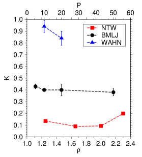
Figure 8: Fragility index $K$ obtained for NTW model and two representative LJ mixtures as a function of $\rho$ (NTW, lower axis) and $P$ (LJ, upper axis).

The fragility index $K$ of the NTW model obtained from fits to equation (4) is shown in figure 8 as a function of $\rho$. The system is slightly stronger (smaller $K$) at densities close to the experimental density of silica. In this range of density ($1.5<\rho<1.8$), tetrahedral local order becomes nearly ideal at low $T$. Hence, our results provide support for the link between structure and dynamic behaviour in network liquids demonstrated in [24] for patchy colloidal particles. Interestingly, the fragility of the NTW model seems to increase outside the density range mentioned above both at high and low density. Further investigations at low density would be required to clarify the nature of this behaviour and its possible connection with a reversibility window [36, 37], whose existence for silica has been suggested by recent work [38].

The use of a common functional form to describe $\tau=\tau(T)$ of NTW and LJ models allows a direct comparison of their Angell’s fragility. To this end, we also included in figure 8 the values of $K$ obtained in [27] for the mixture of Kob and Andersen (BMLJ [39]) and the mixture of Wahnström (WAHN [40]). Clearly, both LJ mixtures have larger fragility indexes. Furthermore, the fragility index of NTW, $K=0.09$, obtained at $\rho=1.655$ is lower by around a factor of 3 than the lowest values found for LJ mixtures ($K=0.24$ for AMLJ-0.60 [27]). The fact that the fragility index was obtained at constant density for the NTW and constant pressure for the LJ mixtures does not affect substantially our conclusions. Moreover, even when considering the variation of $K$ with $\rho$, the largest fragility index of the NTW model ($K=0.20$ at $\rho=2.300$) is comparable to the lowest ones found in LJ mixtures [27]. Thus, despite the presence of super-Arrhenius behaviour around the onset of slow dynamics, our network glass-former is stronger than all LJ mixtures studied in [27], a fact which fits naturally in the Angell classification scheme. Moreover, our analysis does not exclude the occurrence, at low temperatures, of a fragile-to-strong transition—a scenario which has recently found support on the basis of an energy landscape approach [20].

3.3 Dynamic heterogeneity

Figure 8 shows that NTW, BMLJ, and WAHN may be considered as models of strong, intermediate, and fragile glass-formers, respectively. This offers the opportunity to investigate the main trends of variations of the dynamics in liquids with different fragility. In this section, we focus on the degree of dynamic heterogeneity of the above mentioned models.

As a simple measure of the degree of heterogeneity of the dynamics we will use the non-Gaussian parameter

$$\alpha_{2}(t)=\frac{3\langle\,r^{4}(t)\,\rangle}{5{\langle\,r^{2}(t)\,\rangle}^{2}}-1$$ (6)

which measures the deviation of the distribution of particles’ displacements $r(t)$ from a Gaussian distribution. Upon cooling the liquid below $T_{O}$, in fact, the distribution of particles’ displacements deviates progressively from a Gaussian and the amplitude of $\alpha_{2}$ increases. Within the late $\beta$-relaxation time scale, the non-Gaussian parameter of typical glass-forming liquids displays a broad peak, whose the position $t^{*}$ and the height $\alpha^{*}$ increase by decreasing temperature. The trends of variation of the maximum of the non-Gaussian parameter $\alpha_{2}^{*}$ have been found to follow qualitatively the behaviour of more refined dynamic indicators [3], such as those obtained from four-point correlations functions [41, 42].

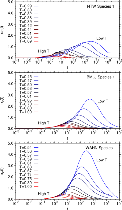
Figure 9: Non-Gaussian parameter $\alpha_{2}(t)$ for particles of species 1 along isochoric quenches for NTW at $\rho=1.655$ (top), BMLJ at $\rho=1.2$ (middle), and WAHN at $\rho=1.297$ (bottom).

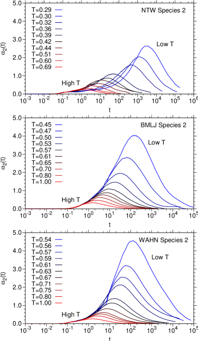
Figure 10: Same as Fig. 9 but for particles of species 2.

We computed the non-Gaussian parameter $\alpha_{2}(t)$ in equation (6) separately for species 1 and 2. The results obtained for NTW, BMLJ, WAHN models along isochoric quenches are shown in Fig. 9 and 10 for species 1 and 2, respectively. The degree of dynamic heterogeneity, as measured from the height $\alpha_{2}^{*}$ of the peak, is least pronounced in the case of the NTW model close to the ideal density for tetrahedral network structure. This is consistent with the analysis of Vogel et al [3], who found in fact that BKS silica had a lower degree of dynamic heterogeneity than other simple glass-formers, including the BMLJ model. Our results thus indicate a broad correlation between fragility and the degree of dynamic heterogeneity in glass-forming liquids. In particular, within the slow-dynamics regime, both the local structure and the local dynamics appear more homogeneous in network than in close-packed glass-formers.

3.4 Local rearrangements

We now turn to a closer inspection of the nature of local rearrangements in our model network glass-former. In particular, we want to identify the structural modifications that accompany relaxation events. This is motivated by the current interest in investigating the link between structure and dynamics in glass-forming liquids [43, 44]. We will contrast the results for the NTW model to those previously obtained for LJ systems [45, 27, 28].

In a first attempt to characterize the local dynamics of the NTW model and to establish a connection with its local structural properties, we computed the “propensity of motion” of particles, according to the definition of Widmer-Cooper et al [43]. In this approach, time-dependent atomic displacements $\Delta r(t)$, relative to a reference configuration, are averaged over several trajectories generated by independent initial sets of velocities (“iso-configurational ensemble”). The resulting spatial distribution of average displacements $\langle\Delta r(t)\rangle_{ic}$, where $\langle\dots\rangle_{ic}$ denotes an average in the iso-configurational ensemble, is thus strictly associated to the initial configuration, and can be used, in principle, to identify the local structural features responsible for relaxation events.

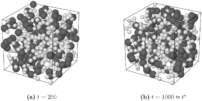
Figure 11: Snapshots of particles having large propensity of motion $\langle\Delta r(t)\rangle_{ic}$ for $t=200$ (left panel) and $t=1000\approx t^{*}$ (right panel). For both times, the 30% most mobile particles of either species are shown as large dark spheres, irrespectively of chemical species. The remaining particles are shown as small light spheres.

The spatial distribution of the particles with large propensity of motion for a representative configuration sampled at $T=0.31$ is shown in figure 11 for $t=200<t^{*}$ (left panel) and for $t=1000\approx t^{*}$ (right panel). Mobile particles, depicted in figure 11 as large dark spheres, are identified as the ones having the 30% largest propensities of motion among those of the same chemical species. The overall picture does not change upon small variation of the fraction of particles displayed. There is no substantial clustering of mobile particles on either time scales. Some clustering is observed at $t=1000$ but the size of the clusters remains rather modest (less than $\sim$ 10 neighbouring particles). This is strikingly different from the results obtained in LJ systems [45] within the slow-dynamics regime. In LJ systems, a pronounced clustering of particles with large propensity of motion has been observed for times on the order of the late $\beta$-relaxation ($t\approx t^{*}$). Our results confirm that the degree of dynamic heterogeneity of network liquids is much less pronounced than in close-packed LJ systems, and show that the origin of the weak dynamic heterogeneity observed within the $\alpha$-relaxation time scale is essentially kinetic, rather than structural.

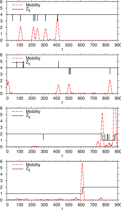
Figure 12: Instantaneous mobility $\mu_{i}(t)$ in arbitrary units (dashed line) for two representative particles of species 1 (two upper panels) and species 2 (two lower panels) at $T=0.29$. Also shown are the instantaneous coordination numbers $Z_{12}(t)$ and $Z_{21}(t)$ for particles of species 1 and 2, respectively (solid lines).

The results above do not imply, however, that there is no link at all between local structure and dynamics in network liquids. Such a link is more subtle and requires a different type of investigation. The breaking and reformation of bonds involved in typical relaxation events [30] occurs, in fact, on a very short time scale and the averaging introduced by the iso-configurational ensemble washes out this information. To overcome this problem we calculated, following Ladadwa and Teichler [46], the instantaneous mobility of particles from a smoothed atomic trajectory

$$\bar{\boldsymbol{r}}_{i}(t)=\int_{-\infty}^{\infty}\boldsymbol{r}_{i}(t^{\prime})\phi(t^{\prime},t)dt^{\prime}$$ (7)

where $\phi(t^{\prime},t)$ is a smoothing function normalized to 1. Rather than a Gaussian [46], we used a simple window smoothing function of length $2\Delta t$, which equals $1/(2\Delta t)$ for $t-\Delta t<t^{\prime}<t-\Delta t$ and 0 otherwise. From the smoothed trajectories, we computed the instantaneous atomic mobility [46]

$$\mu_{i}(t)^{2} = \int_{-\infty}^{\infty}[\bar{\boldsymbol{r}}_{i}(t)-\bar{\boldsymbol{r}}_{i}(t^{\prime})]^{2}\phi(t^{\prime},t)dt^{\prime}$$

$$= \frac{1}{2\Delta t}\int_{t-\Delta t}^{t+\Delta t}[\bar{\boldsymbol{r}}_{i}(t)-\bar{\boldsymbol{r}}_{i}(t^{\prime})]^{2}dt^{\prime}$$

using $\Delta t=10$. The time dependence of $\mu_{i}(t)$ is shown in figure 12 for representative particles of species 1 and 2 at $T=0.29$. At this low temperature, atomic mobilities show intermittent behaviour, with long periods of inactivity (vibrations) followed by displacements occurring on a very short time scale. To establish the connection with the changes in the local structure, we also plot, for the same time interval, the instantaneous coordination number $Z(t)$. A clear correlation between intermittent dynamical events and bond breaking and reformation processes is observed. In particular, defective local environments ($Z_{12}\neq 4$ and $Z_{21}\neq 2$), either created instantaneously by thermal fluctuations or associated to long-lived defective configurations, are closely associated to dynamical events. Interestingly, this shows that in network liquids the link between structure and dynamics can be understood at a single-particle level. Such a link has been demonstrated in LJ systems only at a coarse-grained spatial level [47].

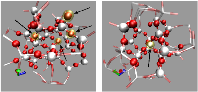
Figure 13: Animations of representative elementary dynamical events at $T=0.29$ (see http://www-dft.ts.infn.it/media/gp/1/ for the corresponding MPG files, realized with VMD [48]). White large spheres and small red spheres correspond to particles of species 1 and 2, respectively. The particles involved in the elementary dynamical events are surrounded by a yellow halo. Atomic positions have been averaged over a time window of 4.2 reduced time units (700 time steps) to remove thermal motion and help visualization. Left panel: four small particles (indicated by arrows in the figure) in the central-upper part of the figure perform a correlated, rotational motion in neighbouring tetrahedra (file movie1.mpg; size: 1.4 Mb). Right panel: the central particle (indicated by an arrow) explores its low density environment with a sequence of two jumps, associated to bond breaking and reformation (file: movie2.mpg; size: 1.7 Mb).

Finally, we describe qualitatively the typical local rearrangements observed at low temperature in the NTW model. By inspection of animated atomic trajectories, we identified two typical relaxation processes, closely related to the ones occurring in BKS silica. See figure 13 and supplementary materials (available at http://www-dft.ts.infn.it/media/gp/1/) for two representative events. A first class of rearrangements involves correlated rotations of tetrahedra formed by small particles around nearly immobile large particles. The overall process resembles the “rotational period” recently described by Heuer and coworkers [49], in which oxygens perform permutation of the tetrahedral positions around a fixed silicon atom. A second class of rearrangements is closely related to the ones described by Horbach and Kob [30]. One large particle jumps out from one of the faces of the tetrahedron surrounding it and attaches itself to an under-coordinated ($Z_{21}=1$) small particle. At the same time, a slight recoil movement of the small particles forming the involved tetrahedron is observed, together with the formation of a new dangling bond. Contrary to rotational rearrangements, which often involve a few neighbouring tetrahedra, this second class of elementary dynamical events is strongly localized around the involved tetrahedron. On longer time scales, however, sequences of independent events are also observed (see right panel of figure 13).

4 Stationary points and unstable modes

Summarising our previous analysis, two key features characterize the dynamical behaviour of our model network liquid: strong behaviour in the Angell’s classification scheme and a significant homogeneity of atomic displacements within the late $\beta$-relaxation time scale. In this section, we rationalize these features in terms of the properties of the Potential Energy Surface (PES). In particular, we first provide an estimate of the average energy barriers in the PES of the NTW model, and then analyse the localization properties and real-space structure of the unstable modes associated to stationary points of the PES.

4.1 Energy barriers

The nature and distribution of barriers connecting stationary points of the PES have been long recognized as key aspects for understanding the dynamics of fragile and strong liquids [6, 7]. Recently, sophisticated analysis of transitions between meta-basins for model glass-forming liquids [50] have provided even further quantitative evidence of the importance of the PES. In this section, we employ a simple definition of average energy barriers [51, 28] to quantify the roughness of the potential energy surface of the NTW model.

Our analysis of the PES is based on the procedure described in [28]. For each state point, we perform minimizations of the mean square total force $W$ to locate the closest stationary points along the dynamical trajectory. Typically, between 100 and 400 configurations per state point are considered as starting points for $W$-minimizations. It is well known that $W$-minimizations often locate points with a low value of $W$ ($W\approx 10^{-2}\div 10^{-4}$) that are not true stationary points. These points, usually called quasi-saddles, contain nonetheless relevant information about the dynamics [52, 53]. In the following, we will include these points in our analysis, without further distinction between true stationary points and quasi-saddles. Having located the stationary points, we diagonalize the Hessian matrix of the potential energy surface and thus obtain a set of $3N$ eigenfrequencies $\omega_{\alpha}$ and eigenvectors $\{\boldsymbol{e}_{i}^{\alpha}\}$. The unstable eigenvectors ($\omega_{\alpha}^{2}<0$) are of particular interest for our discussion, because they are more directly related to the dynamical behaviour of the system [45]. As in previous work [28], we will report the imaginary branch of the frequency spectrum along the real negative axis.

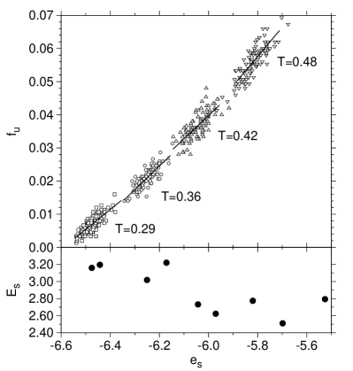
Figure 14: Upper plot: fraction of unstable modes $f_{u}$ as a function of the energy $e_{s}$ of individual stationary points sampled at the indicated temperatures. Also included are linear fits, from which the average energy barriers $E_{s}$ are obtained. Lower panel: average energy barriers $E_{s}$ as a function of the average energy of stationary points $e_{s}=e_{s}(T)$ for various $T$.

To estimate the average potential energy barriers we follow the definition given by Cavagna [51]

$$E_{s}=\frac{1}{3}\frac{de_{s}}{df_{u}}$$ (8)

where $e_{s}=e_{s}(f_{u})$ is the average energy of stationary points having a fraction of unstable modes $f_{u}=n_{u}/3N$. As in [28], we evaluate $E_{s}$ from the slope obtained by linear regression of $e_{s}$ vs. $f_{u}$ of individual stationary points sampled at temperature $T$. The procedure is illustrated in the upper panel of figure 14, where $f_{u}$ is shown as a function of $e_{s}$ for stationary points sampled at selected temperatures ($T<T_{O}$). The energy barriers obtained for individual state points are collected in the bottom panel as a function of the average energy of stationary points $e_{s}=e_{s}(T)$.

From the comparison of the results above with those obtained in [28] for LJ mixtures, we draw two main conclusions, which highlight the peculiarity of the network liquids: (i) energy barriers in the NTW model are large compared to typical thermal energies already for $T\approx T_{O}$, and (ii) their increase is very weak (less than 20%) with decreasing temperature below $T_{O}$. At least at a qualitative level, (ii) confirms our conjecture [28] that the fragility of a glass-forming liquid is related to the increase of average energy barriers $E_{s}$ upon cooling below $T_{O}$. It also supports the overall picture that the energy landscape of network liquids has a uniformly rough structure, with barriers whose average amplitude is nearly independent of the energy level. Organization of stationary points into meta-basin structures, while present even in network liquids [54], should be of much more limited extent than in the more fragile, close-packed glass-formers.

4.2 Localization properties

We now investigate the localization properties and the real-space structure of the unstable eigenvectors of the stationary points sampled in the slow-dynamics regime. In particular, we aim at explaining the more “homogeneous” character of atomic displacements observed in NTW, compared to the more fragile LJ mixtures.

Figure 15: Average gyration radius $L_{c}$ of modes of frequency $\omega$ calculated at $\rho=1.655$ and $T=0.31$ using different procedures (see text for definitions): straightforward calculation using equation (9) (dotted line), method (i) (dashed line), and method (ii) (solid line).

One possible measure of the degree of mode localization, used in a number of previous investigations [55, 56, 57], is provided by the gyration radius

$$L_{c}^{\alpha}=\sum_{i=1}^{N}{|e_{i}^{\alpha}|}^{2}|\boldsymbol{r}_{i}-\boldsymbol{r}_{c}|^{2}$$ (9)

where $r_{c}=\sum_{i=1}^{N}\boldsymbol{r}_{i}{|e_{i}^{\alpha}|}^{2}$ is the “centre of mass” of the mode. Extended modes should have $L_{c}\approx 1.0$, while $L_{c}<1.0$ for localized modes. It turns out, however, that the definition in equation (9) is inappropriate for systems with periodic boundary conditions. The centre of mass of the mode, in fact, is not well defined in a periodic system, and the value of $L_{c}$ thus depends on the choice of the origin of the frame of coordinates. As it will be clear in the following, this shortcoming is particularly evident in the case of strongly localized modes. To overcome this problem, we employ two alternative definitions of the gyration radius, obtained by redefining the origin of the system coordinates: (i) the position of the particle that has the largest displacement on mode $\alpha$ is used as the origin of the system coordinates for the calculation of $L_{c}^{\alpha}$; (ii) the gyration radius is determined by minimization of $L_{c}^{\alpha}$ over all possible origins of the system coordinates chosen on a grid of points subdividing the cubic cell.

Figure 16: Distribution of $L_{c}$ for unstable modes sampled in the slow-dynamics regime: in NTW at $\rho=1.655$, $T=0.31$ (upper panel), in BMLJ at $\rho=1.2$, $T=0.45$ (middle panel), in WAHN at $\rho=1.297$, $T=0.54$ (lower panel).

In figure 15 we show the average gyration radius $L_{c}$ of modes with frequency $\omega$ obtained for NTW at $T=0.31$, using the original definition and the two alternatives (i) and (ii). The original definition substantially overestimates the extension of strongly localized modes, while discrepancies are somehow less pronounced for extended modes. For extended modes, smaller discrepancies are apparent between methods (i) and (ii). In the following, we will employ definition (ii). Only minor quantitative differences in the following analysis appear when using definition (i).

We now focus on the unstable modes, which have been found to contain direct information on the dynamics of a glass-forming liquid [45]. In figure 16 we show the distribution of $L_{c}$ for the NTW model at $T=0.29$. For comparison, we also show analogous distributions obtained for BMLJ and WAHN at temperatures deep in the slow-dynamics regime. The distribution of $L_{c}$ for NTW is bimodal, with an excess of localized unstable modes having $L_{c}\sim 0.2$. A similar, yet much less pronounced, excess peak at low $L_{c}$ is observed in the distribution for BMLJ, while no such feature is found for the very fragile WAHN model. Justified by the fact that the minimum of the distribution of $L_{c}$ for NTW is located around 0.5, we define a mode localized (extended) if $L_{c}$ is smaller (larger) than 0.5. The precise location of this cutoff is irrelevant for the discussion below.

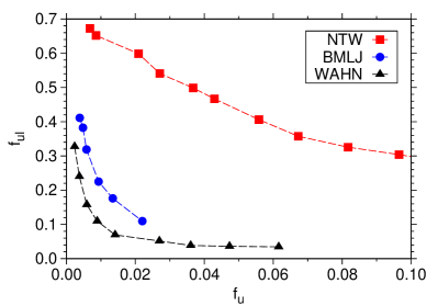
Figure 17: Fraction of localized unstable modes $f_{ul}$ in stationary points as a function of the total fraction unstable modes $f_{u}$ in NTW at $\rho=1.655$ (squares), BMLJ at $\rho=1.2$ (circles), and WAHN at $\rho=1.297$ (triangles).

Information about the relevance of localized unstable modes in different glass-formers is conveniently represented by the plot in figure 17, where the fraction of localized unstable modes $f_{ul}$ is shown as a function of $f_{u}$. The NTW model has a substantial fraction of localized unstable modes, independent of the energy level in the PES. $f_{ul}$ only weakly increases by lowering $f_{u}$, i.e., as the systems explores lower regions of the energy landscape. In contrast, in the very fragile WAHN $f_{ul}$ is very small and increases only on approaching the bottom of the energy landscape. The BMLJ displays an intermediate trend, since a larger fraction of localized unstable modes is present. These localized modes of the BMLJ mixture correspond to eigenvectors where a small particle and few other neighbours have large displacements (see figure 13 in [28]). It is remarkable that the trend observed in the localization of unstable modes follows the different dynamic character (strong, intermediate, fragile) of the models studied (see also [58]). Moreover, our results provide a simple explanation of the weak degree of dynamic heterogeneity in network liquids in terms of an excess of localized, uncooperative unstable modes, which are absent, or at least rarer, in the more fragile LJ mixtures.

Finally, we describe the nature of the rearrangements associated to localized and extended unstable modes of the NTW model. The typical extensions of localized and extended unstable modes are depicted in figure 18. From inspection of the real-space structure of the atomic displacements we found that the unstable modes reproduce the two classes of local relaxation processes described in section 3. Extended unstable modes usually involve coupled rotations of tetrahedra and have a marked collective nature. These modes are thus good candidates for explaining the rotational motions described in section 3. Similar unstable modes have been found in the unstable branch of the instantaneous normal mode spectrum of BKS silica [19]. On the other hand, localized unstable modes correspond rather well to the second class of local rearrangements described in section 3. The mode depicted in left panel of figure 18 shows the passage of a large particle, initially at the centre of a tetrahedron, through the face of the tetrahedron, while a neighbouring under-coordinated small particle moves in the opposite direction to create a bond. In the intermediate stage along the reaction coordinate of the mode the large particle is 5-fold coordinated. Our results indicate that both types of elementary dynamical events should be taken into account for a complete description of the dynamics in network liquids. Approaches that focus only on soft stable modes [59, 60] may not be able to capture the localized nature of the dynamics in network liquids. In these systems, in fact, the low frequency portion of the VDOS encompasses collective modes that typically involve coupled rotations of tetrahedra [61, 14].

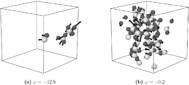
Figure 18: Typical extension of localized (a) and extended (b) unstable modes of a stationary point sampled at $T=0.29$. Only particles with displacement $|e_{i}^{\alpha}|$ larger than $0.04$ are shown, and the eigenvectors are scaled logarithmically. Particles of species 1 and 2 are shown as white large spheres and small dark spheres, respectively.

5 Conclusions

In this work we have extended our previous analysis [27, 28] on the glass transition of fragile Lennard-Jones mixtures by introducing a new model of tetrahedral network glass-former based on short-ranged, spherical interactions. Remarkably, these simple models of liquids, all based on pair potentials of the Lennard-Jones type, are able to reproduce qualitatively a wide spectrum of dynamic behaviours, thus allowing extensive and detailed investigations of the glass transition phenomenon.

Notwithstanding the problem of crystallization, which may occur in binary mixtures during longer simulations [62, 63] but is not observed in our samples, we have found that the fragile vs. strong behaviour of our models can be clearly identified and rationalized even at relatively high $T$, but below the onset temperature of slow dynamics. Using an appropriate parameterization of the $T$-dependence of relaxation times, we have found that the model network glass-former is stronger at all studied densities than all previously investigated LJ mixtures. Our results also confirm that the degree of dynamic heterogeneity is less pronounced in network than in close-packed glass-formers.

An important aspect of the glass transition concerns the nature of atomic rearrangements occurring within the $\alpha$-relaxation time [64, 65]. The relation between dynamical events and the nature of the local structure is of particular interest [43, 44]. The analysis of the propensity of motion of particles within the late $\beta$-relaxation time scale, combined with a comparative study of the non-Gaussian parameter in different systems, has revealed a substantial homogeneity of atomic mobility in the model network glass-former. However, contrary to the case of LJ mixtures, it is possible to establish a relation between local structure and dynamics at the single-particle level by considering individual atomic trajectories. Periods of high mobility are in fact clearly associated to sequences of bond breaking and reformation, i.e. variations in the local structure.

The features described above and the variation of dynamic behaviour in systems with different fragility can be rationalized well in terms of the features of the Potential Energy Surface. We have focused on the properties of the unstable modes of saddles and quasi-saddles sampled within the slow-dynamics regime. The amplitude of the average energy barriers $E_{s}$ in the model network glass-former is always larger than typical thermal energies below $T_{O}$ and depends very mildly on the energy level. This contrasts the findings in the more fragile LJ mixtures, where $E_{s}$ rapidly increases upon entering in the slow-dynamics regime [28]. The localization of the unstable modes offers direct insight into the elementary dynamic events leading to relaxation. In general, as the system explores lower and lower regions of the energy landscape, the unstable modes soften and retain a cooperative character. In the NTW model, there is also a significant fraction of localized unstable modes that persists in the whole slow-dynamics regime. These localized modes typically describe bond breaking and reformation, i.e. elementary rearrangements that characterize the dynamics of the model. On the contrary, close-packed fragile liquids have a large fraction of extended unstable modes, which soften and tend to localize only on approaching the bottom of the landscape. As a result, the dynamics in the latter systems is inherently more cooperative than in network liquids.

References

References

- [1] Angell C A 1988 J. Phys. Chem. Solids 49 863
- [2] Saika-Voivod I, Poole P H and Sciortino F 2001 Nature 412 514
- [3] Vogel M and Glotzer S 2004 Phys. Rev. E 70 061504
- [4] Berthier L 2007 Phys. Rev. E 76 011507
- [5] Garrahan J P and Chandler D 2003 Proc. Nat. Acad. Soc. 100 9710
- [6] Stillinger F H 1995 Science 267 1935
- [7] Debenedetti P G and Stillinger F H 2001 Nature 410 259
- [8] van Beest B W H, Kramer G J and van Santen R A 1990 Phys. Rev. Lett. 64 1955
- [9] Saika-Voivod I, Sciortino F and Poole P H 2000 Phys. Rev. E 63 011202
- [10] Saika-Voivod I, Sciortino F, Grande T and Poole P H 2004 Phys. Rev. E 70 061507
- [11] Vollmayr K, Kob W and Binder K 1996 Phys. Rev. B 54 15808
- [12] Horbach J and Kob W 1999 Phys. Rev. B 60 3169
- [13] Horbach J and Kob W 2001 Phys. Rev. E 64 041503
- [14] Taraskin S N and Elliott S R 1997 Phys. Rev. B 56 8605
- [15] Taraskin S N and Elliott S R 1999 Phys. Rev. B 59 8572
- [16] Benoit M and Kob W 2002 Europhys. Lett. 60 269
- [17] Jund P and Jullien R 1999 Phys. Rev. Lett. 83 2210
- [18] Nave E L, Stanley H E and Sciortino F 2002 Phys. Rev. Lett. 88 035501
- [19] Bembenek S D and Laird B B 2001 J. Chem. Phys. 114 2340
- [20] Saksaengwijit A, Reinisch J and Heuer A 2004 Phys. Rev. Lett. 93 235701
- [21] Kerrache A, Teboul V and Monteil A 2006 Chem. Phys. 321 69
- [22] Carré A, Berthier L, Horbach J, Ispas S and Kob W 2007 J. Chem. Phys. 127 114512
- [23] Ford M H, Auerbach S M and Monson P A 2004 J. Chem. Phys. 121 8415
- [24] De Michele C, Tartaglia P and Sciortino F 2006 J. Chem. Phys. 125 204710
- [25] Zaccarelli E, Sciortino F and Tartaglia P 2007 J. Chem. Phys. 127 174501
- [26] Ferrante A and Tosi M P 1989 J, Phys.: Condens. Matter 1 1679
- [27] Coslovich D and Pastore G 2007 J. Chem. Phys. 127 124504
- [28] Coslovich D and Pastore G 2007 J. Chem. Phys. 127 124505
- [29] Grigera T, Cavagna A, Giardina I and Parisi G 2002 Phys. Rev. Lett. 88 055502
- [30] Horbach J, Kob W, Binder K and Angell C A 1996 Phys. Rev. E 54 5897(R)
- [31] Carpenter J M and Price D L 1985 Phys. Rev. Lett. 54 441
- [32] Sastry S, Debenedetti P G and Stillinger F H 1998 Nature 393 554
- [33] Jin W, Kalia R K, Vashishta P and Rino J P 1994 Phys. Rev. B 50 118
- [34] Wischnewski A, Buchenau U, Dianoux A J, Kamitakahara W A and Zarestky J L 1998 Phys. Rev. B 57 2663
- [35] Guillot B and Guissani Y 1997 Phys. Rev. Lett. 78 2401
- [36] Phillips J C 1981 J. Non-Cryst. Solids 43 37
- [37] Thorpe M F 1983 J. Non-Cryst. Solids 57 355
- [38] Trachenko K and Dove M T 2003 Phys. Rev. B 67 212203
- [39] Kob W and Andersen H C 1995 Phys. Rev. E 51 4626
- [40] Wahnström G 1991 Phys. Rev. A 44 3752
- [41] Berthier L, Biroli G, Bouchaud J, Kob W, Miyazaki K and Reichman D R 2007 J. Chem. Phys. 126 184503
- [42] Berthier L, Biroli G, Bouchaud J, Kob W, Miyazaki K and Reichman D R 2007 J. Chem. Phys. 126 184504
- [43] Widmer-Cooper A, Harrowell P and Fynewever H 2004 Phys. Rev. Lett. 93 135701
- [44] Widmer-Cooper A and Harrowell P 2005 J. Phys.: Condens. Matter 17 S4025
- [45] Coslovich D and Pastore G 2006 Europhys. Lett. 75 784
- [46] Ladadwa I and Teichler H 2006 Phys. Rev. E 73 031501
- [47] Berthier L and Jack R L 2007 Phys. Rev. E 76 041509
- [48] Humphrey W, Dalke A and Schulten K 1996 J. Mol. Graphics 14 33
- [49] Saksaengwijit A and Heuer A 2007 J. Phys.: Condens. Matter 19 205143
- [50] Heuer A 2008 J. Phys.: Condens. Matter 20 373101
- [51] Cavagna A 2001 Europhys. Lett. 53 490
- [52] Angelani L, Di Leonardo R, Ruocco G, Scala A and Sciortino F 2002 J. Chem. Phys. 116 10297
- [53] Angelani L, Ruocco G, Sampoli M and Sciortino F 2003 J. Chem. Phys. 119 2120
- [54] Heuer A and Buchner S 2000 J. Phys,: Condens. Matter 12 6535
- [55] Marinov M and Zotov N 1997 Phys. Rev. B 55 2938
- [56] Caprion D and Schober R 2001 J. Chem. Phys. 114 3236
- [57] Ispas S, Zotov N, Wispelaere S D and Kob W 2005 J. Non-Cryst. Solids 351 1144
- [58] Jagla E A 2001 Mol. Phys. 99 753
- [59] Brito C and Wyart M 2007 J. Stat. Mech.: Theory Exp. 2007 L08003
- [60] Widmer-Cooper A, Perry H, Harrowell P and Reichman D R 2008 Nat. Phys. 4 711
- [61] Buchenau U, Zhou H M, Nucker N, Gilroy K S and Phillips W A 1988 Phys. Rev. Lett. 60 1318
- [62] Pedersen U R, Bailey N P, Dyre J C and Schrøder T B 2007 arXiv:0706.0813
- [63] Valdes L, Affouard F, Descamps M and Habasaki J 2009 J. Chem. Phys. 130 154505
- [64] Appignanesi G A, Rodriguez Fris J A, Montani R A and Kob W 2006 Phys. Rev. Lett. 96 057801
- [65] Appignanesi G A, Rodriguez Fris J A and Frechero M A 2006 Phys. Rev. Lett. 96 237803