Structured and unstructured continuous models for Wolbachia infections

Abstract

We introduce and investigate a series of models for an infection of a diplodiploid host species by the bacterial endosymbiont Wolbachia. The continuous models are characterized by partial vertical transmission, cytoplasmic incompatibility and fitness costs associated with the infection. A particular aspect of interest is competitions between mutually incompatible strains. We further introduce an age-structured model that takes into account different fertility and mortality rates at different stages of the life cycle of the individuals. With only a few parameters, the ordinary differential equation models exhibit already interesting dynamics and can be used to predict criteria under which a strain of bacteria is able to invade a population. Interestingly, but not surprisingly, the age-structured model shows significant differences concerning the existence and stability of equilibrium solutions compared to the unstructured model.

Keywords Wolbachia, cytoplasmic incompatibility, age-structured population dynamics, stability analysis

1 Introduction

Wolbachia is a maternally transmitted bacterium that lives in symbiosis with many arthropod species and some filarial nematodes [25, 16]. It inhabits testes and ovaries of its hosts and has the ability to interfere with their reproductive mechanisms, resulting in a variety of phenotypes. Well known effects are cytoplasmic incompatibility, induction of parthenogenesis, and feminization of genetic males, depending on the host species and the Wolbachia type. Besides the intrinsic interest in these mechanisms, Wolbachia are investigated as tools to drive desirable genes into a target population [17], as reinforcers of speciation [20, 21, 12], and as potential means of biological control [14]. It was recently shown by McMeniman et al. [14] that infection with Wolbachia shortens the life span of the mosquito Aedes aegypti, a vector for the Dengue fever virus. Since only older mosquitoes are carriers, this is a promising strategy to reduce the transmission of pathogens, without the ethically untenable eradication of a vector species.

Beginning already a half a century ago [1], various mathematical models for the spread of a Wolbachia infection have been proposed and studied in the literature, see e.g. [22, 17, 20, 12, 4, 18, 23, 9] and references therein. Largely, these models fall into two classes, depending on whether time proceeds in discrete steps or continuously. Examples for continuous models are the papers [12] and [18] that employ ordinary, respectively partial differential equations (with a spatial structure in the latter case). In their paper [12], the authors proposed and studied a simple continuous model for the infection of an arthropod population with cytoplasmic incompatibility (CI) causing Wolbachia. Cytoplasmic incompatibility in diplodiploid (i.e. with diploid males and females) species manifests itself in completely or partially unviable crosses of infected males with uninfected females. For a discussion of the more complex outcome of cytoplasmic incompatibility in haplodiploid species see [23].

In this paper, we introduce a series of models for different aspects of interest. We start in section 2 with an ordinary differential equation model for a single Wolbachia strain that infects a population without separate sexes. In section 3 we present a model for infections with multiple strains. The present theoretical literature offers a complex picture of infection with multiple strains. While some authors exclude the coexistence of multiple strains of Wolbachia in infected individuals [12, 9], others model doubly infected individuals as a class of their own [4, 23]. Moreover, different assumptions are made about the mutual compatibility of individuals carrying different strains. We construct a general model that encompasses these different possibilities by suitable choices of parameter values and/or initial conditions. Finally, motivated by the study [14], in section 4 we refine our model from section 2, by considering age-structured populations. We refer the interested reader for basic concepts and results in structured population dynamics to [2, 15, 24]. Modeling structured populations usually involves partial differential equations which are more difficult to analyze. Analytical progress is still possible, and as we will see in 4, the age-structured model may exhibit richer dynamics. At this point it will be possible to study age-dependent killing of Wolbachia infected individuals. Our models contain parameters of only three types, namely transmission efficacies, levels of cytoplasmic incompatibility and fitness costs for the infected individuals. The analysis of the models aims to give conditions for the stability of specific equilibrium solutions that correspond to successful invasions. The paper ends with a discussion in section 5 and an outlook on future work.

2 Single-sex model for a singular Wolbachia strain

Assume that the ratio of infected males to infected females is the same as the ratio of uninfected males to uninfected females and hence the population can be formally considered hermaphroditic. Let $I$ and $U$ denote the number of infected, respectively uninfected individuals in the population. Vertical transmission is partial, let $\tau\in[0,1]$ be the fraction of infected offspring from infected parents (another common notation is $\mu=1-\tau$ for the fraction of uninfected ova produced by an infected female, see e.g. [22, 16, 23]). Furthermore, we follow Keeling et al. [12] and assume that the birth rate for both infected and uninfected individuals is equal (no reduction in fecundity in infected individuals). Let this rate be denoted by $b>0$. Death of the individuals is modelled by a logistic loss term with rate $d>0$ that accounts for competition among the total population. However, infected individuals can suffer an additional loss of fitness given by $D\geq 0$. Cytoplasmic incompatibility arises when an infected male fertilizes an egg from an uninfected female. Then, with a probability $q\in[0,1]$, the offspring is nonviable. As we do not consider separate sexes in this simple model, we just reduce the amount of offspring from uninfected individuals based on the probability of an encounter with an infected individual. Uninfected individuals still arise due to incomplete transmission of the bacterium from infected parents. Our equations read

$$\frac{dI}{dt} =\left(\tau b-(d+D)(I+U)\right)I,$$

$$\frac{dU}{dt} =(1-\tau)bI+\left(b\left(1-q\frac{I}{I+U}\right)-d(I+U)\right)U.$$

Upon rescaling the time by $t\rightarrow bt$ and setting $\eta=\frac{d+D}{d}$, we obtain the reduced system for the quantities $i=dI/b$, $u=dU/b$

$$\frac{di}{dt} =(\tau-\eta(i+u))i,$$ (1)

$$\frac{du}{dt} =(1-\tau)i+\left(1-q\frac{i}{i+u}-(i+u)\right)u.$$ (2)

Observe that $\eta^{-1}=:\xi\in(0,1]$ and that $1-\xi$ can be interpreted as the fitness cost associated with Wolbachia infection. The point $(0,0)$ can be added to the domain of the state space, with the understanding that it is an equilibrium solution. It is obvious that the subspace of uninfected populations $\{0\}\times\mathbb{R}$ is forward invariant (that is, if initially there are no infected individuals, then there will be none at later times) and if transmission is complete, $\tau=1$, then so is the subspace of completely infected populations $\mathbb{R}\times\{0\}$.

Equation (1)–(2) always admits the disease free equilibrium

$$(i_{0},u_{0})=(0,1).$$ (3)

Setting the left-hand side of equation (1) to zero and solving for an equilibrium point $u$ yields

$$u=\tau\xi-i.$$ (4)

Inserting this into the equilibrium condition for (2) gives a quadratic equation for $i$,

$$\frac{q}{\tau\xi}i^{2}+(\tau(\xi-1)-q)i+\tau\xi(1-\xi\tau)=0.$$ (5)

Provided that

$$(\tau(\xi-1)-q)^{2}-4q(1-\xi\tau)\geq 0,$$ (6)

equation (5) has the solutions

$$i_{1}=i_{1}(q,\tau,\xi) =\frac{\tau\xi\left(q-\tau(\xi-1)-\sqrt{(\tau(\xi-1)-q)^{2}-4q(1-\xi\tau)}\right)}{2q},$$ (7)

$$i_{2}=i_{2}(q,\tau,\xi) =\frac{\tau\xi\left(q-\tau(\xi-1)+\sqrt{(\tau(\xi-1)-q)^{2}-4q(1-\xi\tau)}\right)}{2q},$$

these are always non-negative. The corresponding equilibrium values for the uninfected individuals are given by (4). For $u_{2}\geq 0$ it is necessary that

$$q+\tau(\xi-1)\geq 0.$$ (8)

This condition is also sufficient, since then one can derive from $\tau\leq 1$ the inequality

$$q+\tau(\xi-1)\geq\sqrt{(\tau(\xi-1)-q)^{2}-4q(1-\xi\tau)}$$

and hence $u_{2}\geq 0$. Condition (6) separates two regions in the parameter space, depending on whether other equilibrium solutions than the disease free equilibrium are possible (see figure 1). We calculate the Jacobian of the right hand side $F$ of (1)–(2),

$$DF(i,u)=\begin{pmatrix}\tau-\eta(2i+u)&-\eta i\!\\ \!1-\tau+qu\left(\frac{i}{(i+u)^{2}}-\frac{1}{i+u}\right)-u&1+qi\left(\frac{u}{(i+u)^{2}}-\frac{1}{i+u}\right)\!-(2u+i)\end{pmatrix}\!.$$ (9)

At the disease free equilibrium (3), we have

$$DF(0,1)=\begin{pmatrix}\tau-\eta&0\\ -\tau-q&-1\end{pmatrix},$$

this matrix has the eigenvalues $-1$ and $\tau-\eta\leq 0$. The latter eigenvalue is $0$ only if $\tau=1$ (complete transmission) and $D=0$ (no penalty for infection), in all other cases it is strictly negative, and the disease free equilibrium is locally asymptotically stable.

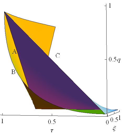
Figure 1: The yellow surface separates the $(\xi,\tau,q)$-parameter space of model (1)–(2) into a region where only the disease free equilibrium (3) exists (A) and where coexistence equilibrium solutions $(u_{1},i_{1})$ and $(u_{2},i_{2})$ given by (7) are possible (B). However, only in the region (C) above the blue surface given by (8) is $u_{2}=\tau\xi-i_{2}\geq 0$ (this belongs to the observed stable equilibrium $(u_{2},i_{2})$).

Explicit expressions (with respect to the parameters $q,\,\tau$ and $\xi$) can be obtained for the eigenvalues of the Jacobian (9) at the equilibrium solutions using e.g. mathematica (the mathematica notebook is available from the authors upon request). Unfortunately these expressions are very complicated and not easily analyzed. We will present instead some representative numerical examples to demonstrate the possible behaviours.

Example 2.1.

Assume that the infection is completely inherited, $\tau=1$, cytoplasmic incompatibility is complete $q=1$, and that the cost of the infection is low, $\xi=0.9$. Then the three equilibrium solutions $(i_{0},u_{0})=(0,1)$, $(i_{1},u_{1})=(0.09,0.81)$ and $(i_{2},u_{2})=(0.9,0)$ are present, of which $(i_{0},u_{0})$ and $(i_{2},u_{2})$ are locally asymptotically stable. The vector field is shown in figure 2 (left panel). The epidemic equilibrium $(i_{2},u_{2})$ has a much bigger basin of attraction than the disease free equilibrium $(i_{0},u_{0})$, in other words, the threshold for an infection to establish itself is low.

Example 2.2.

At high levels of cytoplasmic incompatibility, $q=1$, and no penalty for the infection, $\xi=1$, and a partial transmission $\tau=0.76$, besides the equilibrium $(i_{0},u_{0})$ there is the locally asymptotically stable coexistence equilibrium $(i_{2},u_{2})=(0.456,0.304)$, see figure 2 (right panel). The basin of attraction of the disease free equilibrium $(i_{0},u_{0})$ is much bigger than in example 2.1, indicating that the threshold for establishment of the infection is higher.

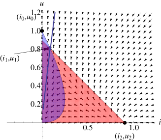
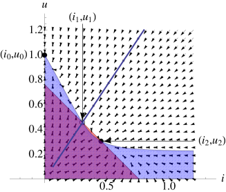
Figure 2: (Left) The vector field (1)–(2) for the parameter triple $(\xi,\tau,q)=(0.9,1,1)$ together with the three equilibrium solutions. Solid disks indicate locally asymptotically stable equilibrium solutions, while the disk indicates an unstable equilibrium. Shown are also regions of growth of $u$ (light blue) and growth of $i$ (light red). The blue lines are the stable manifolds of the saddle point $(i_{1},u_{1})$ and the separatrices of the equilibrium solutions $(i_{0},u_{0})$ and $(i_{2},u_{2})$. (Right) The vector field (1)–(2) for the parameter triple $(\xi,\tau,q)=(1,0.76,1)$, which admits bistability and true coexistence. The stable manifold of the saddle point $(i_{1},u_{1})$ is shown in blue.

Example 2.3.

If the cytoplasmic incompatibility is very weak, $q=0.1$ and the fitness cost of the infection is higher, $\xi=0.5$ (and again $\tau=1$), then the equilibrium $(i_{0},u_{0})=(0,1)$ is globally asymptotically stable in the set $\{i\geq 0,u\geq 0\}$ and the equilibrium $(i_{1},u_{1})=(0.5,0)$ is a saddle point. The third equilibrium point has $u_{2}<0$ and has no biological meaning.

The above examples suggest that the equilibrium $(i_{1},u_{1})$ is always a saddle and that $(i_{2},u_{2})$ is locally asymptotically stable, if $u_{2}\geq 0$. If $(i_{2},u_{2})$ exists and is locally asymptotically stable, then its basin of attraction is larger for larger values of the transmission rate $\tau$ (this is the intersection of regions (B) and (C) in figure 1).

3 Infection with multiple strains

Assume that two Wolbachia strains A and B are present in the population and let $i_{A},\,i_{B}$ and $i_{AB}$ denote the number of individuals singly or doubly infected, in addition to $u$, the number of uninfected individuals. We use the same scaling as in the previous section, where time was scaled with respect to the birth rate $b$. There are seven incompatibility levels $q_{X,Y}$ where $X,Y\in\{0,A,B,AB\}$ are the infection statuses in the incompatible cross. These are shown in the directed graph of incompatibilities in figure 3.

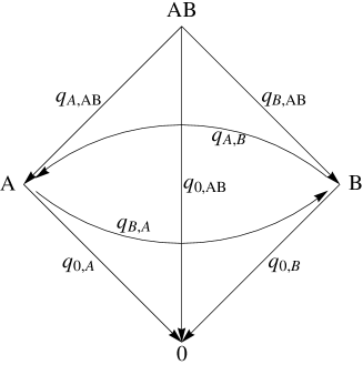
Figure 3: The directed graph of possible incompatibility relations. An arrow from node $X$ to node $Y$ indicates that a $X\male\times Y\female$ cross is incompatible, with incompatibility level $q_{Y,X}$.

We assume that the transmission of one strain in doubly infected individuals is independent of the transmission of the other strain [23]. Moreover, the mortalities due to infection with either strain are additive. With these assumptions, and setting $p=i_{AB}+i_{A}+i_{B}+u$ for the total population, our model is

$$\frac{di_{AB}}{dt} =\tau_{A}\tau_{B}i_{AB}-\eta_{AB}pi_{AB},$$ (10)

$$\frac{di_{A}}{dt} =\tau_{A}(1-\tau_{B})i_{AB}+\tau_{A}\left(1-q_{A,B}\frac{i_{B}}{p}-q_{A,AB}\frac{i_{AB}}{p}\right)i_{A}-\eta_{A}pi_{A},$$

$$\frac{di_{B}}{dt} =(1-\tau_{A})\tau_{B}i_{AB}+\tau_{B}\left(1-q_{B,A}\frac{i_{A}}{p}-q_{B,AB}\frac{i_{AB}}{p}\right)i_{B}-\eta_{B}pi_{B},$$

$$\frac{du}{dt} =(1-\tau_{A})(1-\tau_{B})i_{AB}+(1-\tau_{A})\left(1-q_{A,B}\frac{i_{B}}{p}-q_{A,AB}\frac{i_{AB}}{p}\right)i_{A}$$

$$\quad+(1-\tau_{B})\left(1-q_{B,A}\frac{i_{A}}{p}-q_{B,AB}\frac{i_{AB}}{p}\right)i_{B}$$

$$\quad+\left(1-q_{0,A}\frac{i_{A}}{p}-q_{0,B}\frac{i_{B}}{p}-q_{0,AB}\frac{i_{AB}}{p}\right)u-pu,$$

where

$$\eta_{A}=\frac{d+D_{A}}{d},\quad\eta_{B}=\frac{d+D_{B}}{d}\quad\textrm{and}\quad\eta_{AB}=\frac{d+D_{A}+D_{B}}{d}=\eta_{A}+\eta_{B}-1$$

are measures of the fitness costs of the individual infection types. This model can now be reduced in its complexity in a variety of ways. For example, if the initial condition lies in the space $\{0\}\times\mathbb{R}^{3}$, that is, there are no doubly infected individuals present initially, then the solution will also lie in that space at all times. Moreover, setting appropriate incompatibility levels $q_{X,Y}$ to zero allows to study cases of mutual compatibility.

As a first illustration, we want to consider the absence of doubly infected individuals, $i_{AB}\equiv 0$, mutual compatibility of infected individuals, $q_{A,B}=q_{B,A}=0$, equal transmission efficacy $\tau_{A}=\tau_{B}=:\tau$ and equal infection costs $\eta_{A}=\eta_{B}=:\eta$ (again, we write $\xi=\eta^{-1}$). The symmetry is only broken by the levels of incompatibility $q_{0,A}\neq q_{0,B}$. Hence, equation (10) simplifies to

$$\frac{di_{A}}{dt} =(\tau-\eta p)i_{A},$$ (11)

$$\frac{di_{B}}{dt} =(\tau-\eta p)i_{B},$$

$$\frac{du}{dt} =(1-\tau)(i_{A}+i_{B})+\left(1-q_{0,A}\frac{i_{A}}{p}-q_{0,B}\frac{i_{B}}{p}\right)u-pu.$$

Observe that model (11) has the property that planes orthogonal to the $(i_{A},i_{B})$-plane

$$R_{\alpha}=\left\{(i_{A},i_{B},u)\in\mathbb{R}_{\geq 0}^{3}\>:\>i_{A}-\alpha i_{B}=0\right\}$$

are invariant under the flow generated by (11). This is seen from the fact that for every $\alpha\in[0,\infty]$

$$\frac{d}{dt}(i_{A}-\alpha i_{B})=(\tau-\eta p)(i_{A}-\alpha i_{B})=0$$

on $R_{\alpha}$. This implies that the ratio $\frac{i_{A}}{i_{A}+i_{B}}$ remains constant along a trajectory. In other words, if transmission efficacies and death rates are equal for two strains (as are birth rates throughout in our model) then neither strain can replace the other among the infected individuals based on stronger cytoplasmic incompatibility. This is in line with recent theoretical predictions of Turelli [22] and Haygood and Turelli [9], who suggest that strains are selected for relative fecundity rather than high levels of cytoplasmic incompatibility. It needs to be pointed out however, that even a small difference in transmission efficacies or death rates of the two strains helps the strain with the greater transmission rate or the lower mortality to establish itself in the population.

The disease free equilibrium of (11) is easily found to be

$$(i_{A,0},i_{B,0},u_{0})=(0,0,1).$$ (12)

It is clear that the subspaces $\{0\}\times\mathbb{R}\times\mathbb{R}$ and $\mathbb{R}\times\{0\}\times\mathbb{R}$ are forward invariant under the flow generated by (11) and that the equilibrium solutions (7) exist in the respective subspaces, with $q$ in (7) replaced by either $q_{0,A}$ or $q_{0,B}$. That is, we have equilibrium solutions

$$(i_{A,1}(q_{0,A},\tau,\xi),0,\tau\xi-i_{A,1}), \quad(i_{A,2}(q_{0,A},\tau,\xi),0,\tau\xi-i_{A,2}),$$

$$(0,i_{B,1}(q_{0,B},\tau,\xi),\tau\xi-i_{B,1}), \quad(i_{B,2}(0,q_{0,B},\tau,\xi),\tau\xi-i_{B,2}).$$

Besides that, it can be checked that there is a continuum of equilibrium solutions

$$\begin{pmatrix}i_{A}(u)\\ i_{B}(u)\end{pmatrix}=\begin{pmatrix}\frac{-\tau^{3}-\eta q_{0,B}\tau u+\eta^{2}q_{0,B}u^{2}+\tau^{2}(1+(\eta-1)u)}{\eta^{2}(q_{0,A}-q_{0,B})u}\\ \frac{\tau^{3}+\eta q_{0,A}\tau u-\eta^{2}q_{0,A}u^{2}-\tau^{2}(1+(\eta-1)u)}{\eta^{2}(q_{0,A}-q_{0,B})u}\end{pmatrix}$$ (13)

for every $u\in(0,\tau\xi)$, provided that these expressions are non-negative. The solutions from (13) satisfy

$$i_{A}(u)+i_{B}(u)=\frac{\tau}{\eta}-u=\tau\xi-u,$$

which corresponds to equation (4).

Example 3.1.

We consider the case $\tau=1$ of complete transmission. One checks by direct calculation that system (11) then has another manifold of equilibrium solutions

$$i_{A}+i_{B}=\xi,\quad u=0.$$

The intersection of this line with each plane $R_{\alpha}$ orthogonal to the $(i_{A},i_{B})$-plane is an equilibrium for the flow restricted to that plane. In addition, each $R_{\alpha}$ contains a saddle point. A numerical example is shown in figure 4 (left panel). If, in contrast, different costs are associated with the infection, the strain with the lower cost will dominate the population, see figure 4 (right panel). Similarly, if infection costs are equal, but one strain transmits more efficiently, then it is going to dominate the population.

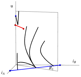
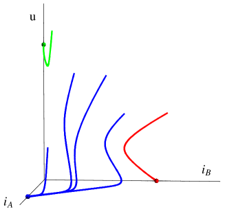
Figure 4: (Left) Dynamics of model (11) in the case that $q_{0,A}=0.95,\,q_{0,B}=0.5,\,\tau=1$ and $\eta=1.1$. The solid blue line is a family of attractors for the flow restricted to planes $R_{\alpha}$, the red line is a branch of saddle points in each of these subspaces. Several individual trajectories are shown, and the space $R_{1}=\{i_{A}=i_{B}\}$ is marked. (Right) If we choose instead $\eta_{A}=1.1$ and $\eta_{B}=1.2$ (while keeping all other parameters the same) then the less costly strain A dominates the population.

We return to model (10) and consider mutual incompatibility of singly infected individuals. The equations are

$$\frac{di_{A}}{dt} =\left(\tau\left(1-q_{A,B}\frac{i_{B}}{p}\right)-\eta p\right)i_{A},$$ (14)

$$\frac{di_{B}}{dt} =\left(\tau\left(1-q_{B,A}\frac{i_{A}}{p}\right)-\eta p\right)i_{B},$$

$$\frac{du}{dt} =\phantom{+}(1-\tau)\left(\left(1-q_{A,B}\frac{i_{B}}{p}\right)i_{A}+\left(1-q_{B,A}\frac{i_{A}}{p}\right)i_{B}\right)$$

$$\quad+\left(1-q_{0}\frac{i_{A}+i_{B}}{p}\right)u-pu.$$

It is clear that if either strain is not present initially then it will remain absent at all times. On the marginal spaces $\{i_{A}=0\}$ and $\{i_{B}=0\}$, equations (14) reduce to the single strain model (1)–(2) and have the corresponding equilibrium solutions where only one strain is present, with the common disease free equilibrium (12). It follows from (14) that

$$\frac{d}{dt}(q_{B,A}i_{A}-q_{A,B}i_{B}) =\phantom{-}q_{B,A}\left(\tau\left(1-q_{A,B}\frac{i_{B}}{p}\right)-\eta p\right)i_{A}$$

$$\quad-q_{A,B}\left(\tau\left(1-q_{B,A}\frac{i_{A}}{p}\right)-\eta p\right)i_{B}$$

$$=\phantom{+}\tau\left(q_{B,A}\left(1-q_{A,B}\frac{i_{B}}{p}\right)i_{A}-q_{A,B}\left(1-q_{B,A}\frac{i_{A}}{p}\right)i_{B}\right)$$

$$\quad-\eta p(q_{B,A}i_{A}-q_{A,B}i_{B})$$

$$=\left(\tau-\eta p\right)(q_{B,A}i_{A}-q_{A,B}i_{B}).$$

This implies that the plane orthogonal to the $(i_{A},i_{B})$-plane,

$$R_{*}=\left\{(i_{A},i_{B},u)\in\mathbb{R}_{\geq 0}^{3}\>:\>q_{B,A}i_{A}=q_{A,B}i_{B}\right\},$$

is forward invariant, and hence so are the wedges on either side. Solving equations (14) for the total population yields that if $i_{A}\neq 0$, $i_{B}\neq 0$

$$0 =p^{2}-\frac{\tau}{\eta}p+\frac{\tau}{\eta}q_{A,B}i_{B},$$

$$0 =p^{2}-\frac{\tau}{\eta}p+\frac{\tau}{\eta}q_{B,A}i_{A}.$$

For this system to be consistent, it is necessary that if $i_{A}\neq 0$, $i_{B}\neq 0$ then

$$q_{B,A}i_{A}=q_{A,B}i_{B},$$

hence any coexistence equilibrium of the two infected strains has to lie in the plane $R_{*}$. Indeed, there may be a saddle point equilibrium solution in $R_{*}$ that is locally asymptotically stable for flows that start in $R_{*}$.

Example 3.2.

Let $q_{A,B}=0.99$, $q_{B,A}$ and $q_{0,A}=q_{0,B}=1$. Choose the transmission efficacy $\tau=1$ and the cost of the infection $\eta=1.1$. We see in figure 5 that every solution starting outside the space $R_{*}$ converges to an equilibrium in one of the marginal spaces. The plane $R_{*}$ contains a locally stable equilibrium for trajectories starting in $R_{*}$ which has $u_{2}=0$ and it contains a saddle point for trajectories starting within $R_{*}$ (not shown, compare to example 2.1 and figure 2).

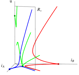
Figure 5: Mutually incompatible strains as described in (14) do not show coexistence. The marginal equilibrium solutions are marked by dots, the disease free equilibrium (equation (12), green) attracts some solutions from the plane $R_{*}$ and other trajectories beginning in the wedges on either side that are not shown here.

Again, we need to recall that this dynamical behaviour is not generic, in the sense that the complement of the set $\{\tau_{A}=\tau_{B},\,\eta_{A}=\eta_{B}\}$ is dense in the parameter space.

Finally, we want to explore the full model (10) when doubly infected individuals are present. To reduce the number of parameters somewhat, we assume

$$q_{A,B}=q_{A,AB}=q_{0,B},\quad q_{B,A}=q_{B,AB}=q_{0,A},$$

that is, the presence of one strain in the fertilizing male that is missing in the female has the same effect, regardless of the other infections that the female may carry [10, p.66]. Moreover, the escape from cytoplasmic incompatibility for the offspring of an uninfected female and a doubly infected male is the product of the two individual escape probabilities [23],

$$1-q_{0,AB}=(1-q_{0,A})(1-q_{0,B}).$$

Example 3.3.

Under the above assumptions, let $q_{A,B}=0.9=q_{B,A}$, the transmission efficacy $\tau_{A}=\tau_{B}=0.9$ and the cost of the infection $\eta_{A}=\eta_{B}=1.1$. Then there exists a coexistence equilibrium of doubly infected and both types of singly infected individuals, where however the proportion of doubly infected individuals is much larger (figure 6).

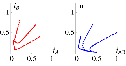
Figure 6: With the parameters chosen as described in example 3.3, we observe stable coexistence of all three infection types. Solid, dashed and dotted lines, respectively, show parts of the solution starting at the same initial values.

4 Introduction of age-structure

In the previous sections we have seen that infection with Wolbachia gives rise to interesting dynamic behaviour already in unstructured populations. Clearly, individuals of different ages are subject to different fertility and mortality rates. We therefore expand our model (1)–(2) to include age-dependent fertility and mortality rates for infected and uninfected individuals. This leads to nonlinear partial differential equations with nonlocal boundary conditions that represent the birth process [24, 5, 6, 8, 7]. Although this results in more complex models, they are still amenable to analytical study. Here we focus on qualitative questions, when analytical progress is possible; in particular, how do the stability results for equilibrium solutions compare to the unstructured case.

Let $i(a,t)$ and $u(a,t)$ denote the densities of infected and uninfected individuals of age $a$ at time $t$, respectively, where $a\in[0,m]$ (this is not to be confused with the notation in section 2, where they denoted scaled numbers of infected and uninfected individuals). Then the evolution of the population is governed by

$$i_{t}(a,t)+i_{a}(a,t) =-\eta_{1}(a)(I(t)+U(t))i(a,t),$$ (15)

$$u_{t}(a,t)+u_{a}(a,t) =-\eta_{2}(a)(I(t)+U(t))u(a,t),$$ (16)

$$i(0,t) =\tau\int_{0}^{m}\beta_{1}(a)i(a,t)\,\mathrm{d}a,$$ (17)

$$u(0,t) =(1-\tau)\int_{0}^{m}\beta_{1}(a)i(a,t)\,\mathrm{d}a$$

$$\quad+\left(1-q\frac{I(t)}{I(t)+U(t)}\right)\int_{0}^{m}\beta_{2}(a)u(a,t)\,\mathrm{d}a,$$ (18)

where

$$I(t)=\int_{0}^{m}\ i(a,t)\,\mathrm{d}a,\quad U(t)=\int_{0}^{m}\ u(a,t)\,\mathrm{d}a,$$

and $\eta_{1},\,\eta_{2},\,\beta_{1}$ and $\beta_{2}$ denote the age-specific mortality and fertility rates for infected and uninfected individuals, respectively. System (15)–(18) is equipped with initial conditions

$$i(a,0)=i_{0}(a),\quad u(a,0)=u_{0}(a).$$

The parameters $\tau$ and $q$ have the same meaning as in section 2.

4.1 Existence of equilibrium solutions

We find the time-independent solutions of equations (15) and (16) as

$$i_{*}(a) =i_{*}(0)\exp\left\{-(I_{*}+U_{*})\int_{0}^{a}\eta_{1}(r)\,\mathrm{d}r\right\},$$ (19)

$$u_{*}(a) =u_{*}(0)\exp\left\{-(I_{*}+U_{*})\int_{0}^{a}\eta_{2}(r)\,\mathrm{d}r\right\},$$ (20)

where $i_{*}(0)$ and $u_{*}(0)$ satisfy

$$i_{*}(0) =\tau i_{*}(0)\int_{0}^{m}\beta_{1}(a)\exp\left\{-(I_{*}+U_{*})\int_{0}^{a}\eta_{1}(r)\,\mathrm{d}r\right\}\,\mathrm{d}a,$$ (21)

$$u_{*}(0) =(1-\tau)i_{*}(0)\int_{0}^{m}\beta_{1}(a)\exp\left\{-(I_{*}+U_{*})\int_{0}^{a}\eta_{1}(r)\,\mathrm{d}r\right\}\,\mathrm{d}a$$

$$\quad+\left(1-q\frac{I_{*}}{I_{*}+U_{*}}\right)u_{*}(0)\int_{0}^{m}\beta_{2}(a)\exp\left\{-(I_{*}+U_{*})\int_{0}^{a}\eta_{2}(r)\,\mathrm{d}r\right\}\,\mathrm{d}a.$$ (22)

Here

$$I_{*}=\int_{0}^{m}i_{*}(a)\,\mathrm{d}a,\quad U_{*}=\int_{0}^{m}u_{*}(a)\,\mathrm{d}a.$$

First we note that the trivial steady state $(0,0)$ always exists. Next we note that if $i_{*}(\cdot)\equiv 0$ then equation (22) reduces to

$$1=\int_{0}^{m}\beta_{2}(a)\exp\left\{-U_{*}\int_{0}^{a}\eta_{2}(r)\,\mathrm{d}r\right\}\,\mathrm{d}a.$$ (23)

It then immediately follows from the monotonicity and continuity of the right hand side of (23) (as a function of $U_{*}$) and the Intermediate Value Theorem, that a unique disease free equilibrium, given by

$$u_{*}(a)=\frac{U_{*}\,\exp\left\{-U_{*}\int_{0}^{a}\eta_{2}(r)\,\mathrm{d}r\right\}}{\int_{0}^{m}\exp\left\{-U_{*}\int_{0}^{a}\eta_{2}(r)\,\mathrm{d}r\right\}\mathrm{d}a},$$

exists if and only

$$\int_{0}^{m}\beta_{2}(a)\mathrm{d}a>1$$ (24)

holds. If we look for strictly positive equilibrium solutions $(i_{*}(a),u_{*}(a))$ we find that $I_{*}$ and $U_{*}$ have to satisfy

$$1 =\tau\int_{0}^{m}\beta_{1}(a)\exp\left\{-(I_{*}+U_{*})\int_{0}^{a}\eta_{1}(r)\,\mathrm{d}r\right\}\,\mathrm{d}a,$$ (25)

$$\!\!\!\!\frac{U_{*}\left(1-\left(1-q\frac{I_{*}}{I_{*}+U_{*}}\right)\int_{0}^{m}\beta_{2}(a)\exp\left\{-(I_{*}+U_{*})\int_{0}^{a}\eta_{2}(r)\,\mathrm{d}r\right\}\mathrm{d}a\right)}{\int_{0}^{m}\exp\left\{-(I_{*}+U_{*})\int_{0}^{a}\eta_{2}(r)\,\mathrm{d}r\right\}\mathrm{d}a}$$

$$=\frac{I_{*}\left(\tau^{-1}-1\right)}{\int_{0}^{m}\exp\left\{-(I_{*}+U_{*})\int_{0}^{a}\eta_{1}(r)\,\mathrm{d}r\right\}\mathrm{d}a}.$$ (26)

Conversely, if $I_{*}$ and $U_{*}$ satisfy equations (25)–(26) then equations (19)–(20) determine uniquely a positive equilibrium solution. We also see from equation (25) that

$$\int_{0}^{m}\beta_{1}(a)\mathrm{d}a>\frac{1}{\tau},$$ (27)

is a necessary condition for the existence of a positive equilibrium. In fact, if equation (27) holds true, then we can solve equation (25) to obtain a unique positive value

$$c_{1}=I_{*}+U_{*}.$$ (28)

A straightforward calculation then leads from equation (26) to the following quadratic equation for $I_{*}$

$$I_{*}^{2}c_{3}+I_{*}(1-c_{2}-c_{1}c_{3}+c_{4})+c_{1}c_{2}-c_{1}=0,$$ (29)

where we have defined

$$c_{2} =\int_{0}^{m}\beta_{2}(a)\exp\left\{-c_{1}\int_{0}^{a}\eta_{2}(r)\,\mathrm{d}r\right\}\mathrm{d}a,\quad c_{3}=\frac{qc_{2}}{c_{1}},\quad\textrm{and}$$

$$c_{4} =\frac{(\tau^{-1}-1)\int_{0}^{m}\exp\left\{-c_{1}\int_{0}^{a}\eta_{2}(r)\mathrm{d}r\right\}\mathrm{d}a}{\int_{0}^{m}\exp\left\{-c_{1}\int_{0}^{a}\eta_{1}(r)\mathrm{d}r\right\}\mathrm{d}a}.$$

Similarly to the unstructured case, see equation (5), we arrive at a quadratic equation (unless $q=0$) for the infected population size $I_{*}$. Of course the calculations now are much more involved since we have age-dependent fertility and mortality rates. However, for fixed model ingredients the equilibrium solutions can be determined explicitly, via equations (19)–(20). In contrast to the unstructured case, we have necessary conditions on the birth rates for the existence of non-trivial equilibria.

We summarize our findings in the following theorem.

Theorem 4.1.

The equilibrium solutions to equation system (15)–(18) are given by functions (19)–(20) with initial values (21)–(22), provided that the total populations of infected and uninfected individuals $I_{*}$ and $U_{*}$ given by equations (29) and (28) are non-negative.

We note the formal similarity of equations (28) and (29) to the conditions (4) and (5) for the unstructured model in section 2.

4.2 (In)stability

In the previous section we established necessary and sufficient conditions for the existence of a non-trivial steady-state of system (15)–(18). In this section we study stability properties of the steady states. To this end, first we formally linearise system (15)–(18) around a steady-state solution $(i_{*}(a),u_{*}(a))$. We introduce the perturbations $p(a,t)=i(a,t)-i_{*}(a)$ and $s(a,t)=u(a,t)-u_{*}(a)$ and we use Taylor series expansions of the fertility and mortality functions. Then we drop the nonlinear terms to arrive at the linearised system

$$p_{t}(a,t) +p_{a}(a,t)=-\eta_{1}(a)(p(a,t)(I_{*}+U_{*})+i_{*}(a)(P(t)+S(t))),$$ (30)

$$s_{t}(a,t) +s_{a}(a,t)=-\eta_{2}(a)(s(a,t)(I_{*}+U_{*})+u_{*}(a)(P(t)+S(t))),$$ (31)

$$p(0,t) =\tau\int_{0}^{m}\beta_{1}(a)p(a,t)\,\mathrm{d}a,$$ (32)

$$s(0,t) =(1-\tau)\int_{0}^{m}\beta_{1}(a)p(a,t)\,\mathrm{d}a+\left(1-q\frac{I_{*}}{I_{*}+U_{*}}\right)\int_{0}^{m}\beta_{2}(a)s(a,t)\,\mathrm{d}a$$

$$\quad-q\left(\frac{U_{*}}{(I_{*}+U_{*})^{2}}P(t)-\frac{I_{*}}{(I_{*}+U_{*})^{2}}S(t)\right)\int_{0}^{m}\beta_{2}(a)u_{*}(a)\,\mathrm{d}a,$$ (33)

where

$$P(t)=\int_{0}^{m}p(a,t)\,\mathrm{d}a,\quad S(t)=\int_{0}^{m}s(a,t)\,\mathrm{d}a.$$

For more detailed calculations we refer the reader to [5, 6, 7], where similar type of age and size-structured models where treated. It can be shown that the linearised system is governed by a strongly continuous semigroup of linear operators, which is eventually compact (see e.g. [6, 7]). However, this governing semigroup cannot be shown to be positive, since mortality of both infected and uninfected individuals is an increasing function of the total population size. Eventual compactness of the governing linear semigroup implies that to study stability of steady-states it is sufficient to study the point spectrum of the linearised operator see, e.g. [3]. The standard way how this can be carried out is to solve the eigenvalue equation and deduce a characteristic equation (if possible) whose roots are the eigenvalues of the linearised operator. We note that the lack of positivity implies that we cannot expect to establish even local stability results unless the characteristic equation can be cast in a simple form. We substitute

$$\begin{pmatrix}p(a,t)\\ s(a,t)\end{pmatrix}=\exp\left\{\lambda t\right\}\begin{pmatrix}v(a)\\ w(a)\end{pmatrix}$$

into the linearised equations (30)–(33). This yields

$$v^{\prime}(a) =-v(a)\left(\lambda+\eta_{1}(a)(I_{*}+U_{*})\right)-\eta_{1}(a)i_{*}(a)(V+W),$$ (34)

$$w^{\prime}(a) =-w(a)\left(\lambda+\eta_{2}(a)(I_{*}+U_{*})\right)-\eta_{2}(a)u_{*}(a)(V+W),$$ (35)

$$v(0) =\tau\int_{0}^{m}\beta_{1}(a)v(a)\,\mathrm{d}a,$$ (36)

$$w(0) =(1-\tau)\int_{0}^{m}\beta_{1}(a)v(a)\,\mathrm{d}a+\left(1-q\frac{I_{*}}{I_{*}+U_{*}}\right)\int_{0}^{m}\beta_{2}(a)w(a)\,\mathrm{d}a$$

$$\quad+q\frac{I_{*}W-U_{*}V}{(I_{*}+U_{*})^{2}}\int_{0}^{m}\beta_{2}(a)u_{*}(a)\,\mathrm{d}a,$$ (37)

where

$$V=\int_{0}^{m}v(a)\,\mathrm{d}a,\quad\quad W=\int_{0}^{m}w(a)\,\mathrm{d}a.$$

Hence $\lambda\in\mathbb{C}$ is an eigenvalue if and only if the nonlocal system (34)–(37) admits a non-trivial solution. The solution of the differential equations (34) and (35) is

$$v(a) =f_{\lambda}^{1}(a)\left(v(0)-\int_{0}^{a}\frac{\eta_{1}(x)i_{*}(x)(V+W)}{f_{\lambda}^{1}(x)}\,\mathrm{d}x\right),$$ (38)

$$w(a) =f_{\lambda}^{2}(a)\left(w(0)-\int_{0}^{a}\frac{\eta_{2}(x)u_{*}(x)(V+W)}{f_{\lambda}^{2}(x)}\,\mathrm{d}x\right),$$ (39)

where we have introduced

$$f_{\lambda}^{i}(a)=\exp\left\{-\int_{0}^{a}\lambda+\eta_{i}(y)(I_{*}+U_{*})\,\mathrm{d}y\right\},\quad i=1,2.$$

Next we substitute the solutions (38) and (39) into the boundary conditions (36) and (37) and integrate the solution (38) and (39) from zero to $m$ to arrive at a four-dimensional homogeneous system for the unknowns $v(0),w(0),V$ and $W$. This homogeneous system admits a non-trivial solution if and only if the determinant of the coefficient matrix equals zero. We can formulate the following theorem.

Theorem 4.2.

$\lambda$ is an eigenvalue of the linearised operator if and only if it satisfies the equation

$$K(\lambda) =\det\left(\begin{array}[]{llll}\tau a_{5}(\lambda)-1&0&-\tau a_{6}(\lambda)&-\tau a_{6}(\lambda)\\ (1-\tau)a_{5}(\lambda)&a_{7}(\lambda)-\frac{q\,I_{*}\,a_{7}(\lambda)}{I_{*}+U_{*}}-1&a_{8}(\lambda)&a_{10}(\lambda)\\ a_{1}(\lambda)&0&-a_{2}(\lambda)-1&-a_{2}(\lambda)\\ 0&a_{3}(\lambda)&-a_{4}(\lambda)&-a_{4}(\lambda)-1\end{array}\right)$$ (40)

$$=0,$$

where

$$a_{1}(\lambda) =\int_{0}^{m}f_{\lambda}^{1}(a)\,\mathrm{d}a,\quad\quad\quad\,a_{2}(\lambda)=\int_{0}^{m}f_{\lambda}^{1}(a)\int_{0}^{a}\frac{\eta_{1}(x)i_{*}(x)}{f_{\lambda}^{1}(x)}\,\mathrm{d}x\,\mathrm{d}a,$$

$$a_{3}(\lambda) =\int_{0}^{m}f_{\lambda}^{2}(a)\,\mathrm{d}a,\quad\quad\quad\,a_{4}(\lambda)=\int_{0}^{m}f_{\lambda}^{2}(a)\int_{0}^{a}\frac{\eta_{2}(x)u_{*}(x)}{f_{\lambda}^{2}(x)}\,\mathrm{d}x\,\mathrm{d}a,$$

$$a_{5}(\lambda) =\int_{0}^{m}\beta_{1}(a)f_{\lambda}^{1}(a)\,\mathrm{d}a,\quad a_{6}(\lambda)=\int_{0}^{m}\beta_{1}(a)f_{\lambda}^{1}(a)\int_{0}^{a}\frac{\eta_{1}(x)i_{*}(x)}{f_{\lambda}^{1}(x)}\,\mathrm{d}x\,\mathrm{d}a,$$

$$a_{7}(\lambda) =\int_{0}^{m}\beta_{2}(a)f_{\lambda}^{2}(a)\,\mathrm{d}a,\quad a_{9}(\lambda)=\int_{0}^{m}\beta_{2}(a)f_{\lambda}^{2}(a)\int_{0}^{a}\frac{\eta_{2}(x)u_{*}(x)}{f_{\lambda}^{2}(x)}\,\mathrm{d}x\,\mathrm{d}a,$$

$$a_{8}(\lambda) =(\tau-1)a_{6}(\lambda)+\left(\frac{q\,I_{*}}{I_{*}+U_{*}}-1\right)a_{9}(\lambda)-\frac{q\,U_{*}}{(I_{*}+U_{*})^{2}}\int_{0}^{m}\beta_{2}(a)u_{*}(a)\,\mathrm{d}a,$$

$$a_{10}(\lambda) =(\tau-1)a_{6}(\lambda)+\left(\frac{q\,I_{*}}{I_{*}+U_{*}}-1\right)a_{9}(\lambda)+\frac{q\,I_{*}}{(I_{*}+U_{*})^{2}}\int_{0}^{m}\beta_{2}(a)u_{*}(a)\,\mathrm{d}a.$$

It follows from the growth behaviour of the functions $f^{i}_{\lambda}$ that

$$\lim_{\lambda\rightarrow+\infty}K(\lambda)=\det\begin{pmatrix}-1&0&0&0\\ 0&-1&C_{1}&C_{2}\\ 0&0&-1&0\\ 0&0&0&-1\\ \end{pmatrix}=1,$$ (41)

the limit being taken in $\mathbb{R}$, and $C_{1},C_{2}$ are constants. Hence we can formulate the following general instability criterion, which follows immediately from the Intermediate Value Theorem.

Theorem 4.3.

The stationary solution $(i_{*}(a),u_{*}(a))$ of equations (15)–(18) is unstable if $K(0)<0$.

As we can see the characteristic equation (40) is rather complicated in general, hence we only consider some interesting special cases when analytical progress is possible.

4.2.1 The trivial steady state

We consider the stability of the steady state $i_{*}\equiv 0,\,u_{*}\equiv 0$. Note that in this case the characteristic equation (40) reduces to

$$K(\lambda)=\det\left(\begin{array}[]{llll}\tau a_{5}(\lambda)-1&0&0&0\\ (1-\tau)a_{5}(\lambda)&a_{7}(\lambda)-1&0&0\\ a_{1}(\lambda)&0&-1&0\\ 0&a_{3}(\lambda)&0&-1\end{array}\right)=0,$$ (42)

which leads to the equation

$$(\tau a_{5}(\lambda)-1)(a_{7}(\lambda)-1)=0.$$ (43)

Therefore, $\lambda\in\mathbb{C}$ is an eigenvalue if and only if $\lambda$ satisfies either of the two equations

$$1=\tau\int_{0}^{m}\beta_{1}(a)e^{-\lambda a}\,\mathrm{d}a,\quad 1=\int_{0}^{m}\beta_{2}(a)e^{-\lambda a}\,\mathrm{d}a.$$ (44)

We can formulate the following theorem.

Theorem 4.4.

The trivial steady state is locally asymptotically stable if

$$\tau\int_{0}^{m}\beta_{1}(a)\,\mathrm{d}a<1\quad\text{and}\quad\int_{0}^{m}\beta_{2}(a)\,\mathrm{d}a<1.$$ (45)

On the other hand, if either

$$\tau\int_{0}^{m}\beta_{1}(a)\,\mathrm{d}a>1\quad\text{or}\quad\int_{0}^{m}\beta_{2}(a)\,\mathrm{d}a>1.$$ (46)

holds, then the trivial steady state is unstable.

4.2.2 The disease free steady state

Consider the disease free steady state, i.e. $i_{*}\equiv 0$, which exists by condition (24) if and only if $\int_{0}^{m}\beta_{2}(a)\,\mathrm{d}a>1$. In this case the characteristic equation (40) can be written as

$$K(\lambda) =(\tau a_{5}(\lambda)-1)$$ (47)

$$\phantom{=}\times\det\left(\begin{array}[]{lll}a_{7}(\lambda)-1&-a_{9}(\lambda)-\frac{q\int_{0}^{m}\beta_{2}(a)u_{*}(a)\,\mathrm{d}a}{U_{*}}&-a_{9}(\lambda)\\ 0&-1&0\\ a_{3}(\lambda)&-a_{4}(\lambda)&-a_{4}(\lambda)-1\end{array}\right)$$

$$=(\tau a_{5}(\lambda)-1)\left[(-a_{4}(\lambda)-1)(a_{7}(\lambda)-1)+a_{3}(\lambda)a_{9}(\lambda)\right]$$

$$=0.$$

This again splits into two equations. The first one is easy to analyse, since it can be written as

$$1=\tau\int_{0}^{m}\beta_{1}(a)\exp\left\{-U_{*}\int_{0}^{a}\eta_{1}(x)\,\mathrm{d}x\right\}e^{-\lambda a}\,\mathrm{d}a.$$ (48)

Theorem 4.5.

If

$$\tau\int_{0}^{m}\beta_{1}(a)\exp\left\{-U_{*}\int_{0}^{a}\eta_{1}(x)\,\mathrm{d}x\right\}\,\mathrm{d}a>1,$$ (49)

where $U^{*}$ satisfies (23), then the disease free steady state is unstable.

Remark 4.6.

Provided that equation (47) has a dominant real solution $\lambda$, it is shown that condition (49) in Theorem 4.5 is indeed necessary and sufficient for the instability of the disease free steady state. However, as we have noted before the governing linear semigroup cannot shown to be positive, hence we cannot establish the existence of a dominant real root of the characteristic function (40).

4.2.3 Complete transmission of disease

In case of complete transmission of disease, i.e. when $\tau=1$, equations (15)–(18) can be written in the following form

$$i_{t}(a,t)+i_{a}(a,t) =-\mu_{1}(a,I(t),U(t))i(a,t),$$ (50)

$$u_{t}(a,t)+u_{a}(a,t) =-\mu_{2}(a,I(t),U(t))u(a,t),$$ (51)

$$i(0,t) =\int_{0}^{m}\beta_{1}(a)i(a,t)\,\mathrm{d}a,$$ (52)

$$u(0,t) =\int_{0}^{m}\beta^{q}_{2}(a,I(t),U(t))u(a,t)\,\mathrm{d}a,$$ (53)

where

$$\mu_{i}(a,I(t),U(t)) =\eta_{i}(a)(I(t)+U(t)),\quad i=1,2,$$ (54)

$$\beta_{2}^{q}(a,I(t),U(t)) =\beta_{2}(a)\left(1-q\frac{I(t)}{I(t)+U(t)}\right).$$ (55)

Hence model (50)–(53) is a special case of the $n$-species age-structured system considered in [5], where the coupling occurs due to competition for resources and due to the inhibition of the proliferation of the uninfected population.

In [5] we deduced a very general instability condition, which we recall for the case $n=2$ for the readers convenience (see Theorem 2.3 in [5]).

Theorem 4.7.

A strictly positive stationary solution $(i_{*},u_{*})\in(\mathbb{R}_{>0})^{2}$ of (50)–(53) is unstable if the partial derivatives of the net reproduction rates of the infected, respectively uninfected populations satisfy

$$R^{1}_{I}(I_{*},U_{*})R^{2}_{U}(I_{*},U_{*})-R^{1}_{U}(I_{*},U_{*})R^{2}_{I}(I_{*},U_{*})<0,$$ (56)

Taking into account (54)–(55) we have

$$R^{1}(I,U)= \int_{0}^{m}\beta_{1}(a)\exp\left\{-(I+U)\int_{0}^{a}\eta_{1}(x)\,\mathrm{d}x\right\}\,\mathrm{d}a,$$ (57)

$$R^{2}(I,U)= \int_{0}^{m}\beta_{2}(a)\left(1-q\frac{I}{I+U}\right)\exp\left\{-(I+U)\int_{0}^{a}\eta_{2}(x)\,\mathrm{d}x\right\}\,\mathrm{d}a.$$ (58)

From equation (57) we obtain

$$R_{I}^{1}(I_{*},U_{*})=R_{U}^{1}(I_{*},U_{*})$$

$$=-\int_{0}^{m}\beta_{1}(a)\left(\int_{0}^{a}\eta_{1}(x)\,\mathrm{d}x\right)\exp\left\{-(I_{*}+U_{*})\int_{0}^{a}\eta_{1}(x)\,\mathrm{d}x\right\}\,\mathrm{d}a<0,$$

unless $\beta_{1}\equiv 0$ or $\eta_{1}\equiv 0$. Also from equation (58) we obtain

$$R^{2}_{I}(I_{*},U_{*})=$$

$$-\int_{0}^{m}\beta_{2}(a)\left(1-q\frac{I_{*}}{I_{*}+U_{*}}\right)\left(\int_{0}^{m}\eta_{2}(x)\,\mathrm{d}x\right)\exp\left\{-(I_{*}+U_{*})\int_{0}^{a}\eta_{2}(x)\,\mathrm{d}x\right\}\,\mathrm{d}a$$

$$-\int_{0}^{m}\beta_{2}(a)\exp\left\{-(I_{*}+U_{*})\int_{0}^{a}\eta_{2}(x)\,\mathrm{d}x\right\}q\frac{U_{*}}{(I_{*}+U_{*})^{2}}\,\mathrm{d}a,$$

$$R^{2}_{U}(I_{*},U_{*})=$$

$$-\int_{0}^{m}\beta_{2}(a)\left(1-q\frac{I_{*}}{I_{*}+U_{*}}\right)\left(\int_{0}^{m}\eta_{2}(x)\,\mathrm{d}x\right)\exp\left\{-(I_{*}+U_{*})\int_{0}^{a}\eta_{2}(x)\,\mathrm{d}x\right\}\,\mathrm{d}a$$

$$+\int_{0}^{m}\beta_{2}(a)\exp\left\{-(I_{*}+U_{*})\int_{0}^{a}\eta_{2}(x)\,\mathrm{d}x\right\}q\frac{I_{*}}{(I_{*}+U_{*})^{2}}\,\mathrm{d}a.$$

Hence $R^{2}_{U}(I_{*},U_{*})>R^{2}_{I}(I_{*},U_{*})$ for every strictly positive steady state, unless $\beta_{2}\equiv 0$ or $q=0$ (in which case $0$ is the strictly dominant eigenvalue of the linearised operator). We summarize our findings in the following theorem.

Theorem 4.8.

Assume that $\tau=1$, $q\neq 0$, and $\beta_{1},\beta_{2},\eta_{1}$ are not identically zero. Then any strictly positive steady state of equations (15)–(18) is unstable.

In other words, there is no coexistence of infected and uninfected populations, This corresponds to the instability of the equilibrium solution $(i_{1},u_{1})$ in the left panel of figure 2 for the unstructured case.

5 Discussion

In the present work we introduced and studied differential equation models for the dynamics of populations infected with Wolbachia. First we built ordinary differential equation models, in which we have implemented fitness costs of an infection as increased mortalities while keeping the birth rates equal for all infection statuses. It is equally appropriate to reduce birth rates for infected individuals and (for the sake of simplicity) then to assign the same mortality to all individuals. This leads to the following model for the case of a single Wolbachia in an asexual population

$$\frac{di}{dt} =(\mu\tau-(i+u))i,$$

$$\frac{du}{dt} =\mu(1-\tau)i+\left(1-q\frac{i}{i+u}-(i+u)\right)u,$$

where $\mu\in[0,1]$ is the reduced fecundity of infected individuals. This results in similar formulas for equilibrium solutions as (7) and vector fields as in figure 2. An experimentally testable prediction of our model (1)–(2) is that there are no persistent Wolbachia strains with a transmission efficacy less than $\frac{3}{4}$ (see the region for existence of the observed stable equilibrium $(u_{2},i_{2})$ in figure 1).

Our model for multiple infections is novel insofar it allows the theoretical biologist to adapt it to a case of special interest (with or without doubly infected individuals, with or without mutual incompatibility). This should help to gain a more unified perspective than what was possible from models created for each purpose individually. In the case of mutual compatibility we saw that strains with higher transmission efficacy or lower mortality due to infection establish themselves over competitors. This is in good agreement with other predictions from discrete population genetics models [22, 9]. Although the model for infections with multiple mutually incompatible strains in section 3 is too complicated for all of its equilibrium solutions to be written down explicitly, it can be analyzed to a certain degree by identifying invariant subspaces. By numerical simulations we provided evidence for the absence of coexistence of singly infected individuals, apart for exceptional choices of parameters and initial values. This situation changes, if doubly infected individuals are present that can lose one of their strains when giving birth.

We have expanded the simple ordinary differential equation model from section 2 by introducing age-structure. Of the extensive literature about structured populations, let us mention the monographs [2, 24, 15], the classical paper [8] and the recent collection [13]. Clearly, age-structured models allow a much finer level of detail to be incorporated, but also pose greater analytical challenges. Nevertheless, we have shown that existence of equilibrium solutions and their stability properties can be investigated in a straightforward fashion. We saw that unlike in the unstructured case, existence of a disease free equilibrium is now subject to a condition on the integral of the birth rate. We also obtained analytical results in some special cases which allow at least a partial characterization of the dynamic behaviour of the system once the model parameters are fixed.

Wolbachia together with Cardinium are the two bacterial infections of arthropods that cause cytoplasmic incompatibility. In this work we have focused on the case of diplodiploid species where cytoplasmic incompatibility results, with a certain probability, in embryonic death. In future work, we will include separate sexes into our models, see the book by Iannelli et al. [11] for a comprehensive introduction to gender-structured populations. Then it will be possible to study gender-specific effects of the Wolbachia infection. These become even more important in haplodiploid organisms such as bees, ants and wasps, where cytoplasmic incompatibility is vastly more complex [23, 19] (male-development, thelytokous parthenogenesis etc.).

References

[1]
Caspari, E. and G. S. Watson.
On the evolutionary importance of cytoplasmic sterility in
mosquitoes.
Evolution, 13:568–570, 1959.
[2]
Cushing, J. M.
An Introduction to Structured Population Dynamics, volume
71 of CBMS-NSF Regional Conference Series in Applied
Mathematics.
Society for Industrial and Applied Mathematics, Philadelphia, 1998.
[3]
Engel, K.-J. and R. Nagel.
One-parameter Semigroups for Linear Evolution Equations.,
volume 194 of Graduate Texts in Mathematics.
Springer Verlag, New York, 2000.
[4]
Engelstädter, J., A. Telschow, and P. Hammerstein.
Infection dynamics of different Wolbachia-types within one
host population.
J. Theor. Biol., 231:345–355, 2004.
[5]
Farkas, J. Z.
On the linearized stability of age-structured multispecies
populations.
J. Appl. Math., Article ID:60643, 2006.
[6]
Farkas, J. Z. and T. Hagen.
Stability and regularity results for a size-structured population
model.
J. Math. Anal. Appl., 328:119–136, 2007.
[7]
Farkas, J. Z. and T. Hagen.
Asymptotic behavior of size-structured populations via juvenile-adult
interaction.
Discrete Contin. Dyn. Syst. Ser. B, 9:249–266, 2008.
[8]
Gurtin, M. E. and R. C. MacCamy.
Non-linear age-dependent population dynamics.
Arch. Rational Mech. Anal., 54:281–300, 1974.
[9]
Haygood, R. and M. Turelli.
Evolution of incompatibility-inducing microbes in subdivided host
populations.
Evolution, 63:432–447, 2009.
[10]
Hoffmann, A. A. and M. Turelli.
Cytoplasmic incompatibility in insects.
In A. A. Hoffmann S. L. O’Neill and J. H. Werren, editors, Influential Passengers, pages 42–80, Oxford, 1997. Oxford University Press.
[11]
Iannelli, M., M. Martcheva, and F. A. Milner.
Gender-structured Population Modeling, volume 31 of
Frontiers in Applied Mathematics.
Society for Industrial and Applied Mathematics, Philadelphia, 2005.
[12]
Keeling, M. J., F. M. Jiggins, and J. M. Read.
The invasion and coexistence of competing Wolbachia strains.
Heredity, 91:382–388, 2003.
[13]
Magal, P. and S. Ruan (eds.).
Structured Population Models in Biology and Epidemiology,
volume 1936 of Lecture Notes Mathematics.
Springer Verlag, Berlin, 2008.
[14]
McMeniman, C. J., R. V. Lane, B. N. Cass, A. W. C. Fong, M. Sidhu, Y.-F.
Wang, and S. L. O’Neill.
Stable introduction of a life-shortening Wolbachia infection
into the mosquito Aedes aegypti.
Science, 323:141–144, 2009.
[15]
Metz, J. A. J. and O. Diekmann.
The Dynamics of Physiologically Structured Populations, volume
68 of Lecture Notes in Biomathematics.
Springer Verlag, Berlin, 1986.
[16]
O’Neill, S. L., A. A. Hoffmann, and J. H. Werren (eds).
Influential Passengers.
Oxford University Press, Oxford, New York, Tokyo, 1997.
[17]
Rasgon, J. L. and T. W. Scott.
Impact of population age structure on Wolbachia transgene
driver efficacy: ecologically complex factors and release of genetically
modified mosquitoes.
Insect Biochem. Mol. Biol., 34:707–713, 2004.
[18]
Schofield, P. G.
Spatially explicit models of Turelli-Hoffmann Wolbachia
invasive wave fronts.
J. Theor. Biol., 215:121–131, 2002.
[19]
Stouthamer, R.
Wolbachia induced parthenogenesis.
In A. A. Hoffmann S. L. O’Neill and J. H. Werren, editors, Influential Passengers, pages 102–124, Oxford, 1997. Oxford University
Press.
[20]
Telschow, A., P. Hammerstein, and J. H. Werren.
The effect of Wolbachia versus genetic incompatibilities on
reinforcement and speciation.
Evolution, 59:1607–1619, 2005.
[21]
Telschow, A., N. Yamamura, and J. H. Werren.
Bidirectional cytoplasmic incompatibility and the stable coexistence
of two Wolbachia strains in parapatric host populations.
J. Theor. Biol., 235:265–274, 2005.
[22]
Turelli, M.
Evolution of incompatibility inducing microbes and their hosts.
Evolution, 48:1500–1513, 1994.
[23]
Vautrin, E., S. Charles, S. Genieys, and F. Vavre.
Evolution and invasion dynamics of multiple infections with
Wolbachia investigated using matrix based models.
J. Theor. Biol., 245:197–209, 2007.
[24]
Webb, G. F.
Theory of Nonlinear Age-Dependent Population Dynamics, volume
89 of Monographs and Textbooks in Pure and Applied
Mathematics.
Marcel Dekker, New York, 1985.
[25]
Werren, J. H.
Biology of Wolbachia.
Annu. Rev. Entomol., 42:587–609, 1997.