Universality test of the charged Higgs boson couplings at the LHC and at $B$-factories

Abstract

Many extensions of the Standard Model (SM) of particle physics predict the existence of charged Higgs bosons with substantial couplings to SM particles, which would render them observable both directly at the LHC and indirectly at $B$-factories. For example, the charged Higgs boson couplings to fermions in two doublet Higgs models of type II, are proportional to the ratio of the two Higgs doublet vacuum expectation values ($\tan\beta$) and fermionic mass factors and could thus be substantial at large $\tan\beta$ and/or for heavy fermions. In this work we perform a model-independent study of the charged Higgs boson couplings at the LHC and at $B$-factories for large values of $\tan\beta$. We have shown that at high luminosity it is possible to measure the couplings of a charged Higgs boson to the third generation of quarks up to an accuracy of 10%. We further argue that by combining the possible measurements of the LHC and the $B$-factories, it is possible to perform a universality test of charged Higgs boson couplings to quarks.

I Introduction

In the Standard Model (SM) of particle physics the electroweak symmetry is broken by a complex Higgs-boson doublet, resulting in one neutral scalar particle in the physical spectrum. However, many extensions of the SM, most notably the 2-Higgs Doublet Models (2HDM), predict the existence of a charged Higgs boson. Recently $B$-factories have started providing data for processes with a $\tau$-lepton in the final state, namely $B\to D^{(*)}\tau\nu$ Aubert:2007dsa and $B\to\tau\nu$ Ikado:2006un . These channels can be mediated by a charged Higgs boson at tree-level and can provide very useful indirect probes into the charged Higgs boson properties. Furthermore, with the Large Hadron Collider (LHC) about to commence in earnest, studies involving the LHC environment promise the best avenue for directly discovering a charged Higgs boson. The issue of discovering and measuring a charged Higgs boson’s properties has been extensively discussed in the literature (see for example Refs. Assamagan:2002ne ; Hashemi:2008ma ; Mohn:2007fd ; cms:tb ; cms:taunu ; Potter:2008zza ). It has been shown that the $H^{\pm}\to\tau\nu$ mode can be used to determine the charged Higgs boson mass at the LHC; whilst the charged Higgs boson mass and $\tan\beta$ ($\equiv v_{2}/v_{1}$, the ratio of the vacuum expectation values of the two Higgs doublets) can be determined simultaneously using the two decay modes $H^{\pm}\to tb$ and $H^{\pm}\to\tau\nu$. In this work we consider four different processes (two from the LHC and two from $B$-factories) that could provide independent measurements of the charged Higgs boson couplings:

• LHC: $pp\to t(b)H^{+}$: through the decays $H^{\pm}\to\tau\nu$, $H^{\pm}\to tb$ ($b-t-H^{\pm}$ coupling).

• $B$-factories: $B\to\tau\nu$ ($b-u-H^{\pm}$ coupling), $B\to D\tau\nu$ ($b-c-H^{\pm}$ coupling).

The processes mentioned above have several common characteristics with regard to the charged Higgs boson couplings to the fermions. Firstly, the parameter region of $\tan\beta$ and the charged Higgs boson mass covered by charged Higgs boson production at the LHC ($pp\to t(b)H^{+}$) overlaps with those explored with the $B$-decays at $B$-factories. Secondly, these processes provide four independent measurements to determine the charged Higgs boson properties. With these four independent measurements one can in principle determine the four parameters related to the charged Higgs boson couplings to quarks, namely $\tan\beta$ and the three generic couplings related to the $b-i-H^{\pm}$ ($i=u,c,t$) vertices. In our analysis we focus on the large $\tan\beta$-region Hall:1993gn , where one can neglect the term proportional to $m_{u}\cot\beta$, with $m_{u}$ being the up-type quark mass. At tree-level charged Higgs boson couplings to fermions depend only on $\tan\beta$ and the mass of the down-type fermion involved in the interaction. Hence, at tree-level, the $b-i-H^{\pm}$ ($i=u,c,t$) vertex is the same for all the three up-type generations, that is, for all three values of $i$. We refer to this property as the universality of charged Higgs boson interactions. This universality is broken by loop corrections to the charged Higgs boson vertex.

Our strategy is to determine the charged Higgs boson properties first through the LHC processes. Note that the latter have been extensively studied in many earlier works (see Ref. Assamagan:2002ne , for example) with the motivation of discovering the charged Higgs boson in the region of large $\tan\beta$. We shall assume that the charged Higgs boson is already observed with a certain mass. Using the two LHC processes as indicated above, one can then determine $\tan\beta$ and the $b-t-H^{\pm}$ coupling. Having an estimate of $\tan\beta$ one can then study the $B$-decays and try to determine the $b-(u/c)-H^{\pm}$ couplings from $B$-factory measurements. This procedure will enable us to measure the charged Higgs boson couplings to the bottom quark and the two other generations of up-type quarks and hence perform a universality check of the couplings in a model-independent way.

Our paper is organized as follows : In section II we present the general formalism of our analysis. In section III we present the results of the cross-sections at the LHC. We also give the details of the framework of the simulations we have carried out for estimating the charged Higgs signals at the LHC. In section IV we discuss the effect of charged Higgs on tauonic $B$-decays. In section V we have shown various correlations between the possible observables at LHC and $B$-factories. In addition we have given a summary of the simulation results at the LHC that we require in measuring the charged Higgs couplings. Finally we conclude with our summary and conclusions in section VI. In this section we have given a particular parameter space point to demonstrate our proposal for performing a universality test of the charged Higgs boson couplings to quarks.

II General Formalism

Let us now briefly consider how the charged Higgs boson interacts with fermions. Further details are given in Ref. Itoh:2004ye . In 2HDMs of type II, such as the one implemented in the minimal supersymmetric SM (MSSM) among other possible models, also in (at least in certain limits of) those of type III, the down-type mass matrix and the charged Higgs-boson interactions with right-handed down-type quarks is written as:

$$\mathcal{L}_{\rm D-quark}=-{\overline{D}_{\rm R}}\widehat{M}_{d}{D_{\rm L}}+\frac{\sqrt{2}}{v}\tan\beta H^{-}{\overline{D}_{\rm R}}^{\prime}\widehat{M}_{d}V_{\rm CKM}^{\dagger}\widehat{R}_{d}^{-1}{U_{\rm L}}+{\rm h.c.}\,\,\,,$$ (1)

where we have diagonalized the Yukawa sector of the Lagrangian and assumed Minimal Flavour Violation (MFV) with flavour mixings given only by the Cabibbo-Kobayashi-Maskawa (CKM) matrix. $U_{L/R}$ and $D_{L/R}$ are the left/right-handed up- and down-type quarks, and $\widehat{M}_{d}$ is the diagonal down-type mass matrix. The trilinear couplings are in general proportional to the original Yukawa couplings, and we shall label the components of the diagonal matrix $\widehat{R}_{d}^{-1}=\mathrm{diag}\left[R^{-1}_{11},R^{-1}_{22}R^{-1}_{33}\right]$, where the three diagonal values of $\widehat{R}_{d}^{-1}$ represent the couplings of a charged Higgs boson to the bottom quark and the three up-type quarks. At tree-level, these three couplings are universal, that is $R_{11}^{-1}=R_{22}^{-1}=R_{33}^{-1}=1$. This universality is broken to some extent by loop corrections to the charged Higgs boson vertex, and $\widehat{R}_{d}$ can then be written as:

$$\widehat{R}_{d}=1+\tan\beta\hat{\Delta}_{m_{d}}\,\,\,.$$ (2)

In the MSSM, for example, $\hat{\Delta}_{m_{d}}$ includes the contributions from the gluino and down-type squarks (SUSY-QCD) and of the charged higgsino and up-type squarks Itoh:2004ye ; Carena:1999py . In our analysis we have kept the ${\cal O}(\alpha_{s})$ SUSY-QCD corrections and SUSY loop corrections associated with the Higgs-top Yukawa couplings ($y_{t}$) and have neglected the subleading electroweak corrections of the order ${\cal O}(g^{2})$ as given in Ref. Gorbahn:2009pp . The latter are calculated in the unbroken phase of the ${\rm SU}(2)\times{\rm U}(1)$ symmetry and under the assumption that soft breaking terms for squark masses are proportional to the unit matrix in the flavour basis. Therefore, they then depend upon the higgsino-mass parameter $\mu$, the up-type trilinear couplings $A$, and the bino, bottom and top squark masses. As argued in Ref. Itoh:2004ye the higgsino-diagram contributions can be neglected in $R^{-1}_{11}$ and $R^{-1}_{22}$, so that to a very good approximation $R^{-1}_{11}\approx R^{-1}_{22}$ . For illustration, we show in Fig. 1 the dependence of the SUSY corrections on $\tan\beta$ for some illustrative SUSY parameters. These corrections can alter the tree-level values significantly, although low-energy data (e.g. from $b\to s\gamma$, $B-\bar{B}$ mixing, $B\to\mu\mu$ and $b\to s\mu\mu$) restricts the admissible parameter space Babu:1999hn . In addition, it can be observed that the higgsino corrections are proportional to the up-type Yukawa couplings and hence can be substantial for diagrams involving the top quark as an external fermion line. This effectively implies that $R^{-1}_{33}$ can differ substantially from $R^{-1}_{11}$, where for certain SUSY scenarios, as shown in Fig. 1, we observe that $R^{-1}_{33}$ can differ from $R^{-1}_{11}$ by more than 30%. This difference could be observed at the LHC for processes that depend on $R^{-1}_{33}$ when compared with the results of $B$-factories for processes that depend on $R^{-1}_{11}$. We remind the reader that the effective couplings are invariant under a rescaling of all SUSY masses and may indeed be the first observable SUSY effect, as long as the heavy Higgs bosons are light enough. The situation is similar in other models predicting a charged Higgs boson, such as those with a Peccei-Quinn symmetry, spontaneous $CP$ violation, dynamical symmetry breaking, or those based on $E_{6}$ superstring theories, but these have usually been studied much less with respect to the constraints imposed by low-energy data. In the remainder of this work, we shall thus treat the diagonal entries of $\widehat{R}^{-1}_{d}$ as model-independent free parameters in our simulations and numerics, but we will assume that $R^{-1}_{11}\approx R^{-1}_{22}$. One can constrain these parameters from the low energy FCNC (Flavour Changing Neutral Current) processes like $b\to s\gamma$, $B-\bar{B}$ mixing, $B\to\mu\mu$ and $b\to s\mu\mu$ in a model dependent framework. But, in our analysis we have considered these to be the effective couplings of a charged Higgs boson to fermions in a model independent framework and hence it is easy to evade the constraints from low energy FCNC processes. Note that the corresponding corrections to the up-type couplings are suppressed by $\cot\beta$ and hence can be neglected in our analysis. The electroweak corrections to the charged leptons are given in Ref. Gorbahn:2009pp and are usually small.

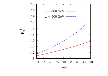
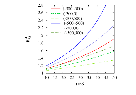
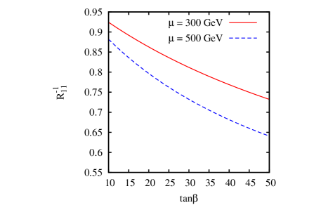
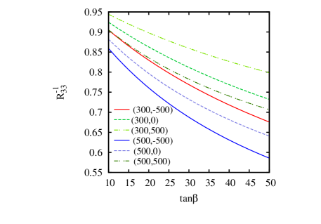
Figure 1: Dependence of the general couplings $R^{-1}_{ii}$ on $tan\beta$ in the exemplary case of the MSSM for various values of the higgsino mass parameter $\mu$ and the up-type trilinear coupling $A$. The left-hand plots are for $R^{-1}_{11}=R^{-1}_{22}$, while those on the right are for $R_{33}^{-1}$. We present the case of negative $\mu$ in the top panels and for positive $\mu$ below. The other SUSY parameters are $M_{\tilde{g}}$ = 800 GeV and $M_{\tilde{b}_{1}}=M_{\tilde{t}_{1}}=500$ GeV. We have also assumed $M_{\tilde{t}_{L}}=M_{\tilde{t}_{R}}$ and $M_{\tilde{b}_{L}}=M_{\tilde{b}_{R}}$. The legends in the right top and right bottom panels correspond to $(\mu,A)$ in GeV.

III Charged Higgs at the LHC

As argued above, at the LHC we can observe the vertex $b-t-H^{\pm}$ by producing a charged Higgs boson. In the large $\tan\beta$ region of the parameter space, the charged Higgs boson will be predominantly produced through the partonic process $gb\to tH^{\pm}$. The effective interaction term of the charged Higgs boson with $t$ and $b$ quarks in the 2HDMs, that can be probed at the LHC, can be written as:

$${\cal L} = \frac{g}{2\sqrt{2}\;m_{W}}V_{tb}H^{+}{\bar{t}}\left(m_{t}\cot\beta(1-\gamma_{5})+m_{b}R_{33}^{-1}\tan\beta(1+\gamma_{5})\right)b+h.c.\,\,\,.$$ (3)

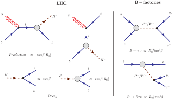
Figure 2: Production and decay of a charged Higgs boson at the LHC involving the general third-generation coupling $R_{33}^{-1}$ (left) and (semi-)leptonic $B$-decays involving the general first- and second-generation couplings $R_{11}^{-1}$ and $R_{22}^{-1}$.

The cross-section for $gb\rightarrow tH^{\pm}$ (see the left-hand portion of Fig. 2) can be written as:

$$\sigma(gb\rightarrow tH^{\pm})\propto\left(m^{2}_{t}\cot^{2}\beta+m^{2}_{b}(R^{-1}_{33})^{2}\tan^{2}\beta\right)\,\,\,.$$ (4)

In the large $\tan\beta$-region of the parameter space, the decay width for a charged Higgs boson is dominated by the channels $H^{\pm}\to\tau\nu$ and $H^{\pm}\to tb$, whose decay widths in the large $\tan\beta$ region can be written as:

$$\Gamma(H^{-}\to\tau^{-}\nu_{\tau}) \simeq \frac{m_{H^{\pm}}}{8\pi v^{2}}m_{\tau}^{2}\tan^{2}\beta\left(1-\frac{m_{\tau}^{2}}{m_{H^{\pm}}^{2}}\right)^{2}\,\,\,,$$ (5)

$$\Gamma(H^{-}\to{\bar{t}}b) \simeq \frac{3\;m_{H^{\pm}}}{8\;\pi v^{2}}\ m_{b}^{2}(R^{-1}_{33})^{2}\tan^{2}\beta\left(1-\frac{m_{t}^{2}}{m_{H^{\pm}}^{2}}-\frac{m_{b}^{2}}{m_{H^{\pm}}^{2}}\right)$$ (6)

$$\hskip 56.9055pt\times\left[1-\left(\frac{m_{t}+m_{b}}{m_{H^{\pm}}}\right)^{2}\right]^{1/2}\left[1-\left(\frac{m_{t}-m_{b}}{m_{H^{\pm}}}\right)^{2}\right]^{1/2}\,\,\,.$$

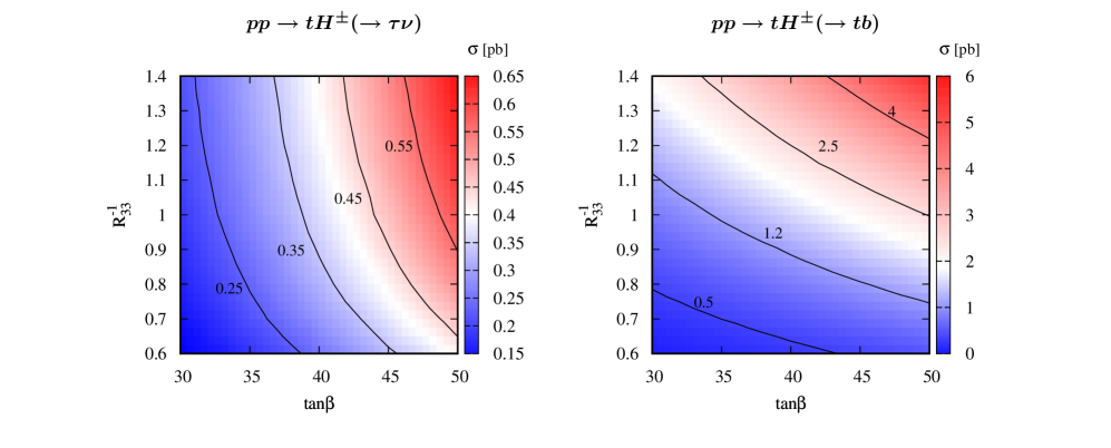
Figure 3: Contour plots of the cross-sections for the processes $pp\to tH^{\pm}(\to\tau\nu)$ (left) and $pp\to tH^{\pm}(\to tb)$ (right) versus $R^{-1}_{33}$ and $tan\beta$ with fixed $m_{H^{\pm}}=$ 300 GeV.

For the main production mechanism ($gb\to tH^{\pm}$) considered here, we simulated the leading order (LO) cross-sections using the pythia Monte Carlo generator Sjostrand:2006za and cteq6l1 parton densities Nadolsky:2008zw using LHAPDF Whalley:2005nh . The renormalisation and factorisation scales $\mu_{R}$ and $\mu_{F}$ were identified with the average mass of the two final state particles. It is well known that the process $gg\to tbH^{\pm}$, although formally of next-to-leading order (NLO), is numerically important due to the enhanced splitting of gluons into collinear bottom-antibottom pairs. In our simulations this process was taken into account following the ideas originally proposed in the late 80’s in Ref. Barnett:1987jw , using the matchig Alwall:2005gs addition to pythia6.4.11 Sjostrand:2006za , which then allowed for a better description of hard additional jets and at the same time for a consistent subtraction of the mass logarithm coming from the overlap with the LO process Alwall:2005gs . However, since the matched sum is still normalised to the LO total cross-section, we renormalise it to NLO precision using cteq6m parton densities and the corresponding value of $\lambda_{\overline{\rm MS}}^{n_{f}=5}=226$ MeV in the computations given in Ref. Plehn:2002vy ; Berger:2003sm , which has been shown to be in good agreement with the one performed in Ref. Zhu:2001nt . For a Higgs boson mass of 300 GeV and in the $\tan\beta$ region of 30–50 considered here, the correction varies very little and can be well approximated with a constant factor of $1.2$.

In Fig. 3 we show contour plots of the cross-sections at the LHC in the $R_{33}^{-1}-\tan\beta$ plane. It is evident from these plots and Eqs. (4), (5) and (6) that a measurement of the ratio of these cross-sections could give us a measurement of $R_{33}^{-1}$ and thus constrain the parameter space of any new particles contributing to its loop corrections. The ratio will also be relatively free from the theoretical uncertainty arising at the production level of the charged Higgs boson. In principle, by measuring these cross-sections simultaneously, one can estimate $R_{33}^{-1}$ and $\tan\beta$. We shall demonstrate this in an upcoming work using detailed simulations future .

IV Charged Higgs and tauonic $B$-decays

The first measurement of tauonic $B$-decays was done by the L3 collaboration at LEP Acciarri:1994hb , where they measured the inclusive branching fraction of tauonic $B$-decays, namely $B\to X\tau\nu$. Based on the LEP measurement of inclusive tauonic decays, Grossman et al. Grossman:1994ax obtained the limits on $\tan\beta$ as $\tan\beta<0.52(m_{H}/1GeV)$. The tauonic $B$-decays can be mediated by tree level charged Higgs boson exchanges and could be very sensitive to charged Higgs boson couplings Itoh:2004ye ; Kiers:1997zt ; Nierste:2008qe ; Hou:1992sy ; Tanaka:1994ay . In Fig. 2 we have shown the Feynman diagrams contributing to these decays. The importance of purely tauonic $B$-decays ($B\to\tau\nu$) in constraining charged Higgs properties was pointed out in Ref. Hou:1992sy . The exclusive tauonic decay $B\to D\tau\nu$ offers many more kinematical distributions Tanaka:1994ay that could further help in pinning down the structure of the effective Hamiltonian responsible for these decays. In Ref. Itoh:2004ye it was shown that considering both these decay modes, namely $B\to\tau\nu$ and $B\to D\tau\nu$, could possibly give a two fold ambiguity in measuring $\tan\beta/m_{H}$. But by combining these measurements one can possibly remove this two fold ambiguity. Using the effective vertices given in Eq. (1) and shown in Fig. 2 (right), the rates of the $B\to\tau\nu$ and $B\to D\tau\nu$ processes can be written as functions of the parameters $\tan\beta$ and $m_{H^{\pm}}$ and the loop correction factors as:

$$Br(B\to\tau\nu) \propto \left[a+b\frac{\tan^{2}\beta(R^{-1}_{11})^{2}}{m_{H^{\pm}}^{2}}\right]^{2}\,\,\,,$$ (7)

$$Br(B\to D\tau\nu) \propto a^{\prime}+b^{\prime}\frac{\tan^{2}\beta(R^{-1}_{22})^{2}}{m_{H^{\pm}}^{2}}+c^{\prime}\left(\frac{\tan^{2}\beta(R^{-1}_{22})^{2}}{m_{H^{\pm}}^{2}}\right)^{2}\,\,\,,$$ (8)

where $a,b,a^{\prime},b^{\prime}$ and $c^{\prime}$ are factors that do not depend on any new physics parameters. In writing Eqs. (7) and (8) we have used the matrix elements as given in Refs. Itoh:2004ye ; Gorbahn:2009pp ; Kiers:1997zt . The coefficients $a^{\prime},b^{\prime},c^{\prime}$ depend on the form factors for the $B\to D$ transition. Presently these form factors have substantial theoretical uncertainties which can be translated into theoretical errors on the branching ratios of these modes. For our illustrative purposes we have used the prescription of the form factors for $B\to D$ transition as given in Ref. Gorbahn:2009pp . Gorbahn et al. Gorbahn:2009pp have also estimated the possible theoretical uncertainties on the form-factors for $B\to D$ transitions.

V Effective couplings determination

We have discussed in sections III and IV the phenomenology of a charged Higgs boson at the LHC and at $B$-factories for large values of $\tan\beta$ in relation to the study of its couplings. In the following we give the results of our numerical study and in particular of the possibility of combining these two kinds of complementary experimental results in order to constrain the charged Higgs coupling.

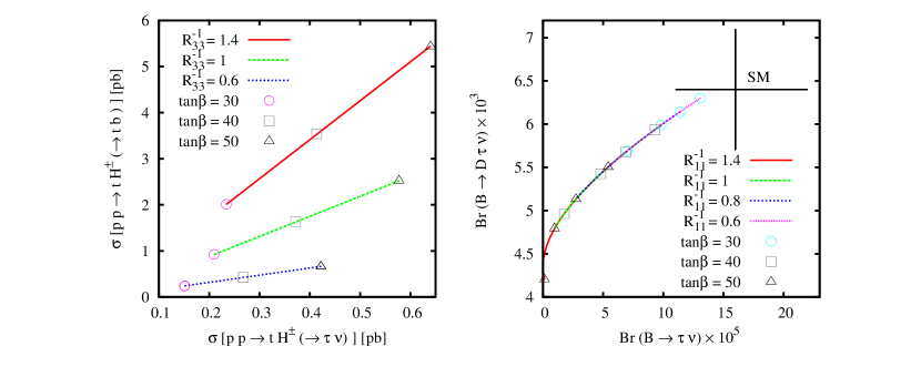
Figure 4: Correlation plots of the cross-sections for the processes $pp\to t(b)H^{\pm}(\to\tau\nu)$ and $pp\to t(b)H^{\pm}(\to tb)$ for three values of $R^{-1}_{33}$ and $tan\beta$ (left) and of the branching ratios for $B\to D\tau\nu$ and $B\to\tau\nu$ (right) for various values of $tan\beta$ and $\widehat{R}_{d}^{-1}$ with fixed $m_{H^{\pm}}=300$ GeV.

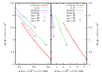
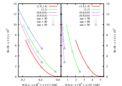
Figure 5: Correlation plots of the branching ratio $B\to D\tau\nu$ with the cross-sections $\sigma(pp\to tH^{\pm}(\to\tau\nu))$ (top left) and $\sigma(pp\to tH^{\pm}(\to tb))$ (top right) and of the branching ratio $B\to\tau\nu$ with the cross-sections $\sigma(pp\to tH^{\pm}(\to\tau\nu))$ (bottom left) and $\sigma(pp\to tH^{\pm}(\to tb))$ (bottom right) for various values of $tan\beta$ and $\widehat{R}_{d}^{-1}$. The numbers in the legend refer to $(R_{11}^{-1},R_{33}^{-1})$.

In Figs. 4 and 5 we have plotted the correlations amongst the four processes (two from the LHC and two from $B$-factories) considered here. In these plots we have varied $\tan\beta$ in the range $30<\tan\beta<50$ for different values of $R_{ii}^{-1}$ ($ii=11,33$). The left panel of Fig. 4 shows the correlation of the LHC observables, whilst the correlation of $B$-decay branching ratios in the right panel of Fig. 4 gives the same line for different values of $R_{11}^{-1}$. The reason for this can be seen from the Feynman diagrams given in Fig. 2 where $R_{ii}^{-1}$ and $\tan\beta$ arise from the same combination ($\equiv R_{ii}^{-1}\tan^{2}\beta$) in the tauonic $B$-decays considered in this work. Hence the measurement of these two $B$-decays will only give an estimate of the product of $R_{11}^{-1}$ and $\tan\beta$. However, by considering the correlations of the $B$-decay observables with LHC observables, as shown in Fig. 5, one can remove this degeneracy. So in principle it is possible to measure the four parameters ($\tan\beta$ and $R_{ii}^{-1}$ with $ii=11,22,33$) using the six correlation plots shown in Figs. 4 and 5. We will now demonstrate this statement by considering an illustrative set of input parameters.

The illustrative point we have chosen lies at $\tan\beta=40$, $m_{H^{\pm}}=300$ GeV and $R_{33}^{-1}=1$. For this illustrative point we first start by summarising our simulation results for the charged Higgs boson production and decay in the $H^{\pm}\to\tau\nu$ mode. As mentioned earlier, this simulation was carried out using matchig Alwall:2005gs so as to include all the relevant processes in pythia 6.4.11 Sjostrand:2006za . In these simulations the charged Higgs boson is allowed to decay via the channel $H^{\pm}\to\tau^{had}\nu$. The events thus generated were further passed through the fast detector simulator atlfast atlfast . atlfast identifies isolated leptons, $b$ and $\tau$ jets. It also reconstructs missing energy. The jets in atlfast are reconstructed using simple cone algorithms. The decay chain we have used is Assamagan:2002ne ; Hashemi:2008ma ; cms:taunu ; Mohn:2007fd :

$$pp\to t(\to jjb)(b)H(\to\tau\nu)\to jjb(b)\tau\not\!\!E_{T}$$

For the analysis we have used following pre-selection cuts:

• The event should have exactly one $\tau$-jet with $p_{T}^{\tau}>40$ GeV.

• There should be at least three light jets with $p_{T}>30$ GeV. At least one of these jets must be a $b$-jet.

In order to reduce the backgrounds we have in addition used the following selection cuts Assamagan:2002ne ; Hashemi:2008ma ; cms:taunu ; Mohn:2007fd :

• ${\cal N}_{1}$ : $p_{T}^{\tau}>100$ GeV. This reduces the backgrounds where $\tau$ comes from a decay of the $W$-boson. This cut is too severe for a light charged Higgs but there is no substantial reduction in event rates for the signal as we have considered a relatively heavy Higgs.

• ${\cal N}_{2}$ : $\not\!\!E_{T}>100$ GeV. This cut again reduces SM backgrounds with neutrinos in the final state.

• ${\cal N}_{3}$ :$\triangle\phi>1$ radian, where $\triangle\phi$ is the azimuthal angle between the $\tau$-jet and $\not\!\!p_{T}$.

The uncertainty in cross-section measurements is estimated as Assamagan:2002ne :

$$\frac{\triangle(\sigma\times BR)}{(\sigma\times BR)}=\sqrt{\frac{S+B}{S^{2}}}$$

where $S$ and $B$ are signal and background events respectively.

The numerical results of our analysis are summarized in Table 1. The table shows that for a reasonable range of input parameters the cross-sections at the LHC can be measured with a 10% accuracy for a luminosity of ${\cal L}$ = 100 fb^-1, whereas the measurement can be improved substantially for higher luminosities. Note that the error in the measurement of $\tan\beta$ is consistent with the observations made in Ref. Assamagan:2002ne . For our analysis we have taken the error in the measurement of the cross-section in this channel to be 10% for a luminosity of 100 fb^-1 and 7.5% for a luminosity of 300 fb^-1. At this point we would like to note that for our results we have used fast detector simulator atlfast atlfast and have followed the methodology as given in Ref. Assamagan:2002ne . In our work instead of using pythia to consider the dominant partonic process $gb\to tH^{\pm}$ (as was done in Ref. Assamagan:2002ne ) we have used matchig Alwall:2005gs in addition to pythia to include the additional sub-processes namely $gg\to tbH^{\pm}$ and $q\bar{q}\to tbH^{\pm}$. In a realistic simulation with full detector simulator the errors in cross-section measurements could be a bit larger. As mentioned, our results are consistent with the earlier studies Assamagan:2002ne and the recent studies done in Refs. cms:taunu ; Mohn:2007fd with fast detector simulators. Mohn et al. Mohn:2007fd also proposed some additional set of cuts like the transverse momentum ratio of $\tau$-jet and hardest parton jet that has been used for top-reconstruction. This further improves the discovery reach of charged Higgs boson in $H^{\pm}\to\tau\nu$ mode. But these studies assumed tree level Universal coupling of charged Higgs bosons to quarks.

Table 1: Cumulative Efficiencies of cuts and estimated errors for measurements of a signal cross-section for the process $pp\to t(b)H(\to\tau^{had}\nu)$. For these numbers we have fixed $m_{H^{\pm}}=300$ GeV.

	$R_{33}^{-1}$ = 0.7	$R_{33}^{-1}$ = 1	$R_{33}^{-1}$ = 1.3
$\sigma$ (fb)	204	249	273
Pre-selection	48 $\times 10^{-3}$	48 $\times 10^{-3}$	48 $\times 10^{-3}$
${\cal N}_{1}$	$12.8\times 10^{-3}$	$13\times 10^{-3}$	$13\times 10^{-3}$
${\cal N}_{2}$	$61\times 10^{-4}$	$67\times 10^{-4}$	$66\times 10^{-4}$
${\cal N}_{3}$	$47\times 10^{-4}$	$53\times 10^{-4}$	$52\times 10^{-4}$
$\triangle(\sigma\times BR)/(\sigma\times BR)$ (${\cal L}=100fb^{-1}$)	10.6 $\%$	9.5 $\%$	8.6 $\%$
$\triangle(\sigma\times BR)/(\sigma\times BR)$ (${\cal L}=300fb^{-1}$)	6.2 $\%$	5.5 $\%$	5 $\%$

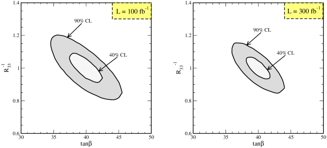
Figure 6: $\chi^{2}$ contours for 100 fb^-1 (left panel) and 300 fb^-1 (right panel) luminosities with input values $R_{33}^{-1}=1$ and $\tan\beta=40$.

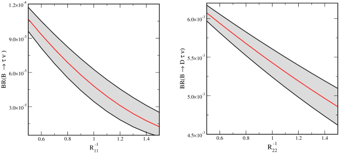
Figure 7: Branching ratios of $B\to\tau\nu$ (left) and $B\to D\tau\nu$ (right) as a function of $R_{11}^{-1}$ and $R_{22}^{-1}$, respectively. The shaded area corresponds to $tan\beta$ in the range $37<tan\beta<43$.

For the other dominant decay mode of the charged Higgs boson, namely $H^{\pm}\to tb$, the cross-section times branching ratio is much larger than for $H^{\pm}\to\tau\nu$. However, this mode has at least three $b$-jets in its final state. To detect a charged Higgs boson in this mode one has to tag all the final state $b$-jets, which reduces the efficiency of this mode. In this mode one therefore has to reconstruct the two top-quark candidates in order to reconstruct a charged Higgs boson by using the invariant mass $m_{tb}$. The combinatorial backgrounds associated with $t\bar{t}$ production makes the observation of this channel a challenging task Assamagan:2002ne . For this reason the $H^{\pm}\to tb$ channel may not be a good discovery channel for a charged Higgs boson at the LHC. ATLAS Assamagan:2002ne ; Potter:2008zza and CMS cms:tb studies for a discovery of the charged Higgs boson using this decay mode indicate that, although it is possible to observe the charged Higgs boson in this mode, the most optimistic scenario for the discovery of a charged Higgs boson at the LHC in the large $\tan\beta$ parameter space is through the decay $H^{\pm}\to\tau\nu$ Hashemi:2008ma ; Mohn:2007fd ; cms:taunu ; Potter:2008zza ; Assamagan:2002ne . However, as argued in Ref. Assamagan:2002ne , the significance of this channel improves if one has a prior estimation of the mass of the charged Higgs boson. It was emphasised in Ref. Assamagan:2002ne that the channel ($H^{\pm}\to tb$) could be a useful channel to probe the charged Higgs boson for a low charged Higgs boson mass (up to a charged Higgs boson mass of 300 GeV) in a relatively low $\tan\beta$ region ($\tan\beta<2.5$). For high $\tan\beta$ ($>25$), the charged Higgs boson can be probed in this channel for a fairly high charged Higgs-boson mass. The detection of a heavy charged Higgs boson in this mode is possible because we can have a hard $b$-jet in the final state that can help in optimising the cuts, and hence improving the efficiency. For our analysis we have taken the accuracy of the cross-section in this channel, that is, the error in the measurement of the $pp\to tH^{\pm}(\to tb)$ cross-section to be 15% for a luminosity of 100 fb^-1 and 12% for a luminosity of 300 fb^-1.

VI Discussion and conclusions

By measuring the cross-sections of the two decay modes of the charged Higgs boson at the LHC we discussed in the previous section, one can determine the charged Higgs boson couplings. Assuming the charged Higgs boson mass to be known (taken to be 300 GeV in our present analysis) we have tried to do a $\chi^{2}$ fit in the $R_{33}^{-1}$ - $\tan\beta$ plane using the cross-section measurement uncertainties as given in Table 1 and at the end of the previous section. The results are presented in Fig. 6. As can be seen from these figures, it might be possible to measure $R^{-1}_{33}$ and $\tan\beta$ with an accuracy of about 10% at high luminosity. Armed with this information about $\tan\beta$, from the LHC measurements, it can then be taken as an input to the $B$-decay measurements, namely $B\to\tau\nu$ and $B\to D\tau\nu$. In Fig. 7 we have plotted the respective branching ratios of the $B$-decays as a function of $R_{11}^{-1}$ and $R_{22}^{-1}$. The shaded area in this figure corresponds to a 10% error in $\tan\beta$ around the central value of 40. Future Super-$B$ factories are expected to measure the $B\to\tau\nu$ and $B\to D\tau\nu$ to a precision of 4% and 2.5% respectively Browder:2007gg . The present world average experimental results for tauonic $B$-decays are $BR(B\to\tau\nu)=(1.51\pm 0.33)\times 10^{-4}$ and $BR(B\to D\tau\nu)/BR(B\to D\mu\nu)=(41.6\pm 11.7\pm 5.2)\%$ Aubert:2007dsa ; Browder:2007gg . Presently if one uses UTfit prescription of $|V_{ub}|$ then there is substantial disagreement between experimental and SM estimates for the branching fractions of $B\to\tau\nu$. However, the PDG value of $|V_{ub}|$ is much higher than the value given by UTfit. The main source of this problem is the large difference in the inclusive and exclusive estimation of $|V_{ub}|$ Lunghi:2009ke . Recently, proposals have been given in Ref. Lunghi:2009ke to reduce this tension between experimental and theoretical SM values of $B\to\tau\nu$. To sum up the present theoretical uncertainties in $BR(B\to\tau\nu)$ and $BR(B\to D\tau\nu)$ there is still a large discrepancy due to $f_{B}$, $|V_{ub}|$ and semi-leptonic form factors, where it may be possible to reduce these uncertainties to a 5% level in the future bfuture . Transforming the improved projected theoretical information of these decays along with future Super-$B$ factory measurements in Fig. 7 one can measure $R_{11}^{-1}$ and $R_{22}^{-1}$ to a fairly high precision.

To summarise, we have tried to demonstrate that at the LHC alone it is possible to measure the charged Higgs boson couplings, namely $\tan\beta$ and $R^{-1}_{33}$, to an accuracy of less than 10%. Combining this information from the LHC with improved $B$-factory measurements, one can measure all four observables indicated in the introduction. These observables represent effective couplings of a charged Higgs boson to the bottom quark and the three generations of up-type quarks, thus demonstrating that it is possible to perform a universality test of the charged Higgs boson couplings to quarks by the combination of low energy measurements at future Super-$B$ factories and charged Higgs boson production at the LHC.

References

- (1) B. Aubert et al. [BABAR Collaboration], Phys. Rev. Lett. 100, 021801 (2008); B. Aubert et al. [BABAR Collaboration], Phys. Rev. D 79, 092002 (2009); A. Matyja et al. [Belle Collaboration], Phys. Rev. Lett. 99, 191807 (2007).
- (2) K. Ikado et al., Phys. Rev. Lett. 97, 251802 (2006); B. Aubert et al. [BABAR Collaboration], Phys. Rev. D 77, 011107 (2008); B. Aubert et al. [BABAR Collaboration], Phys. Rev. D 76, 052002 (2007).
- (3) K. A. Assamagan, Y. Coadou and A. Deandrea, Eur. Phys. J. direct C 4, 9 (2002); K. A. Assamagan, Acta Phys. Polon. B 31, 863 (2000); K. A. Assamagan and Y. Coadou, Acta Phys. Polon. B 33, 707 (2002).
- (4) M. Hashemi, S. Heinemeyer, R. Kinnunen, A. Nikitenko and G. Weiglein, arXiv:0804.1228 [hep-ph] ; S. Heinemeyer, A. Nikitenko and G. Weiglein, AIP Conf. Proc. 1078, 204 (2009).
- (5) B. Mohn, M. Flechl and J. Alwall, ATL-PHYS-PUB-2007-006 ;
- (6) P. Salmi, R. Kinnunen and N. Stepanov, CMS NOTE 2002/024 [arXiv:hep-ph/0301166]; S. Lowette, J. Heyninek and P. Vanlaer, CMS NOTE 2008/017.
- (7) R. Kinnunen CMS NOTE 2006/100; CMS TDR, CERN/LHCC 2006-021.
- (8) C. Potter, AIP Conf. Proc. 1078, 201 (2009) ; ATLAS Coll., CERN-OPEN-2008-020.
- (9) L. J. Hall, R. Rattazzi and U. Sarid, Phys. Rev. D 50, 7048 (1994).
- (10) H. Itoh, S. Komine and Y. Okada, Prog. Theor. Phys. 114, 179 (2005).
- (11) M. S. Carena, D. Garcia, U. Nierste and C. E. M. Wagner, Nucl. Phys. B 577, 88 (2000).
- (12) M. Gorbahn, S. Jäger, U. Nierste and S. Trine, arXiv:0901.2065 [hep-ph].
- (13) T. Blazek, S. Raby and S. Pokorski, Phys. Rev. D 52, 4151 (1995).
- (14) A. Dedes and A. Pilaftsis, Phys. Rev. D 67, 015012 (2003) [arXiv:hep-ph/0209306].
- (15) G. D’Ambrosio, G. F. Giudice, G. Isidori and A. Strumia, Nucl. Phys. B 645, 155 (2002) [arXiv:hep-ph/0207036].
- (16) A. J. Buras, P. H. Chankowski, J. Rosiek and L. Slawianowska, Nucl. Phys. B 659, 3 (2003) [arXiv:hep-ph/0210145].
- (17) K. S. Babu and C. F. Kolda, Phys. Rev. Lett. 84, 228 (2000); S. R. Choudhury and N. Gaur, Phys. Lett. B 451, 86 (1999) [arXiv:hep-ph/9810307]; M. S. Carena, D. Garcia, U. Nierste and C. E. M. Wagner, Phys. Lett. B 499, 141 (2001); A. J. Buras, P. H. Chankowski, J. Rosiek and L. Slawianowska, Nucl. Phys. B 619, 434 (2001); A. J. Buras, P. H. Chankowski, J. Rosiek and L. Slawianowska, Phys. Lett. B 546, 96 (2002); A. J. Buras, P. H. Chankowski, J. Rosiek and L. Slawianowska, Nucl. Phys. B 659, 3 (2003); M. S. Carena, A. Menon, R. Noriega-Papaqui, A. Szynkman and C. E. M. Wagner, Phys. Rev. D 74, 015009 (2006).
- (18) T. Sjöstrand, S. Mrenna and P. Skands, JHEP 0605, 026 (2006).
- (19) P. M. Nadolsky et al., Phys. Rev. D 78, 013004 (2008).
- (20) M. R. Whalley, D. Bourilkov and R. C. Group, arXiv:hep-ph/0508110.
- (21) J. Alwall, arXiv:hep-ph/0503124.
- (22) T. Plehn, Phys. Rev. D 67, 014018 (2003).
- (23) R. M. Barnett, H. E. Haber and D. E. Soper, Nucl. Phys. B 306, 697 (1988) ; D. A. Dicus and S. Willenbrock, Phys. Rev. D 39, 751 (1989).
- (24) E. L. Berger, T. Han, J. Jiang and T. Plehn, Phys. Rev. D 71, 115012 (2005).
- (25) S. H. Zhu, Phys. Rev. D 67 075006 (2003).
- (26) A. S. Cornell, A. Deandrea, N. Gaur, H. Itoh, M. Klasen, Y. Okada, work in progress.
- (27) M. Acciarri et al. [L3 Collaboration], Phys. Lett. B 332, 201 (1994).
- (28) Y. Grossman and Z. Ligeti, Phys. Lett. B 332, 373 (1994) [arXiv:hep-ph/9403376] ; Y. Grossman, H. E. Haber and Y. Nir, Phys. Lett. B 357, 630 (1995) [arXiv:hep-ph/9507213]; Y. Grossman and Z. Ligeti, Phys. Lett. B 347, 399 (1995) [arXiv:hep-ph/9409418].
- (29) K. Kiers and A. Soni, Phys. Rev. D 56, 5786 (1997).
- (30) U. Nierste, S. Trine and S. Westhoff, Phys. Rev. D 78, 015006 (2008); S. Trine, arXiv:0810.3633 [hep-ph].
- (31) M. Tanaka, Z. Phys. C 67, 321 (1995) [arXiv:hep-ph/9411405]; G. H. Wu, K. Kiers and J. N. Ng, Phys. Lett. B 402, 159 (1997) [arXiv:hep-ph/9701293] ; G. H. Wu, K. Kiers and J. N. Ng, Phys. Rev. D 56, 5413 (1997) [arXiv:hep-ph/9705293].
- (32) W. S. Hou, Phys. Rev. D 48, 2342 (1993) ; A. G. Akeroyd and S. Recksiegel, J. Phys. G 29, 2311 (2003) [arXiv:hep-ph/0306037].
- (33) E. Richter-Was et al. , ATLFAST 2.2: A fast simulation package for ATLAS, ATL-PHYS-98-131.
- (34) T. Browder, M. Ciuchini, T. Gershon, M. Hazumi, T. Hurth, Y. Okada and A. Stocchi, JHEP 0802, 110 (2008); M. Bona et al., arXiv:0709.0451 [hep-ex]; T. Iijima, Search for charged Higgs in and decays, talk given at the workshop on “Hints for new physics in flavor decays”, Tsukuba, Japan (2009).
- (35) E. Lunghi and A. Soni, arXiv:0912.0002 [hep-ph]; W. Altmannshofer, A. J. Buras, S. Gori, P. Paradisi and D. M. Straub, arXiv:0909.1333 [hep-ph].
- (36) M. Ciuchini, UTfit: status and perspectives, talk given at the second workshop on “Theory, phenomenology and experiments in heavy flavor physics”, Capri, Italy (2008); M. Artuso et al., Eur. Phys. J. C 57, 309 (2008).