Möbius Graphene Strip as Topological Insulator

Abstract

We study the electronic properties of Möbius graphene strip with a zigzag edge. We show that such graphene strip behaves as a topological insulator with a gapped bulk and a robust metallic surface, which enjoys some features due to its nontrivial topology of the spatial configuration, such as the existence of edge states and the non-Abelian induced gauge field. We predict that the topological properties of the Möbius graphene strip can be experimentally displayed by the destructive interference in the transmission spectrum, and the robustness of edge states under certain perturbations.

I INTRODUCTION

Because of the unusual properties and potential applications, topological insulators have recently been under great focus both experimentally topo01 ; topo02 and theoretically topo1 ; topo2 ; topo3 ; topo4 ; topo5 ; topo6 ; topo7 . The topological insulator system belongs to a novel category, possessing an insulating bulk, with a gap in the energy spectrum of propagating electrons, whereas its surface is metallic. The edge states promise such metallic feature and describe the electrons localized on the surface with energy levels lying just within the gap of the bulk topo1 . For many systems in this category, the surfaces are no longer conductive when some perturbations are applied. However, for some system with nontrivial topology, the edge states are robust under perturbations. Such systems with robust metallic surfaces are referred to as topological insulators topo1 .

It is natural to imagine that those topological features of electrons can be realized through nontrivial topology in the configuration space of the system considered. A most recent illustration is the tight binding model for electrons hopping on a Möbius ladder Moladder1 . In this investigation, observable effects of Möbius boundary condition were found for a finite lattice. Destructive interference emerges from the transmission spectrum to display the typical topological feature. It was proved that such destructive interference can be explained in terms of a non-Abelian gauge field induced by the nontrivial topology. However, such a novel nanostructure can not be regarded as a topological insulator, because this quasi-1D system has no edge states.

In this paper, we study the electronic properties of a Möbius graphene strip. We show that with a 2D nontrivial topological structure, the Möbius graphene strip Mobius1 ; Mobius2 ; Mobius3 ; Mobius4 ; Mobius5 ; Mobius6 with zigzag edges (see Fig. 1(b)) behaves as a typical topological insulator since it possesses robust edge states. It is noticed that there is no edge state in such Möbius strip with an armchair edge, thus no such nontrivial topological properties appear. Our investigation will focus on the situation with a zigzag edge. Through analytic approaches, we first predict that the robustness of the edge states is maintained under perturbation with uniform electric field in our discussion. And we compare the Möbius graphene strip with a generic one whose edges turn to be insulators in the same electric field. Besides, destructive interference in the transmission spectrum is found in the Möbius graphene strip, which is caused by the non-Abelian gauge field. Based on this observation, we propose a possible approach of quantum manipulation on the transport properties of the Möbius graphene strip through a magnetic flux.

Figure 1: (color online) (a) A zigzag graphene strip is schematically illustrated in a 2D version with open boundary condition along $y$ direction. The white (black) dots represent sublattice A (B). The 3D version of the graphene strip with Möbius boundary condition along the $x$ direction ($\psi_{a(b)}(\mathbf{r})=\psi_{b(a)}(\mathbf{\widetilde{r}}+L\mathbf{e_{x}})$, where $\mathbf{r}=(x,y)$ and $\widetilde{\mathbf{r}}=(x,-y)$) and periodic boundary condition ($\psi_{a(b)}(\mathbf{r})=\psi_{a(b)}(\mathbf{r}+L\mathbf{e_{x}})$) are plotted in (b) and (c), respectively.

This paper is arranged as follows. In Sec. II, we give an analytical description of the edge states for the generic and Möbius graphene strip. Here the tight binding Hamiltonian is used to model the graphene strip with finite width. In Sec. III, a uniform electric field is applied to the generic and Möbius graphene strip as a perturbation. We compare the energy bands of the edge states in the generic and Möbius graphene strips under the uniform electric field. Robustness of the edge states in the Möbius graphene strip under such perturbation is demonstrated. And we prove the candidacy of Möbius graphene strip as a topological insulator. Additionally, in Sec. IV, we discuss the topology-induced non-Abelian gauge field in the Möbius graphene strip and its observable effects in future experiments. Besides, we propose a possible quantum manipulation mechanism upon the Möbius graphene strip through a magnetic flux. Finally, the conclusion is presented in Sec. V.

II EDGE STATES IN MÖBIUS GRAPHENE STRIP

To describe the motion of electrons of graphene, we use the tight binding model Carbon1 ; Carbon2 ,

$$H=-J\sum_{\left\langle i,j\right\rangle}[\psi_{a}^{\dagger}(\mathbf{\mathbf{r_{i}}})\psi_{b}(\mathbf{r_{j}})+H.c.],$$ (1)

where $\psi_{a}(\mathbf{r_{i}})$($\psi_{b}(\mathbf{r_{i}})$) annihilates an electron on site $\mathbf{r_{i}}$ of sublattice A(B), and the sum is taken over the nearest neighbor sites $\left\langle i,j\right\rangle$ with corresponding hopping constant $J$. For the zigzag graphene strip with finite width ($N$ regular hexagons in Fig. 1(a)) along $y$ direction, the $y$ component of the spacial vector $\mathbf{r}$ for A and B sublattices only take a finite number of values, e.g., $y_{m}^{(a)}=[3(N-m)-1]l/2$ for sublattice A, and $y_{m}^{(b)}=[3(N-m)-2]l/2$ for sublattice B. Here, $l$ is the distance between nearest neighbors in the lattice, and $m=0,1,...,2N-1$. Usually, it is assumed that the length of the graphene strip ($M$ regular hexagons along x direction, as in Fig. 1(a)) is much larger than the width, namely, $M\gg N$, and periodic boundary condition is taken as

$$\psi_{a(b)}(\mathbf{r})=\psi_{a(b)}(\mathbf{r}+L\mathbf{e_{x}}),$$ (2)

with $L=\sqrt{3}Ml.$ Thus, it is proper to perform Fourier transformation only for the $x$ component of $\mathbf{r}$ upon the field operators of electrons as

$$\psi_{a(b)}(k_{x},y)=\frac{1}{\sqrt{M}}\sum_{x}\psi_{a(b)}(x,y)e^{-ik_{x}x},$$ (3)

and $k_{x}$ can be considered as continuous since $L$ is large enough.

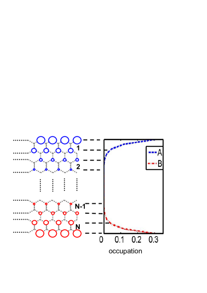
Figure 2: (color online) On the left is the schematic illustration of the on-site electron occupation of an edge state with $k_{x}=1.2\pi/d$, $d=\sqrt{3}l$, in which the size of each circle represents the magnitude of the electron occupation on that lattice site. And the right figure displays the corresponding values of electron occupation on sublattice A (blue circles) and B (red circles) respectively.

For a zigzag graphene strip, there exist eigenstates strongly localized on the edges of the strip with their energies lying exactly within the gap  edgestate1 ; edgestate2 ; edgestate3 ; edgestate4 , which are called edge states. A straightforward calculation gives approximate edge states

$$\left|\Psi_{\pm}(k_{x})\right\rangle=D_{e\pm}^{\dagger}(k_{x})\left|vac\right\rangle,$$ (4)

which are defined by the corresponding annihilation operators

$$D_{e\pm}(k_{x})=\frac{1}{\sqrt{2}}[A_{e}(k_{x})\pm B_{e}(k_{x})],$$ (5)

where the collective operators

$$A_{e}(k_{x})= \frac{1}{\sqrt{S_{k_{x}}}}\sum_{m=0}^{2N-1}p_{k_{x}}^{m}\psi_{a}(k_{x},y_{m}^{(a)}),$$ (6a)

$$B_{e}(k_{x})= \frac{1}{\sqrt{S_{k_{x}}}}\sum_{m=0}^{2N-1}p_{k_{x}}^{2N-1-m}\psi_{b}(k_{x},y_{m}^{(b)})$$ (6b)

respectively represent parts of the edge states localized on the edges, as shown in Fig. 2. Here,

$$p_{k_{x}}=-2\cos\left(\frac{\sqrt{3}k_{x}l}{2}\right)$$ (7)

represents the decay rate of the single electron on-site occupation probability along $y$ direction. And

$$S_{k_{x}}=\frac{1-p_{k_{x}}^{4N}}{1-p_{k_{x}}^{2}}$$ (8)

is the normalization constant. $\left|\Psi_{\pm}(k_{x})\right\rangle$ are the anti-bond and bond states with respect to the states $A_{e}^{\dagger}(k_{x})\left|vac\right\rangle$ and $B_{e}^{\dagger}(k_{x})\left|vac\right\rangle$. They correspond to the eigenenergy

$$E_{e\pm}(k_{x})=\pm J\frac{p_{k_{x}}^{2N}(1-p_{k_{x}}^{2})}{1-p_{k_{x}}^{4N}}.$$ (9)

Actually, only when $|p_{k_{x}}|<1$ are the edge states defined in Eq. (5) localized at upper and lower edges. The on-site electron occupation decays exponentially when heading into the bulk, which is plotted in Fig. 2. The requirement $|p_{k_{x}}|<1$ means that $k_{x}$ can only be taken between the two neighboring Dirac points, namely, $k_{x}\in(2\pi/3\sqrt{3}l,4\pi/3\sqrt{3}l)$. No edge states exist beyond this region.

It is pointed out here that only in the large $N$ limit ($N\rightarrow\infty$) are the above description for edge states (Eq. (5)) accurate. However, for finite $N$, when $k_{x}$ is not in the vicinity of either Dirac point, namely

$$N(1-|p_{k_{x}}|)\gg 1,$$ (10)

the above description deviates merely negligibly from the accurate one.

Figure 3: (color online) Schematic illustration of the Möbius graphene strip (a) before the unitary transformation $W$ and (b) after the unitary transformation $W$. After the transformation, the strip is divided into two independent pseudo strips (red $\uparrow$ and blue $\downarrow$ in (b)) with no interaction between each other. Besides, the sites on the pseudo edges $y=\pm l/2$ obtain extra on-site potential, i.e., +J for the $y=-l/2$ sites and -J for the $y=l/2$ sites.

On the other hand, for a Möbius graphene strip with $N$ regular hexagons along $y$ direction and $M$ ($M\gg N$) along $x$ direction (Fig. 1(b)), the Möbius boundary condition is explicitly written as

$$\psi_{a(b)}(\mathbf{r})=\psi_{b(a)}(\mathbf{\widetilde{r}}+L\mathbf{e_{x}}),$$ (11)

where $\mathbf{r}=(x,y)$ and $\widetilde{\mathbf{r}}=(x,-y)$, and $\mathbf{e_{x}}$ is the unit vector along $x$ direction. To make Fourier transformation on $x$ direction still available, a position-dependent unitary transformation $W$: $\psi_{a,b}\rightarrow\psi_{\alpha,\beta}$

$$\psi_{\alpha}(\mathbf{r})= \frac{1}{\sqrt{2}}[\psi_{a}(\mathbf{r})-\psi_{b}(\mathbf{\widetilde{r}})]e^{i\frac{\pi}{L}x},$$ (12a)

$$\psi_{\beta}(\mathbf{r})= \frac{1}{\sqrt{2}}[\psi_{b}(\mathbf{r})-\psi_{a}(\mathbf{\widetilde{r}})]e^{i\frac{\pi}{L}x}$$ (12b)

for $$y>0$$, and

$$\psi_{\alpha}(\mathbf{r})= \frac{1}{\sqrt{2}}[\psi_{a}(\mathbf{r})+\psi_{b}(\mathbf{\widetilde{r}})],$$ (13a)

$$\psi_{\beta}(\mathbf{r})= \frac{1}{\sqrt{2}}[\psi_{b}(\mathbf{r})+\psi_{a}(\mathbf{\widetilde{r}})]$$ (13b)

for $$y<0 \psi_{\alpha(\beta)}(\mathbf{r})$$ is necessarily used. It can be verified that after the transformation the new field operators of the electrons satisfy the periodic boundary condition

$$\psi_{\alpha(\beta)}(\mathbf{r})=\psi_{\alpha(\beta)}(\mathbf{r}+L\mathbf{e_{x})}.$$ (14)

Then the Hamiltonian of the Möbius graphene strip becomes $H=H_{0}+H_{1}$, where

$$H_{0}= -J{\sum_{<i,j>}}^{\prime}\left\{\psi_{\alpha}^{\dagger}(\mathbf{r_{i}})\psi_{\beta}(\mathbf{r_{j}})\exp[i\phi\left(\mathbf{r_{i}},\mathbf{r_{j}}\right)]+H.c.\right\}-J\sum_{x}[\psi_{\alpha}^{\dagger}(x,-\frac{l}{2})\psi_{\beta}(x,\frac{l}{2})+H.c.],$$ (15a)

$$H_{1}= J\sum_{x}[\psi_{\alpha}^{\dagger}(x,-\frac{l}{2})\psi_{\beta}(x,\frac{l}{2})+H.c.+\psi_{\alpha}^{\dagger}(x,-\frac{l}{2})\psi_{\alpha}(x,-\frac{l}{2})-\psi_{\beta}^{\dagger}(x,\frac{l}{2})\psi_{\beta}(x,\frac{l}{2})],$$ (15b)

with

$$\phi\left(\mathbf{r_{i}},\mathbf{r_{j}}\right)=\frac{\pi}{L}(\mathbf{r_{i}}-\mathbf{r_{j}})\cdot\mathbf{e_{x}}\theta(y_{i}),$$ (16)

and $\theta(y)$ is a step function. Here the sum $\sum^{\prime}$ is taken over all the nearest neighbors except those whose bonds go across the $y=0$ line.

From the above Hamiltonian $H$, we notice that the Möbius strip is divided into two separate generic pseudo strips, including $y>0$ strip (lower strip $\downarrow$) and $y<0$ strip (upper strip $\uparrow$) (see Fig. 3). There is no coupling between the upper strip and the lower one, and the $y=\pm l/2$ sites become “pseudo edges” after the transformation. We should point out that these pseudo edges are not real in the spacial configuration of the Möbius strip. Actually, it follows from Eq. (15a) and Eq. (15b) that there is no coupling between $\psi_{\alpha}(x,-l/2)$ and $\psi_{\beta}(x,l/2)$ in $H$ while there exist “on-site potential” on the pseudo edges $\pm J\psi_{\alpha(\beta)}^{\dagger}(x,\mp l/2)\psi_{\alpha(\beta)}(x,\mp l/2)$. It has been proved that no edge states exist on these pseudo edges spedge1 . In fact, these pseudo edges appear because of the difference in unitary transformation between $y>0$ and $y<0$, and possess no topological features of real edges.

As a consequence, there is merely one edge state for each $x$ direction momentum $k_{x}$ respectively on both upper and lower strips, whose annihilation operators are defined as

$$D_{e\uparrow}(k_{x})= \frac{1}{\sqrt{S_{k_{x}}}}\sum_{m=N}^{2N-1}[p_{k_{x}}^{2N-1-m}\psi_{\beta}(k_{x},y_{m}^{(b)})+p_{k_{x}}^{m}\psi_{\alpha}(k_{x},y_{m}^{(a)})],$$ (17a)

$$D_{e\downarrow}(k_{x})= \frac{1}{\sqrt{S_{k_{x}}}}\sum_{m=0}^{N-1}[p_{k_{x}-\frac{\pi}{L}}^{m}\psi_{\alpha}(k_{x},y_{m}^{(a)})-p_{k_{x}-\frac{\pi}{L}}^{2N-1-m}\psi_{\beta}(k_{x},y_{m}^{(b)})],$$ (17b)

with corresponding energies

$$E_{e\uparrow}(k_{x})= J\frac{p_{k_{x}}^{2N}(1-p_{k_{x}}^{2})}{1-p_{k_{x}}^{4N}},$$ (18a)

$$E_{e\downarrow}(k_{x})= -E_{e\uparrow}(k_{x}-\frac{\pi}{L}),$$ (18b)

respectively.

Edge states in the graphene strip play an important role in the electron transport. For the monovalent model of a graphene strip, the Fermi energy is $E=0$, around which edge states are highly degenerate. Besides, the energy band of the edge states is only half filled and the graphene strip is a zero-gap conductor.

III A UNIFORM ELECTRIC FIELD APPLIED AS PERTURBATION

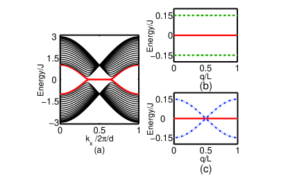
Figure 4: (color online) (a) Energy spectrum of a graphene strip (Möbius or generic), whose $(N,M)=(10,100)$, without external electric field. Obviously the edge states between the two Dirac points (red line) are approximately degenerate in the energy spectrum. A schematic illustration of the change in the energy spectrum is provided in (b) for a generic graphene strip and (c) for a Möbius graphene strip, which is caused by the applied uniform electric field on $y$ direction whose intensity $E$ satisfies $eEl(3N-1)/2=0.15J$. Here the red solid line represents the energy level of the edge states without the electric field, while the green dashed line and the blue dot-dashed line are the changed energy bands of the edge states in the electric field. Here, as the dual vector of $k_{x}$ in the inverse Fourier transformation applied only on the field operators of the edge states, $q$ is analogous to $x$.

In fact, the conducting behavior of the graphene strip (Möbius or generic) under perturbations (e.g., caused by a uniform electric field), is mainly determined by the properties of its edge states. For the generic graphene strip, a uniform electric field applied on $y$ direction will cause a perturbation Hamiltonian

$$H_{E}=-eE\sum_{i}y_{i}[\psi_{a}^{\dagger}(\mathbf{r_{i}})\psi_{a}(\mathbf{r_{i}})-\psi_{b}^{\dagger}(\mathbf{\widetilde{r_{i}}})\psi_{b}(\mathbf{\widetilde{r_{i}}})],$$ (19)

where $E$ is the electric field intensity. We assume here that the energy difference introduced by the electric field on opposite edges of the strip is much smaller than the hopping energy in graphene, namely, $3eENl\ll J$. Because the energy difference between edge states and bulk states with the same $k_{x}$ is much larger than the perturbation, transitions between them, induced by the electric field, can be neglected. Thus we only focus on transitions between different edge states in the following discussion.

Transition matrix elements between edge states are

$$\left\langle\Psi_{\pm}(k_{x})\right|H_{E}\left|\Psi_{\pm}(k_{x}^{\prime})\right\rangle= 0,$$ (20a)

$$\left\langle\Psi_{\pm}(k_{x})\right|H_{E}\left|\Psi_{\mp}(k_{x}^{\prime})\right\rangle= \epsilon_{k_{x}}\delta(k_{x},k_{x}^{\prime}),$$ (20b)

where $$\left|\Psi_{\pm}(k_{x})\right\rangle$$ are edge states for the generic graphene strip defined in Eq. (4), and

$$\epsilon_{k_{x}}=-eEl\left[1+\frac{3}{2}\left(N\frac{1+p_{k_{x}}^{4N}}{1-p_{k_{x}}^{4N}}-\frac{1}{1-p_{k_{x}}^{2}}\right)\right],$$ (20c)

with $$\delta(k_{x},k_{x}^{\prime})$$ the Kronecker delta function. Thus the modified energies of the edge states are

$$E_{e\pm}^{\prime}(k_{x})=\pm\sqrt{E_{e+}^{2}(k_{x})+\epsilon_{k_{x}}^{2}}.$$ (21)

When $N$ is sufficiently large,

$$\epsilon_{k_{x}}\simeq\epsilon_{\frac{\pi}{\sqrt{3}l}}=-\frac{1}{2}eEl(3N-1)$$

is approximately independent of momentum $k_{x}$. Equivalently, $\epsilon_{k_{x}}$ is approximately a constant in the range of $k_{x}$ where edge states exist. Besides, when the electric field is sufficiently strong but $E\ll J/3eNl$ still holds, the energy $E_{e\pm}(k_{x})$ of the original edge states approaches zero in comparison with $|\epsilon_{k_{x}}|$, namely, $|\epsilon_{k_{x}}|\gg E_{e+}(k_{x})$. In this sense, we approximately obtain

$$E_{e\pm}^{\prime}(k_{x})=\pm\epsilon_{\frac{\pi}{\sqrt{3}l}}.$$ (22)

The above argument means that the originally highly degenerate energy level of edge states ($E_{e\pm}(k_{x})\simeq 0$) is split into two separate energy levels by the uniform electric field (see Fig. 4(b)). This result could be simply interpreted by the different electric potential on the upper and lower edges. Since a gap exists between the two energy levels, the zigzag edges of the graphene strip are no longer conductive.

We notice that the above conclusion is only valid for the case with generic strips. For a Möbius graphene strip, due to its inherent twisted structure, the perturbation Hamiltonian introduced by the uniform electric field on $y$ direction reads as

$$H_{E}^{(M)} = -eE\sum_{i}y_{i}[\psi_{a}^{\dagger}(\mathbf{r_{i}})\psi_{a}(\mathbf{r_{i}})-\psi_{b}^{\dagger}(\mathbf{\widetilde{r_{i}}})\psi_{b}(\mathbf{\widetilde{r_{i}}})]\cos\left(\frac{\pi}{L}x_{i}\right)$$ (23)

$$= -\frac{eE}{2}\sum_{k_{x},m=0}^{2N-1}y_{m}^{(a)}\{[\psi_{\alpha}^{\dagger}(k_{x},y_{m}^{(a)})\psi_{\beta}(k_{x},-y_{m}^{(a)})+H.c.]+[\psi_{\alpha}^{\dagger}(k_{x}+\frac{2\pi}{L},y_{m}^{(a)})\psi_{\beta}(k_{x},-y_{m}^{(a)})+H.c.]\}.$$

Here we have assumed a uniform twist for the structure of the strip. It follows from Eq. (23) that the electric field couples the upper strip with the lower one, and induces transitions between states with different $k_{x}$, making $k_{x}$ no longer conserved. For the same reason for a generic graphene strip, we still neglect the transition between edge states and bulk states. As a consequence, we only need to focus on the subspace spanned by all the edge states

$$\left|\Psi_{\uparrow\left(\downarrow\right)}(k_{x})\right\rangle=D_{e\uparrow\left(\downarrow\right)}^{\dagger}(k_{x})\left|vac\right\rangle.$$ (24)

The transition matrix elements between edge states on the same pseudo strip vanish, i.e.,

$$\left\langle\Psi_{\uparrow\left(\downarrow\right)}(k_{x})\right|H_{E}^{(M)}\left|\Psi_{\uparrow\left(\downarrow\right)}(k_{x}^{\prime})\right\rangle=0,$$ (25a)

while the nonzero matrix elements

$$\left\langle\Psi_{\downarrow}(k_{x}^{\prime})\right|H_{E}^{(M)}\left|\Psi_{\uparrow}(k_{x})\right\rangle=\left\langle\Psi_{\uparrow}(k_{x})\right|H_{E}^{(M)}\left|\Psi_{\downarrow}(k_{x}^{\prime})\right\rangle=\epsilon_{k_{x}}^{(M)}[\delta(k_{x},k_{x}^{\prime})+\delta(k_{x}+\frac{2\pi}{L},k_{x}^{\prime})]$$ (25b)

describe transitions between edge states on the upper and lower pseudo strips. Here $$\epsilon_{k_{x}}^{(M)}=\epsilon_{k_{x}}/2 p_{k_{x}} p_{k_{x}+2\pi/L}$$, and we have neglected the difference between and . Still, we approximately obtain

$$\epsilon_{k_{x}}^{(M)}=\epsilon_{\frac{\pi}{\sqrt{3}l}}^{(M)}=-\frac{1}{4}eEl(3N-1).$$

Since $$L k_{x} k_{x} E_{e\uparrow/\downarrow}(k_{x})\simeq 0 k_{x}$$ is large, is approximately continuous, and a large number of that satisfy Möbius boundary condition exist between the two Dirac points. The conclusion that is still valid for the Möbius graphene strip when is not in the vicinity of either Dirac point. Thus, the energies of the edge states in the presence of the uniform electric field are

$$E_{q}^{\prime}=\pm 2\epsilon_{\frac{\pi}{\sqrt{3}l}}^{(M)}\cos\left(\frac{\pi}{L}q\right),$$ (26)

where $q$ is dual vector of $k_{x}$ in the inverse Fourier transformation. It could be concluded that the originally highly degenerate energy level $E_{e\uparrow/\downarrow}(k_{x})=0$ is broadened, by the uniform electric field, into an energy band with width $4\epsilon_{\pi/\sqrt{3}l}^{(M)}$ (shown in Fig. 4(c)). A straightforward explanation for the energy band broadening is that the electric potential on the edge of the Möbius strip varies along the $x$ direction.

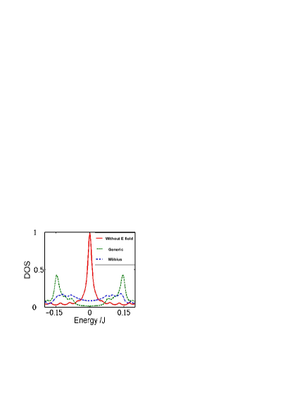
Figure 5: (color online) The density of state (DOS) near $\epsilon=0$ is obtained by deducing the retarded Green’s function $G(\epsilon)=(\epsilon-H+i\eta)^{-1}$ of the graphene strip with $\eta=0.01J$ and $(N,M)=(10,100)$, and determining the spectral function $A(\epsilon)=-2$Im$G(\epsilon)$. The black solid line, the green dashed line and the blue dash-dotted line represent the DOS of a graphene strip (Möbius or generic) without electric field, a generic graphene strip with uniform electric field, and a Möbius graphene strip with uniform electric field, respectively.

It is important to point out that there exist no energy gap for a Möbius graphene strip. The zigzag edge is still conductive even in presence of an external electric field. A Möbius graphene strip with such typical feature is referred to as a topological insulator. Numerical calculations for the density of states (DOS) near $\epsilon=0$ (Fig. 5) obviously support the above theoretical predictions. The DOS-energy curve explicitly demonstrates the existence of edge states in the vicinity of $\epsilon=0$ when no external electric field is applied. In this case, for both the generic and Möbius graphene strips, there is only one peak centered exactly at $\epsilon=0$, indicating high degeneracy of edge states. When uniform electric field is applied on a generic graphene strip, the peak turns to two peaks centered at $\pm\epsilon_{\pi/\sqrt{3}l}$, respectively, meaning that the highly degenerate energy level is split by the electric field. In this case, the DOS at $\epsilon=0$ approximately equals to zero, indicating the existence of a gap. Contrarily, with electric field applied on a Möbius graphene strip, the DOS has apparently nonzero value for any $\epsilon$ between $\pm\epsilon_{\pi/\sqrt{3}l}$. This numerical result agrees well with our above analytical prediction about the energy spectrum of generic and Möbius strips with and without external electric field, and indicates that the Möbius graphene strip is a topological insulator, but a generic strip is not.

IV NON-ABELIAN GAUGE FIELD AND OBSERVABLE EFFECTS IN TRANSMISSION

Figure 6: (color online) Schematic illustration of a Möbius graphene ring with two leads connected to its opposite sides and an external magnetic flux $\Phi_{I}$ thread its center.

In this section, we study the transportation properties of electrons in the Möbius graphene strip to demonstrate the topological effects similar to that for Möbius ladders Moladder1 . By comparing the Hamiltonian Eq. (15a) of a Möbius graphene strip with that of a generic graphene strip, it is recognized that, in the Möbius graphene strip, there is a phase shift on the hopping constant for the nearest neighbors $\left\langle i,j\right\rangle$ whose relative vectors $\mathbf{r_{i}}-\mathbf{r_{j}}$ have nonzero $x$ component. Similar to the case of the Möbius ladder, this phase shift in Eq. (16) can be described in terms of a non-Abelian gauge field

$$\mathbf{A}(\mathbf{r})=(A_{x},A_{y})=(\frac{c\hbar\pi}{eL},0)\theta(y)$$

in the continuous limit. The presence of this gauge field changes the canonical momentum $\mathbf{p}$ into $\mathbf{p}+e\mathbf{A}(\mathbf{r})$. The gauge field only exists in the lower strip, to result in an effective magnetic flux $\Phi=ch/2e$ along the positive $y$ direction thread the center of the lower strip, which is bent into a ring. Thus when an electron travels one round along the lower strip, such a gauge field may bring about a phase shift $\pi$. This effect could be experimentally testable when leads are connected on opposite sides of the strip (see Fig. 6). Then, there would be no transmission between two leads through the lower strip, due to the destructive interference between electrons passing through two possible paths from one lead to the other. Such destructive interference is analogous to that in the usual Aharonov-Bohm effect ABeffect1 ; ABeffect2 . However, this phenomenon in our system is totally induced by non-trivial topology, instead of a real magnetic flux.

To demonstrate the non-Abelian nature of the gauge field more clearly, we only consider the special graphene strip with only one regular hexagon along $y$ direction ($N=1$), which is simply an aromatic hydrocarbon chain (see Fig. 6). There are $4$ possible values of $y$ in the lattice of this strip, $y=\pm l/2$ and $y=\pm l$ respectively. The spinor representation of electrons in a regular hexagon lattice is

$$\Psi(x)=\left(\begin{array}[]{c}\psi_{a}(x)\\ \psi_{b}(x)\\ \psi_{a}^{\prime}(x)\\ \psi_{b}^{\prime}(x)\end{array}\right)\equiv\left(\begin{array}[]{c}\psi_{a}(x+\frac{\sqrt{3}}{2}l,l)\\ \psi_{b}(x,\frac{l}{2})\\ \psi_{a}(x,-\frac{l}{2})\\ \psi_{b}(x+\frac{\sqrt{3}}{2}l,-l)\end{array}\right),$$ (27)

where we have neglected differences in the $x$ coordinates between field operators and the $y$ coordinates have been omitted. Performing the unitary transformation $W$ on $\Psi(x)$ , we have

$$\widetilde{\Psi}(x)=W\Psi(x)=\frac{1}{\sqrt{2}}\left(\begin{array}[]{c}(\psi_{a}(x)-\psi_{b}^{\prime}(x))e^{i\frac{\pi}{L}x}\\ (\psi_{b}(x)-\psi_{a}^{\prime}(x))e^{i\frac{\pi}{L}x}\\ \psi_{a}^{\prime}(x)+\psi_{b}(x)\\ \psi_{b}^{\prime}(x)+\psi_{a}(x)\end{array}\right).$$ (28)

It can be verified that $\widetilde{\Psi}(x)$ is a periodic function since $\widetilde{\Psi}(x+L)=\widetilde{\Psi}(x)$. Then the Hamiltonian of the Möbius graphene strip becomes

$$H = -J\sum_{x}{\widetilde{\Psi}^{\dagger}(x)U\widetilde{\Psi}(x)+[\widetilde{\Psi}^{\dagger}(x)T\widetilde{\Psi}(x+\sqrt{3}l)+H.c.]}$$ (29)

$$= -J\sum_{k_{x}}\widetilde{\Psi}^{\dagger}(k_{x})[U+(Te^{i\sqrt{3}k_{x}l}+H.c.)]\widetilde{\Psi}(k_{x}),$$

where

$$U = \left(\begin{array}[]{cccc}0&1&0&0\\ 1&-1&0&0\\ 0&0&1&1\\ 0&0&1&0\end{array}\right),$$

$$T = \left(\begin{array}[]{cccc}0&e^{-i\frac{\pi}{M}}&0&0\\ 0&0&0&0\\ 0&0&0&0\\ 0&0&1&0\end{array}\right),$$

and

$$\widetilde{\Psi}(k_{x})=\frac{1}{\sqrt{M}}\sum_{x}\widetilde{\Psi}(x)e^{-ik_{x}x}.$$

In the continuous limit, the above Hamiltonian becomes

$$H=\int_{0}^{2\pi}d\varphi\widetilde{\Psi}^{\dagger}(\varphi)\{v[R(-i\frac{\partial}{\partial\varphi})-A_{0}]+R_{0}\}\widetilde{\Psi}(\varphi),$$ (32)

where $\varphi=2\pi x/L$, $v=2\pi\sqrt{3}lJ/L$, $R=$ diag$[-\sigma_{y},\sigma_{y}]$ ($\sigma_{y}$ is the Pauli matrix), $A_{0}=$diag$[\sigma_{y}/2,0]$, and $R_{0}=J$ diag$[0,1,-1,0]$. We would like to point out that in the continuous limit, we have expanded the original Hamiltonian in the $k_{x}$ representation around $k_{x}=\pi/\sqrt{3}l$. Because $A_{0}$ does not commute with $R_{0}$, $A_{0}$ is regarded as a non-Abelian gauge field. Actually, the observable effect of the non-Abelian gauge field can be explicitly demonstrated when the strip has small width, since in this case, a graphene strip may have distinct energy bands instead of strongly overlapped ones.

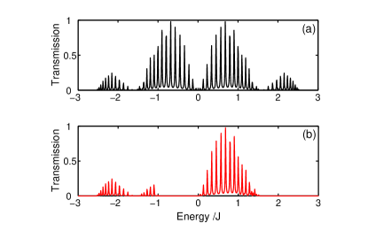
Figure 7: (color online) (a) and (b) show the transmission spectra of a generic graphene strip and a Möbius graphene strip, respectively, both of whose parameters $(N,M)=(1,40)$. Comparing (b) with (a), we find that several peaks in the transmission spectrum of the generic graphene strip are missing in that of the Möbius graphene strip, due to the existence of a non-Abelian gauge field in the latter one.

To obtain the transmission spectrum, we calculate the self energy Transport1

$$\Sigma_{L}(k^{\prime}_{x},k_{x})= -\frac{J^{\prime}}{2}e^{i\sqrt{3}k^{\prime}_{x}l}\left(\begin{array}[]{cccc}1&0&0&0\\ 0&0&0&0\\ 0&0&0&0\\ 0&0&0&1\end{array}\right),$$ (33e)

$$\Sigma_{R}(k^{\prime}_{x},k_{x})= -\frac{J^{\prime}}{2}e^{i(\sqrt{3}k^{\prime}_{x}l+\frac{1}{2}k_{x}L)}\left(\begin{array}[]{cccc}1&0&0&0\\ 0&0&0&0\\ 0&0&0&0\\ 0&0&0&1\end{array}\right)$$ (33j)

in the matrix representation (actually the whole matrix is a $4M\times 4M$ one made up of $M^{2}$ above $4\times 4$ blocks with respective $(k^{\prime}_{x},k_{x})$), and $J^{\prime}$ is the hopping energy in the leads ($J^{\prime}=1.5J$ in our numerical calculation). The above self energy results from the connection of two leads to the strip. Then we obtain the effective retarded Green function of the graphene strip

$$G(E(k))=\frac{1}{E(k)-H+i\eta-\Sigma_{L}-\Sigma_{R}},$$ (34)

where $E(k)=-2J^{\prime}\cos(\sqrt{3}kl)$ is the energy of electrons injected through the left lead, and $\eta=0_{+}$. After we determine the level broadening matrix $\Gamma_{L,R}=-2$Im$\Sigma_{L,R}$, the transmission coefficient

$$T(E(k))=\mathtt{Tr}[\Gamma_{R}G(E(k))\Gamma_{L}G^{{\dagger}}(E(k))]$$ (35)

is obtained in a straightforward way. The transmission spectrum of a generic graphene strip and a Möbius graphene strip (both width are $N=1$) are displayed in Fig. 7 (a) and (b), respectively. It is illustrated by Fig. 7(b) that incident electrons with energy $E\in[-J,0]$ are totally reflected by the Möbius graphene strip. This numerical result just confirm our heuristic prediction.

Since the non-Abelian gauge field exists in the lower strip instead of the upper one, there is a possible way to manipulate the transmission properties of the Möbius graphene strip through an external magnetic flux. As a magnetic flux $\Phi_{I}$ is applied thread the center of the Möbius strip (which has the shape of a ring), a magnetic vector potential appears on both the upper and lower pseudo strips. When the magnetic flux $\Phi_{I}$ is half of integer magnetic flux quanta, i.e., $\Phi_{I}=n\Phi_{0}/2$ with $\Phi_{0}=ch/e$ $(n=1,2,...)$, the total effective magnetic flux in the lower strip becomes $(n+1)\Phi_{0}/2$ and in the upper strip it becomes $n\Phi_{0}/2$. Consequently, when $n$ is even, quantum transmission is still suppressed in the lower strip, due to the destructive interference of electrons passing through two possible paths along the Möbius ring. Without such destructive interference, quantum transmission is allowed in the upper strip in this case. However, when $n$ is odd, quantum transmission is allowed in the lower strip and suppressed in the upper one. Based on the above discussion, changes in the positions of the peaks in the transmission spectrum are expected to be experimentally observed when the external magnetic flux changes. Numerical calculations, illustrated in Fig. 8, clearly verify our above heuristic discussions. Therefore, this magnetic-flux-based operation obviously implements quantum manipulation for electron transport in this Möbius nanostructure.

Figure 8: (color online) (a) and (b) show the transmission spectra of a Mö bius graphene ring, whose parameters $(N,M)=(1,40)$, with an external magnetic flux $\Phi_{I}=n\Phi_{0}/2$ thread its center, where $n$ is an integer. (a) corresponds to the $n=$even case, and (b) corresponds to the $n=$odd case, between which there are obvious differences in the position of the peaks in the transmission spectrum.

Next, we further consider the quantum transport of electrons in the low energy excitation regime. Actually, these electrons locate in the energy band of the edge states. The energies of edge states in both the lower and upper strips (see Fig. 3) are close to the Fermi level of the system. Here, the energies of the lower edge states are below the Fermi level, thus these edge states are all occupied at zero temperature. Contrarily, the upper edge states are not occupied at zero temperature, since their eigenenergies are above the Fermi level.

When there are an integer number of flux quanta thread the Möbius ring ($n$=even in the above discussion), or there exists no external magnetic flux thread the ring, the fact that quantum transmission is forbidden in the lower strip means that holes below the Fermi level cannot be current carriers. Then the only current carriers in the Möbius ring between two leads are electrons occupying the upper edge states (see Fig. 9(a)). Oppositely, when the number of flux quanta thread the ring is half-integer ($n$=odd in the above discussion), quantum transmission is forbidden in the upper strip. In this case, holes of the lower strip right below the Fermi level, instead of electrons occupying the upper edge states, become current carriers between the two leads (see Fig. 9(b)). Moreover, if the electron-electron and electron-phonon interactions could not be ignored in the Möbius graphene strip, the transmission rate of electrons and holes would be different significantly. Thus, accompanying the switch of current carriers between electrons and holes, transmission rate in the Möbius graphene strip may change as well.

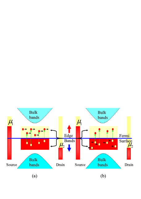
Figure 9: (color online) Schematic illustration of quantum transmission in a Möbius graphene ring with two leads connected to its opposite sides and an external magnetic flux $\Phi_{I}=n\Phi_{0}/2$ thread its center. Here, the up and down arrows represent the edge states in the upper and lower pseudo strips of the Möbius strip (see Fig. 3). (a) When $n=$even, the only current carriers are electrons occupying upper edge states above the Fermi level (red dots). (b) When $n=$odd, the only current carriers are holes in the energy band of lower edge states below the Fermi level (light yellow dots).

Finally, we remark on the effect of electric field on the transmission properties of the Möbius graphene strip. The uniform $y$ direction electric field applied to the Möbius graphene strip can induce strong coupling between electrons in the lower and upper strips. In this case, both of the strips can contribute significantly to quantum transmission. Therefore, the above forbidden transmission in one of the two pseudo strips no longer emerges in this case.

V CONCLUSION

Oriented by physical realizations of topological insulators and topological quantum devices, we theoretically studied the electronic properties of the Möbius graphene strip, which is an exotic 2D electron system with a topologically non-trivial edge. Various properties of the edge states were investigated through the tight binding model in this paper. We also studied the robustness of edge states in the Möbius graphene strip under perturbations, such as that caused by a uniform electric field. Analytical results about the exotic natures of such electron system are obtained for the first time and then confirmed by the following numerical calculations. Moreover, the physical effects of the non-Abelian induced gauge structure in the Möbius graphene strip were studied by considering the transmission spectrum of the Möbius graphene strip with two leads connected to its opposite sides. Based on such non-Abelian induced gauge field discovered, which is similar to that for the Möbius molecular devices studied in Ref. Moladder1 , we proposed a possible manipulation mechanism for the Möbius graphene strip through a magnetic flux. In fact, the robust edge of the Möbius graphene strip and the non-Abelian induced gauge field are two characteristic demonstrations of the nontrivial topology of the Möbius graphene strip. The above characters make the Möbius graphene strip as a candidate for topological insulators, which may benefit future applications in quantum coherent devices, and quantum information processing.

- (1) M. König, S. Wiedmann, C. Brüne, A. Roth, H. Buhmann, L. W. Molenkamp, X. L. Qi, and S. C. Zhang, Science 318, 766 (2008)
- (2) Y. Ran, Y. Zhang, and A. Vishwanath, Nature Phys. 5, 298 (2009).
- (3) S. C. Zhang, Physics. 1, 6 (2008).
- (4) J. E. Moore, Y. Ran, and X. G. Wen, Phys. Rev. Lett 101, 186805 (2008).
- (5) X. L. Qi, T. L. Hughes, and S. C. Zhang, Phys. Rev. B. 78, 195424 (2008).
- (6) J. Li, R. L. Chu, J. K. Jain, and S. Q. Shen, Phys. Rev. Lett. 102, 136806 (2009).
- (7) C. L. Kane and E. J. Mele, Phys. Rev. Lett. 95, 146802 (2005).
- (8) A. M. Essin, and J. E. Moore, Phys. Rev. B 76, 165307 (2007).
- (9) A. Bermudez, D. Patane, L. Amico, and M. A. Martin-Delgado, Phys. Rev. Lett. 102, 135702 (2009).
- (10) N. Zhao, H. Dong, S. Yang, and C. P. Sun, Phys. Rev. B 79, 125440 (2009).
- (11) D. Ajami, O. Oeckler, A. Simon, and R. Herges, Nature 426, 819 (2003).
- (12) S. Tanda, T. Tsuneta, Y. Okajima, K. Inagaki, K. Yamaya, and N. Hatakenaka, Nature 417, 397 (2002).
- (13) K. Wakabayashi, and K. Harigaya J. Phys. Soc. Jpn. 72, 998 (2003).
- (14) D. Jiang, and S. Dai J. Phys. Chem. C 112, 5348 (2008).
- (15) E. W. S. Caetano, V. N Freire, S. G. dos Santos, D. S. Galvão, and F. Sato, J. Chem. Phys. 128, 164719 (2008).
- (16) E. W. S. Caetano, V. N Freire, S. G. dos Santos, E. L. Albuquerque, D. S. Galvão, and F. Sato, Langmuir 25, 4751 (2009).
- (17) R. Saito, G. Dresselhaus, M. S. Dresselhaus, Physical Properties of Carbon Nanotubes (Imperial College Press, London, 1995).
- (18) M. S. Dresselhaus, G. Dresselhaus, P. Avouris, Carbon Nanotubes (Springer-Verlag, Berlin, 2000).
- (19) A. H. Castro, F. Guinea, N. M. R. Peres, K. S. Novoselov, and A. K. Geim, Rev. Mod. Phys. 81, 109 (2009).
- (20) K. Nakada, M. Fujita, G. Dresselhaus, and M. S. Dresselhaus, Phys. Rev. B 54, 17954 (1996).
- (21) K. Wakabayashi, M. Fujita, H. Ajiki, and M. Sigrist, Phys. Rev. B 59, 8271 (1999).
- (22) A. H. Castro Neto, F. Guinea, and N. M. R. Peres, Phys. Rev. B 73, 205408 (2006).
- (23) W. Yao, S. A. Yang, and Q. Niu, Phys. Rev. Lett. 102, 096801 (2009).
- (24) S. Datta, Quantum Transport, Atom to Transistor (Cambridge University Press, Cambridge, 2000).
- (25) Y. Aharonov, D. Bohm, Phys. Rev. 115, 485 (1959).
- (26) S. Nakamura, K. Wakabayashi, A. Yamashiro, and K. Harihaya, Physica E, 22, 684 (2004).