• montage: AGB nucleosynthesis with full $s$-process calculations

  R. P. Church^A,D, S. Cristallo^B, J. C. Lattanzio^A, R. J. Stancliffe^A, O. Straniero^B and R. C. Cannon^{C
  A} Centre for Stellar and Planetary Astrophysics, School of Mathematical Sciences, Monash University, Victoria 3800, Australia
  ^B INAF, Osservatorio Astronomico di Collurania, 64100 Teramo, Italy
  ^C Textensor Limited, 37 McDonald Road, Edinburgh, EH7 4LY, Scotland
  ^D Email: ross.church@sci.monash.edu.au

  Abstract:
  We present montage, a post-processing nucleosynthesis code that combines a traditional network for isotopes lighter than calcium with a rapid algorithm for calculating the $s$-process nucleosynthesis of the heavier isotopes. The separation of those parts of the network where only neutron-capture and beta-decay reactions are significant provides a substantial advantage in computational efficiency. We present the yields for a complete set of $s$-process isotopes for a $3\,\rm{M}_{\odot}$, $Z=0.02$ stellar model, as a demonstration of the utility of the approach. Future work will include a large grid of models suitable for use in calculations of Galactic chemical evolution.

  Keywords: nucleosynthesis — stars: AGB and post-AGB — stars: abundances — methods: numerical

1 Introduction

The asymptotic giant branch (AGB) is the final stage of the lives of low- and intermediate-mass stars. Evolution during the AGB phase is dominated by thermal pulses (Schwarzschild and Härm 1965). These cyclical events consist of brief, intense helium-burning pulses interspersed with quiescent hydrogen-burning interpulse phases. This complex behaviour produces significant nucleosynthesis. Of particular significance for the origin of the elements heavier than iron is the $s$-process. Neutrons produced by the ${}^{13}{\rm C}(\alpha,{\rm n})^{16}{\rm O}$ and ${}^{22}{\rm Ne}(\alpha,{\rm n})^{25}{\rm Mg}$ reactions are captured on to heavy metal isotopes, in particular ${}^{56}{\rm Fe}$. Through a sequence of neutron captures and beta decays this process can produce isotopes as heavy as lead and bismuth. The AGB and $s$-process nucleosynthesis are well covered in the literature; for example, see recent reviews of AGB evolution by Herwig (2005) and the $s$-process by Busso et al. (1999), as well as references therein and other contributions in this issue.

The recent history of $s$-process nucleosynthetic calculations is dominated by the work of Roberto Gallino and his collaborators, and is reviewed in detail elsewhere in this volume. Much of this work has been motivated by the abundant data provided in recent years by the analysis of meteoritic grains (Zinner 2008; Lugaro 2005) and by spectroscopic observations of giant stars (e.g. Lambert et al. 1995; Abia et al. 2002). Such calculations are challenging for several reasons. One problem is the large computational effort required. For stars that undergo thermal pulses the AGB is, by a large factor, the most difficult part of the evolutionary calculations. In order to reduce their run-time AGB structure calculations usually only include the reactions that generate substantial quantities of energy: the pp-chains, CNO cycles and helium-burning reactions. This allows a small nuclear network to be used. For nucleosynthetic calculations, however, a much larger network is required. To deal with this problem a post-processing technique is commonly employed, where the calculation of nuclear burning and mixing is decoupled from stellar structure and evolution calculations. The isotopes produced and destroyed via the $s$-process represent the majority of the nuclear network. One technique to deal with them is to assume an average neutron-absorption cross-section for the heavy isotopes and, by means of a fictitious particle, count the number of neutrons that they absorb (e.g. Busso et al. 1988). This then allows those neutrons to be distributed within the $s$-process network to calculate their nucleosynthetic effect. Alternatively a restricted s-process network can be used, containing a sub-section of the relevant isotopes (e.g. Karakas et al. 2008). A third approach has been followed by Straniero et al. (2006), who present an evolutionary model containing a full nuclear network coupled directly to their stellar evolution code (see also Cristallo et al. 2009).

We describe here a numerical technique that allows us to compute the nucleosynthesis of all the relevant isotopes at the same time with a reasonable computational effort. We split the nuclear network into two parts and solve them separately. The lower network comprises all elements up to and including potassium, and some calcium and scandium isotopes. The upper network contains all the heavier isotopes. The code for evaluating the lower network is briefly discussed in Section 2 and that for the upper network, along with the interface between the two, is described in Section 3. We describe a sample model and give its yields in Section 4.

2 monsoon and the lower network

To model the nucleosynthesis of species less massive than calcium we use monsoon, a post-processing nucleosynthesis code. It calculates the mixing and burning of a user-specified set of isotopes simultaneously using a standard relaxation method. As its input monsoon takes the radius, pressure, temperature, density, mixing length and velocity as a function of mass from separately calculated stellar structure models. We briefly cover the details of monsoon’s construction here; for more information the reader is referred to Cannon (1993), which describes an early version of the code, and Church et al. (in preparation).

monsoon comprises a one-dimensional, spherically-symmetric model. Material undergoing convection is split into two streams, one moving upwards and one downwards. In a given timestep material is mixed into each up-flowing cell from the cell below, and similarly into each down-moving cell from the cell above. A gradient in the vertical flow causes material to flow between the two cells in the same level. The ratio of the cross-sectional areas of the up-flowing and down-flowing streams can be adjusted. However, in the model computed here we assume that the two streams have the same cross-section.

We adopt a mesh composed of several sections, the number depending on the evolutionary phase. For main-sequence stars the mesh is placed at geometrically spaced intervals in mass, increasing from the core to envelope. When burning shells develop on the RGB and AGB they are treated with two additional sections of mesh each, also with geometrically-spaced — but closer — meshes. Cores and inter-shell regions are treated with meshes spaced at constant intervals in mass. As burning shells move out through the star the sections of mesh that represent them consume points from the region above and release points into the region below as necessary. Otherwise the mesh is held steady to reduce numerical diffusion. Some special treatment is needed to preserve sufficient resolution in the inter-shell region on the AGB and this is discussed in Section 3. It is important to note that the mesh that we adopt does not depend on that used for the structural input. This provides a substantial saving in computational effort; for example, the structure code must place many points in the outer envelope to deal with ionisation zones, whereas very little nucleosynthesis of any interest takes place in the envelope and hence very few points are required. Similarly we choose the timestep independently of that used to calculate the star’s structure.

Nuclear reactions are utilised in the parameterised reaclib form of Rauscher and Thielemann (2000). This utilises a seven-component fit to reaction rates that avoids the need for interpolation in large tables. Multiple fits may be made in the case of complex rates, in particular those exhibiting resonances. For the models presented in this paper we use the recommended rates of Illiadis (private communication).

To produce a ¹³C pocket and hence the required source of neutrons in low-mass stars we follow the prescription of (Karakas et al. 2008). For each thermal pulse where third dredge-up occurs a partially-mixed zone is artificially inserted at the bottom of the convective envelope at its point of maximum penetration into the star. Instead of trying to model the behaviour of the (unknown) process causing this partial mixing, we mimic its effect by modifying the hydrogen abundance to include an exponentially decaying profile just below the base of the convective zone. The capture of these protons by ¹²C naturally leads to a pocket of ¹³C forming, which burns via the ${}^{13}{\rm C}(\alpha,{\rm n})^{16}{\rm O}$ reaction to produce the dominant neutron source for the $s$-process in low-mass AGB stars. We find that for a star of this mass ($M\simeq 3\,\rm{M}_{\odot}$) a reasonable quantity of $s$-processing is obtained by choosing a zone of mass roughly one tenth that of the intershell region (Karakas et al. 2008).

3 Treatment of the $s$-process

To treat the $s$-process we use the network of Straniero et al. (2006) for isotopes from ⁴⁴Ca to ²⁰⁹Bi. In this part of the network the only reactions that we consider are neutron captures, beta decays and electron captures. In the conditions found in AGB stars proton- and alpha-capture reactions are not significant for these isotopes. Decays that occur rapidly are taken to be instantaneous. The network is terminated by the reactions

$${}^{210}{\rm Pb}({\rm n},\alpha\beta\beta)^{207}{\rm Pb}$$

$${}^{210}{\rm Bi}({\rm n},\alpha\beta)^{207}{\rm Pb}$$

$${}^{210}{\rm Po}({\rm n},\alpha)^{207}{\rm Pb}$$

and

$${}^{210}{\rm Po}(\alpha)^{206}{\rm Pb}.$$

The alpha particles produced by these reactions are not fed back into the lower network but are retained within the upper network and do not react. This is unlikely to lead to significant errors as the $s$-process occurs within helium-rich parts of the star where the contribution of the mechanism to the helium abundance is insignificant.

In order to increase the speed of the code such that it can produce useful results, the burning and mixing processes in the upper network are decoupled. A burning step takes place first, using the neutron abundances provided by the lower network, and the resulting isotopic abundances are then mixed. The mixing scheme used is, as in the lower network, that of Cannon (1993), and again the resulting equations are solved using a standard relaxation method. As a result of this simplification burning only needs to be calculated at a single meshpoint at a time, whereas mixing is only calculated for a single isotope at a time. This removes the need to invert very large matrices and hence makes the problem tractable. It may lead to some small loss of accuracy, but only for reactions that occur on a similar timescale to the mixing processes. Such reactions are, in these models, confined to the lower network, which is why simultaneous mixing and burning is employed there. The neutron capture reactions that dominate the upper network are in general much faster than convective mixing, whereas most of the $\beta$ decays are rather slower.

For reasons of simplicity the mesh and timestep used by the upper network are taken from the lower network. Occasionally the upper network may require a shorter timestep to converge: in these cases the step is broken into a set of several intervals of equal duration.

In order to resolve the ¹³C pocket and resulting $s$-process reactions well it is necessary to have good mass resolution in the intershell. We find that a good compromise between adequate resolution and code performance can be achieved by inserting a large number of points, of the order of 50, when the partially mixed zone is included at the point of maximum dredge-up. We then allow the code to add and remove points in the usual manner, provided that the removal of a point does not create a composition discontinuity greater than a factor of 1.3 between any of the lower-network abundances of the newly adjacent points. This is empirically found to retain sufficient resolution during the interpulse period as the pocket burns radiatively. At the peak of the next pulse the intershell convection zone reaches the remainder of the ¹³C pocket: the convective motions flatten the composition profile and hence the points are removed.

3.1 monsoon and the upper network

The interface between monsoon and the upper network is effected by means of the species ⁴⁴Ca and ⁴⁵Ca. These two isotopes are included in both networks. Their molar fractions, $h^{\prime}$, in the lower network are given, in terms of molar fractions $h$ of species in the upper network, by

$$h^{\prime}_{{}^{44}\rm Ca}=\sum h_{i}$$

$$h^{\prime}_{{}^{45}\rm Ca}\simeq 0$$

where the sum runs over all the species in the upper network. In the lower network there are two reactions that involve both species:

$${}^{44}{\rm Ca}({\rm n},\gamma)^{45}{\rm Ca}$$

and

$${}^{45}{\rm Ca}({\rm g})^{44}{\rm Ca}.$$

The fictitious particle g is included to count the number of neutron captures that the material in the upper network has undergone. The rate of the second reaction is chosen to be very fast, so that any neutron captured produces a g particle in effect instantaneously. This constrains the abundance of ${}^{45}{\rm Ca}$ in the lower network to be very close to zero at all times, although it could take a small but finite value in regions with a very large neutron exposure. The cross-section, $\sigma_{\rm{}^{44}Ca,n}$, of the first reaction is calculated as a weighted sum across all the n-capture reactions in the upper network:

$$\sigma_{\rm{}^{44}Ca,n}=\sum h_{i}\sigma_{i,{\rm n}}/h^{\prime}_{{}^{44}\rm Ca}$$ (1)

where the sum once again runs over all the species in the upper network. This allows the number of neutrons captured in the upper network to be calculated self-consistently, and subsequently used to calculate the changes in abundance in the upper network.

4 Model and yield

As a sample model we present a $3\,\rm{M}_{\odot}$, $Z=0.02$ star. The structure model sequence was computed using the Monash version of the Mount Stromlo Stellar Structure Programme (monstar, Lattanzio 1986; Frost and Lattanzio 1996). The opacities used by the code have been updated. At high temperatures we use the OPAL opacities (Iglesias and Rogers 1996), and at low temperatures the opacity tables from Ferguson et al. (2005). We use the Kudritzki and Reimers (1978) mass-loss law on the first giant branch and during core helium burning with $\eta=0.4$, and the AGB mass-loss law of Vassiliadis and Wood (1993) thereafter. Our initial abundances are taken from Anders and Grevesse (1989). The model was evolved from the pre-main sequence through to the late stages of the AGB where numerical instabilities prevented any further evolution. The helium-burning luminosity as a function of time during the AGB is shown in Figure 1. Dredge-up takes place during the last 35 thermal pulses: the very final pulse does not evolve as far as dredge-up and hence is not included. At the end of the calculation the model has lost a total of $1.77\,\rm{M}_{\odot}$ of material in winds and has a hydrogen-exhausted core mass of $0.71\,\rm{M}_{\odot}$, with $0.52\,\rm{M}_{\odot}$ remaining in the envelope. Given the mass-loss rate of $2.16\times 10^{-5}\,\rm{M}_{\odot}\,{\rm yr^{-1}}$ and interpulse period of $3.3\times 10^{4}\,{\rm yr}$ prevailing at the end of the simulation this suggests that there are two thermal pulses missing, including the final pulse that does not converge.

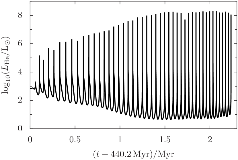
Figure 1: The helium burning luminosity of our $3\,\rm{M}_{\odot}$, $\rm{Z}_{\odot}$ star is shown as a function of time during the AGB. The time at the start of the plot is chosen to precede the onset of oscillations in the helium-burning luminosity. The sharp spikes are thermal pulses, a total of 45 of which can be seen.

We find that we have both a larger final core mass and more thermal pulses than the corresponding model of Karakas and Lattanzio (2007), which was calculated with a different version of the same code. This is because we have used updated physical data, including a larger mixing length parameter and updated low-temperature opacities. These changes lead to a later onset of the super-wind, hence a larger core and increased number of thermal pulses.

4.1 Nucleosynthesis during a sample pulse

For each pulse with dredge-up we add a partially-mixed zone as described in Section 2. This then goes on to form a ${}^{13}{\rm C}$ pocket through the capture of protons on to ${}^{12}{\rm C}$. As an example we present the evolution of the isotopic abundances during the twelfth thermal pulse. Following Karakas et al. (2008) we add a partially-mixed zone of mass $10^{-3}\,\rm{M}_{\odot}$ – chosen to be about one tenth of the total intershell mass – at the point of maximum dredge-up. Figure 2 shows the effect on the most structurally-important isotopes.

Panel (a) shows conditions $10^{3}\,{\rm years}$ after the maximum extent of dredge-up. The partially-mixed zone has been added and has partially burnt already to produce some ${}^{14}{\rm N}$ and ${}^{13}{\rm C}$. Panel (b) is part-way into the interpulse phase. The part of the partially mixed zone with the largest abundance of protons has burnt into CNO equilibrium, so the most abundant CNO isotope is ${}^{14}{\rm N}$. Further in to the star a larger quantity of ${}^{13}{\rm C}$ has been able to form. Panel (c) is from about 2/3 of the way through the interpulse period. The majority of the ${}^{13}{\rm C}$ formed has burnt to ${}^{16}{\rm O}$, via the neutron-producing alpha-capture reaction. The final panel, (d), shows the state of the intershell just before the 13th thermal pulse. The ${}^{13}{\rm C}$ has been almost completely burned.

Figure 3 shows the effect of the ${}^{13}{\rm C}$ pocket and subsequent neutron production on a selection of $s$-process isotopes. The discontinuity between the abundances in the envelope and those in the intershell is caused by previous $s$-process episodes, caused by the ${}^{13}{\rm C}$$(\alpha,{\rm n})$${}^{16}{\rm O}$ reaction during the interpulse periods and the ${}^{22}{\rm Ne}$$(\alpha,{\rm n})$${}^{25}{\rm Mg}$ reaction which is eventually activated at the pulse peaks. The chemical signatures of these previous thermal pulses remain within the intershell region and are mixed at each pulse peak by the partially-overlapping intershell convection zones. The isotopes shown were selected to show the effect of a moderate neutron exposure on isotopes with a range of different formation and destruction pathways and neutron-capture cross-sections. ${}^{56}{\rm Fe}$ is the initially most abundant $s$-process isotope and hence the only discernible effect on its abundance is destruction by absorption of neutrons. Similarly, ${}^{58}{\rm Ni}$ is synthesised in supernovae, not by the $s$-process: it is also only destroyed by neutron absorption. ${}^{59}{\rm Co}$ is both produced and destroyed at different mass co-ordinates in the star, depending on the degree of neutron absorption. Starting from the majority seed, ${}^{56}{\rm Fe}$, ${}^{59}{\rm Co}$ requires only three neutrons to be captured and hence is produced in the regions of the pocket with a lower neutron exposure. Towards the centre of the pocket where the neutron flux is higher it is on average depleted. The other two isotopes, ${}^{85}{\rm Rb}$ and ${}^{208}{\rm Pb}$, show only production, as they lie further up the $s$-process and hence require a large number of neutrons to be absorbed by a seed for their production.

4.2 Comparison with single-network approach

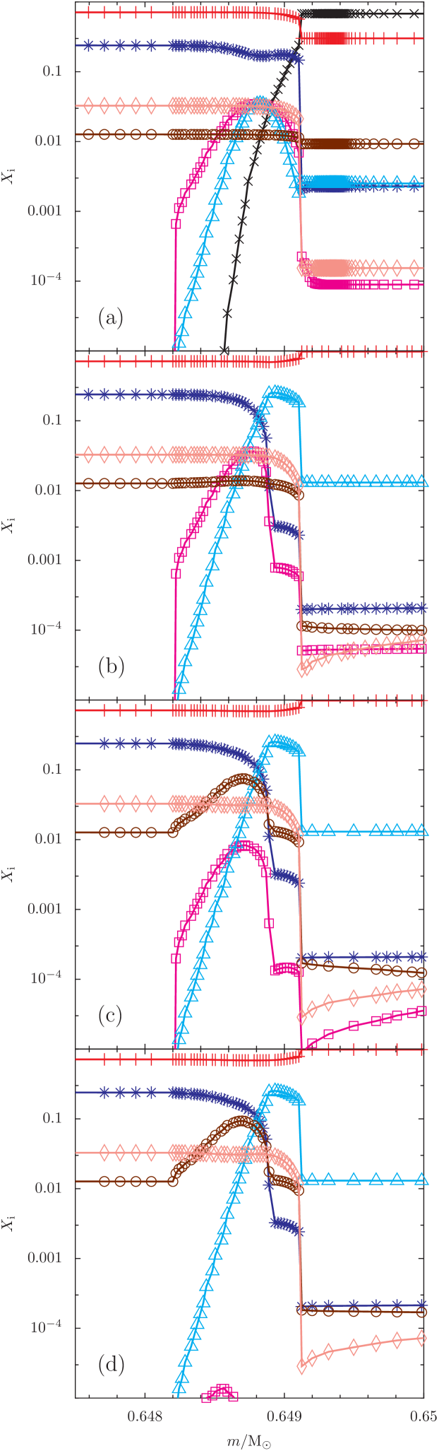
Figure 2: Isotopic abundances for structurally-significant isotopes at four points spanning the 12th thermal pulse and subsequent interpulse period. Black lines with crosses show hydrogen, red lines with plusses ${}^{4}{\rm He}$, blue lines with stars ${}^{12}{\rm C}$, magenta lines with squares ${}^{13}{\rm C}$, cyan lines with triangles ${}^{14}{\rm N}$, brown lines with circles ${}^{16}{\rm O}$ and pink lines with diamonds ${}^{22}{\rm Ne}$.

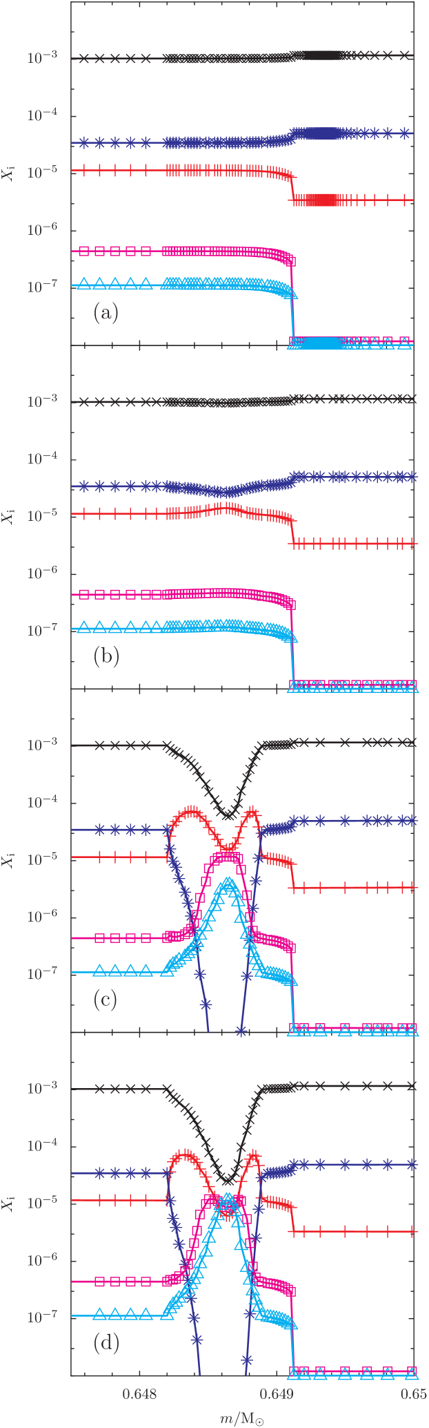
Figure 3: Isotopic abundances for selected $s$-process isotopes at the same times as the corresponding panels in Figure 2. Black lines with crosses show ${}^{56}{\rm Fe}$, red lines with plusses ${}^{59}{\rm Co}$, blue lines with stars ${}^{58}{\rm Ni}$, magenta lines with squares ${}^{85}{\rm Rb}$ and cyan lines with triangles ${}^{208}{\rm Pb}$.

As part of the testing process we created a version of monsoon with an extended network, that went as far as ${}^{98}{\rm Zr}$. This was used to model the first few thermal pulses of the model, as was a version of montage with a cut-down $s$-process network. The adopted truncation of the network reduces the runtime for the monsoon calculation to a manageable level, allowing us to compute the models presented here in under a week. The nuclear physics input data for the $s$-process network in montage was changed so that the same reaction rates were used as in monsoon. A selected set of intershell abundances from the end of the second thermal pulse in both codes are shown in Figure 4. It can be seen that, phenomenologically, the abundance profiles look very similar but that there are small differences between the abundances calculated, particularly at the point of highest neutron exposure. Closer investigation of the internals of the codes revealed that this was due to the different methods used to interpolate reaction rates in temperature: monsoon evaluates the rate for a given temperature from the reaclib formulae, whereas the $s$-process network in montage interpolates in $\log T$ within a pre-computed table. This leads to a systematically higher reaction rate in montage owing to the shape of the rate function at these temperatures. We found that the differences in abundances were consistent with these inconsistencies in reaction rates.

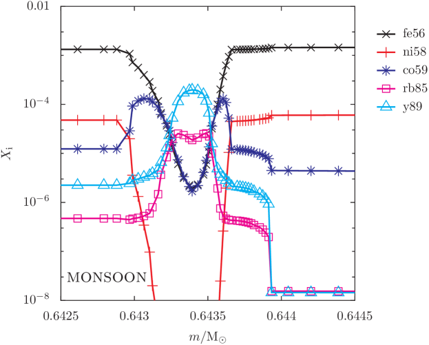
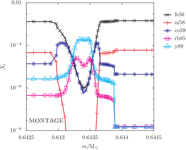
Figure 4: Isotopic abundances for selected $s$-process isotopes at the end of the second thermal pulse for the codes with a reduced $s$-process network. The top panel shows results for monsoon, the bottom panel those for montage. Black lines with crosses show ${}^{56}{\rm Fe}$, red lines with plusses ${}^{58}{\rm Ni}$, blue lines with stars ${}^{59}{\rm Co}$, magenta lines with squares ${}^{58}{\rm Rb}$ and cyan lines with triangles ${}^{89}{\rm Y}$.

4.3 Yields

Following Karakas and Lattanzio (2007) we provide yields for the isotopes that we include (Tables 4.3 and LABEL:tab:yields2). To save space we present only the initial (Solar) value of the mass fraction for each isotope, $X_{i}(0)$, and its average value in the ejecta, $\left<X_{i}\right>$. Our model still retained some envelope at the point where the evolution terminated, and the composition of this material is included when taking the average. Although we would expect two additional thermal pulses to take place whilst the remaining envelope was being lost they are unlikely to change the yield greatly as they will represent a small fraction of the total number of thermal pulses. A more sophisticated approach would be to synthesise two additional thermal pulses, as in Karakas and Lattanzio (2007).

The yield, commonly defined as

$$p_{i}=\int_{0}^{\tau}\left[X_{i}(t)-X_{i}(0)\right]\frac{\mathrm{d}M}{\mathrm{d}t}\mathrm{d}t,$$ (2)

can be found as $p_{i}=\left[\left<X_{i}\right>-X_{i}(0)\right]\Delta M$, where $\Delta M=2.29\,\rm{M}_{\odot}$ is the total mass lost by the star, including the envelope remaining at the end of the calculation.

Table 1: Yields from a $3\,\rm{M}_{\odot}$, $Z=0.02$ model (see text for details). Continued in Table 2.

Isotope $i$	$\left<X_{i}\right>$	$X_{i}(0)$	Isotope $i$	$\left<X_{i}\right>$	$X_{i}(0)$	Isotope $i$	$\left<X_{i}\right>$	$X_{i}(0)$
${\rm g}$ 1	$2.999$E$-04$	$2.977$E$-04$	${}^{55}{\rm Fe}$	$6.302$E$-07$	$0.000$E$+00$	${}^{94}{\rm Mo}$	$7.128$E$-10$	$5.829$E$-10$
${\rm p}$	$6.205$E$-01$	$6.879$E$-01$	${}^{56}{\rm Fe}$	$1.148$E$-03$	$1.167$E$-03$	${}^{95}{\rm Mo}$	$8.523$E$-09$	$1.014$E$-09$
${}^{3}{\rm He}$	$8.963$E$-05$	$8.544$E$-07$	${}^{57}{\rm Fe}$	$3.590$E$-05$	$2.848$E$-05$	${}^{96}{\rm Mo}$	$1.260$E$-08$	$1.073$E$-09$
${}^{4}{\rm He}$	$3.413$E$-01$	$2.931$E$-01$	${}^{58}{\rm Fe}$	$1.095$E$-05$	$3.688$E$-06$	${}^{97}{\rm Mo}$	$4.655$E$-09$	$6.210$E$-10$
${}^{7}{\rm Li}$	$7.237$E$-12$	$3.550$E$-20$	${}^{60}{\rm Fe}$	$1.090$E$-07$	$0.000$E$+00$	${}^{98}{\rm Mo}$	$1.629$E$-08$	$1.585$E$-09$
${}^{12}{\rm C}$	$1.743$E$-02$	$3.035$E$-03$	${}^{59}{\rm Co}$	$4.632$E$-06$	$3.444$E$-06$	${}^{100}{\rm Mo}$	$1.286$E$-09$	$6.456$E$-10$
${}^{13}{\rm C}$	$8.063$E$-05$	$3.654$E$-05$	${}^{60}{\rm Co}$	$6.540$E$-12$	$0.000$E$+00$	${}^{97}{\rm Tc}$	$9.579$E$-13$	$0.000$E$+00$
${}^{14}{\rm C}$	$3.640$E$-09$	$0.000$E$+00$	${}^{58}{\rm Ni}$	$4.858$E$-05$	$5.057$E$-05$	${}^{98}{\rm Tc}$	$1.053$E$-13$	$0.000$E$+00$
${}^{14}{\rm N}$	$2.286$E$-03$	$1.106$E$-03$	${}^{59}{\rm Ni}$	$6.309$E$-07$	$0.000$E$+00$	${}^{99}{\rm Tc}$	$2.032$E$-09$	$0.000$E$+00$
${}^{15}{\rm N}$	$2.053$E$-06$	$4.367$E$-06$	${}^{60}{\rm Ni}$	$2.092$E$-05$	$2.000$E$-05$	${}^{96}{\rm Ru}$	$2.376$E$-10$	$2.574$E$-10$
${}^{16}{\rm O}$	$8.960$E$-03$	$9.602$E$-03$	${}^{61}{\rm Ni}$	$1.493$E$-06$	$8.804$E$-07$	${}^{98}{\rm Ru}$	$8.579$E$-11$	$8.948$E$-11$
${}^{17}{\rm O}$	$1.906$E$-05$	$3.891$E$-06$	${}^{62}{\rm Ni}$	$3.731$E$-06$	$2.843$E$-06$	${}^{99}{\rm Ru}$	$6.965$E$-10$	$6.106$E$-10$
${}^{18}{\rm O}$	$1.520$E$-05$	$2.169$E$-05$	${}^{63}{\rm Ni}$	$9.193$E$-08$	$0.000$E$+00$	${}^{100}{\rm Ru}$	$7.636$E$-09$	$6.119$E$-10$
${}^{19}{\rm F}$	$5.940$E$-06$	$4.055$E$-07$	${}^{64}{\rm Ni}$	$1.662$E$-06$	$7.438$E$-07$	${}^{101}{\rm Ru}$	$2.346$E$-09$	$8.339$E$-10$
${}^{20}{\rm Ne}$	$1.648$E$-03$	$1.621$E$-03$	${}^{63}{\rm Cu}$	$9.166$E$-07$	$6.103$E$-07$	${}^{102}{\rm Ru}$	$9.467$E$-09$	$1.565$E$-09$
${}^{21}{\rm Ne}$	$5.878$E$-06$	$4.131$E$-06$	${}^{65}{\rm Cu}$	$6.137$E$-07$	$2.806$E$-07$	${}^{104}{\rm Ru}$	$1.672$E$-09$	$9.446$E$-10$
${}^{22}{\rm Ne}$	$3.954$E$-03$	$1.303$E$-04$	${}^{64}{\rm Zn}$	$1.154$E$-06$	$1.046$E$-06$	${}^{103}{\rm Rh}$	$2.630$E$-09$	$9.315$E$-10$
${}^{23}{\rm Na}$	$1.334$E$-04$	$3.342$E$-05$	${}^{66}{\rm Zn}$	$1.007$E$-06$	$6.186$E$-07$	${}^{104}{\rm Pd}$	$5.413$E$-09$	$4.211$E$-10$
${}^{24}{\rm Mg}$	$5.184$E$-04$	$5.153$E$-04$	${}^{67}{\rm Zn}$	$1.787$E$-07$	$9.229$E$-08$	${}^{105}{\rm Pd}$	$2.176$E$-09$	$8.522$E$-10$
${}^{25}{\rm Mg}$	$1.070$E$-04$	$6.773$E$-05$	${}^{68}{\rm Zn}$	$8.792$E$-07$	$4.283$E$-07$	${}^{106}{\rm Pd}$	$7.181$E$-09$	$1.053$E$-09$
${}^{26}{\rm Mg}$	$1.349$E$-04$	$7.768$E$-05$	${}^{70}{\rm Zn}$	$1.448$E$-08$	$1.458$E$-08$	${}^{107}{\rm Pd}$	$1.223$E$-09$	$0.000$E$+00$
${}^{27}{\rm Al}$	$6.327$E$-05$	$5.804$E$-05$	${}^{69}{\rm Ga}$	$1.118$E$-07$	$4.019$E$-08$	${}^{108}{\rm Pd}$	$8.646$E$-09$	$1.038$E$-09$
${}^{28}{\rm Si}$	$6.495$E$-04$	$6.537$E$-04$	${}^{71}{\rm Ga}$	$9.499$E$-08$	$2.744$E$-08$	${}^{110}{\rm Pd}$	$1.074$E$-09$	$4.515$E$-10$
${}^{29}{\rm Si}$	$3.690$E$-05$	$3.429$E$-05$	${}^{70}{\rm Ge}$	$1.676$E$-07$	$4.397$E$-08$	${}^{107}{\rm Ag}$	$6.344$E$-10$	$6.925$E$-10$
${}^{30}{\rm Si}$	$2.655$E$-05$	$2.354$E$-05$	${}^{72}{\rm Ge}$	$2.059$E$-07$	$6.045$E$-08$	${}^{109}{\rm Ag}$	$2.584$E$-09$	$6.554$E$-10$
${}^{31}{\rm P}$	$1.112$E$-05$	$8.163$E$-06$	${}^{73}{\rm Ge}$	$5.901$E$-08$	$1.745$E$-08$	${}^{108}{\rm Cd}$	$5.406$E$-11$	$3.974$E$-11$
${}^{32}{\rm S}$	$3.929$E$-04$	$3.962$E$-04$	${}^{74}{\rm Ge}$	$2.678$E$-07$	$8.276$E$-08$	${}^{110}{\rm Cd}$	$6.640$E$-09$	$5.680$E$-10$
${}^{33}{\rm S}$	$3.840$E$-06$	$3.225$E$-06$	${}^{76}{\rm Ge}$	$1.807$E$-08$	$1.816$E$-08$	${}^{111}{\rm Cd}$	$2.701$E$-09$	$5.874$E$-10$
${}^{34}{\rm S}$	$1.913$E$-05$	$1.868$E$-05$	${}^{75}{\rm As}$	$2.930$E$-08$	$1.263$E$-08$	${}^{112}{\rm Cd}$	$8.943$E$-09$	$1.117$E$-09$
${}^{36}{\rm S}$	$1.499$E$-07$	$9.389$E$-08$	${}^{76}{\rm Se}$	$7.521$E$-08$	$1.279$E$-08$	${}^{113}{\rm Cd}$	$2.829$E$-09$	$5.709$E$-10$
${}^{35}{\rm Cl}$	$2.501$E$-06$	$2.535$E$-06$	${}^{77}{\rm Se}$	$3.546$E$-08$	$1.094$E$-08$	${}^{114}{\rm Cd}$	$1.231$E$-08$	$1.354$E$-09$
${}^{36}{\rm Cl}$	$5.508$E$-09$	$0.000$E$+00$	${}^{78}{\rm Se}$	$1.268$E$-07$	$3.442$E$-08$	${}^{116}{\rm Cd}$	$1.461$E$-09$	$3.592$E$-10$
${}^{37}{\rm Cl}$	$1.792$E$-06$	$8.554$E$-07$	${}^{79}{\rm Se}$	$2.608$E$-08$	$0.000$E$+00$	${}^{113}{\rm In}$	$2.108$E$-11$	$2.306$E$-11$
${}^{36}{\rm Ar}$	$7.620$E$-05$	$7.748$E$-05$	${}^{80}{\rm Se}$	$2.554$E$-07$	$7.525$E$-08$	${}^{115}{\rm In}$	$2.788$E$-09$	$5.224$E$-10$
${}^{38}{\rm Ar}$	$1.580$E$-05$	$1.540$E$-05$	${}^{82}{\rm Se}$	$1.331$E$-08$	$1.342$E$-08$	${}^{114}{\rm Sn}$	$6.995$E$-11$	$7.450$E$-11$
${}^{39}{\rm Ar}$	$1.962$E$-10$	$0.000$E$+00$	${}^{79}{\rm Br}$	$1.790$E$-08$	$1.243$E$-08$	${}^{115}{\rm Sn}$	$3.643$E$-11$	$3.866$E$-11$
${}^{40}{\rm Ar}$	$6.522$E$-08$	$2.535$E$-08$	${}^{81}{\rm Br}$	$3.695$E$-08$	$1.239$E$-08$	${}^{116}{\rm Sn}$	$1.530$E$-08$	$1.672$E$-09$
${}^{39}{\rm K}$	$3.528$E$-06$	$3.473$E$-06$	${}^{80}{\rm Kr}$	$1.166$E$-08$	$2.605$E$-09$	${}^{117}{\rm Sn}$	$5.088$E$-09$	$8.902$E$-10$
${}^{40}{\rm K}$	$4.010$E$-08$	$5.242$E$-09$	${}^{81}{\rm Kr}$	$4.839$E$-09$	$0.000$E$+00$	${}^{118}{\rm Sn}$	$2.116$E$-08$	$2.834$E$-09$
${}^{41}{\rm K}$	$4.194$E$-07$	$2.634$E$-07$	${}^{82}{\rm Kr}$	$1.222$E$-07$	$1.377$E$-08$	${}^{119}{\rm Sn}$	$6.378$E$-09$	$1.013$E$-09$
${}^{40}{\rm Ca}$	$5.914$E$-05$	$5.996$E$-05$	${}^{83}{\rm Kr}$	$5.153$E$-08$	$1.396$E$-08$	${}^{120}{\rm Sn}$	$3.009$E$-08$	$3.879$E$-09$
${}^{41}{\rm Ca}$	$2.388$E$-08$	$0.000$E$+00$	${}^{84}{\rm Kr}$	$2.983$E$-07$	$7.035$E$-08$	${}^{122}{\rm Sn}$	$1.634$E$-09$	$5.604$E$-10$
${}^{42}{\rm Ca}$	$5.076$E$-07$	$4.200$E$-07$	${}^{85}{\rm Kr}$	$1.039$E$-10$	$0.000$E$+00$	${}^{124}{\rm Sn}$	$7.028$E$-10$	$7.117$E$-10$
${}^{43}{\rm Ca}$	$1.065$E$-07$	$8.982$E$-08$	${}^{86}{\rm Kr}$	$6.699$E$-08$	$2.197$E$-08$	${}^{121}{\rm Sb}$	$2.625$E$-09$	$5.343$E$-10$
${}^{44}{\rm Ca}$	$1.532$E$-06$	$1.476$E$-06$	${}^{85}{\rm Rb}$	$5.745$E$-08$	$1.133$E$-08$	${}^{123}{\rm Sb}$	$7.322$E$-10$	$4.038$E$-10$
${}^{46}{\rm Ca}$	$5.266$E$-09$	$2.959$E$-09$	${}^{87}{\rm Rb}$	$2.857$E$-08$	$4.471$E$-09$	${}^{122}{\rm Te}$	$3.312$E$-09$	$3.915$E$-10$
${}^{48}{\rm Ca}$	$1.439$E$-07$	$1.443$E$-07$	${}^{86}{\rm Sr}$	$9.243$E$-08$	$5.098$E$-09$	${}^{123}{\rm Te}$	$1.138$E$-09$	$1.367$E$-10$
${}^{45}{\rm Sc}$	$5.754$E$-08$	$4.069$E$-08$	${}^{87}{\rm Sr}$	$6.321$E$-08$	$3.605$E$-09$	${}^{124}{\rm Te}$	$6.625$E$-09$	$7.370$E$-10$
${}^{46}{\rm Ti}$	$2.492$E$-07$	$2.302$E$-07$	${}^{88}{\rm Sr}$	$9.072$E$-07$	$4.342$E$-08$	${}^{125}{\rm Te}$	$3.028$E$-09$	$1.108$E$-09$
${}^{47}{\rm Ti}$	$2.142$E$-07$	$2.146$E$-07$	${}^{90}{\rm Sr}$	$2.532$E$-10$	$0.000$E$+00$	${}^{126}{\rm Te}$	$1.373$E$-08$	$2.972$E$-09$
${}^{48}{\rm Ti}$	$2.156$E$-06$	$2.216$E$-06$	${}^{89}{\rm Y}$	$1.827$E$-07$	$1.086$E$-08$	${}^{128}{\rm Te}$	$6.148$E$-09$	$5.071$E$-09$
${}^{49}{\rm Ti}$	$2.356$E$-07$	$1.686$E$-07$	${}^{90}{\rm Y}$	$6.435$E$-14$	$0.000$E$+00$	${}^{130}{\rm Te}$	$5.387$E$-09$	$5.514$E$-09$
${}^{50}{\rm Ti}$	$2.625$E$-07$	$1.689$E$-07$	${}^{90}{\rm Zr}$	$1.589$E$-07$	$1.355$E$-08$	${}^{127}{\rm I}$	$4.176$E$-09$	$2.953$E$-09$
${}^{50}{\rm V}$	$8.952$E$-10$	$9.402$E$-10$	${}^{91}{\rm Zr}$	$4.272$E$-08$	$2.988$E$-09$	${}^{129}{\rm I}$	$2.874$E$-11$	$0.000$E$+00$
${}^{51}{\rm V}$	$3.845$E$-07$	$3.826$E$-07$	${}^{92}{\rm Zr}$	$6.210$E$-08$	$4.617$E$-09$	${}^{128}{\rm Xe}$	$3.588$E$-09$	$2.979$E$-10$
${}^{50}{\rm Cr}$	$7.274$E$-07$	$7.643$E$-07$	${}^{93}{\rm Zr}$	$1.867$E$-08$	$0.000$E$+00$	${}^{129}{\rm Xe}$	$4.828$E$-09$	$3.748$E$-09$
${}^{51}{\rm Cr}$	$6.988$E$-10$	$0.000$E$+00$	${}^{94}{\rm Zr}$	$6.944$E$-08$	$4.781$E$-09$	${}^{130}{\rm Xe}$	$7.566$E$-09$	$6.010$E$-10$
${}^{52}{\rm Cr}$	$1.514$E$-05$	$1.533$E$-05$	${}^{96}{\rm Zr}$	$4.960$E$-09$	$7.866$E$-10$	${}^{131}{\rm Xe}$	$5.410$E$-09$	$3.020$E$-09$
${}^{53}{\rm Cr}$	$1.753$E$-06$	$1.771$E$-06$	${}^{93}{\rm Nb}$	$1.618$E$-09$	$1.678$E$-09$	${}^{132}{\rm Xe}$	$1.622$E$-08$	$3.718$E$-09$
${}^{54}{\rm Cr}$	$6.234$E$-07$	$4.492$E$-07$	${}^{94}{\rm Nb}$	$3.326$E$-13$	$0.000$E$+00$	${}^{134}{\rm Xe}$	$2.066$E$-09$	$1.390$E$-09$
${}^{55}{\rm Mn}$	$1.324$E$-05$	$1.339$E$-05$	${}^{92}{\rm Mo}$	$8.647$E$-10$	$9.152$E$-10$	${}^{136}{\rm Xe}$	$1.146$E$-09$	$1.148$E$-09$
${}^{54}{\rm Fe}$	$6.855$E$-05$	$7.114$E$-05$	${}^{93}{\rm Mo}$	$5.236$E$-12$	$0.000$E$+00$

5 Discussion and future work

Our results demonstrate that we are able to efficiently calculate the nucleosynthesis of a large number of $s$-process isotopes, incorporating both the ${}^{13}{\rm C}$$(\alpha,{\rm n})$${}^{16}{\rm O}$ and ${}^{22}{\rm Ne}$$(\alpha,{\rm n})$${}^{25}{\rm Mg}$ neutron sources. The nucleosynthesis calculations presented here took approximately one CPU-week of time on a modern desktop computer. As can be seen in Figure 2 we considerably over-resolve the intershell region. The number of points here could most likely be reduced, which would lead to a substantial saving in runtime.

Our next target is to extend these results to a large grid of models. Ideally Galactic chemical evolution calculations need yields at masses separated by about $0.5\,\rm{M}_{\odot}$ at intermediate masses, possibly lower at the lowest masses, and much closer metallicity intervals than those currently available (Izzard, private communication). This will provide a standard, consistent set of yields for use in calculation of Galactic chemical evolution.

monsoon has hitherto always been used with the monstar stellar evolution code. During testing we attempted to use the evolution code of Stancliffe and Jeffery (2007) to provide output to drive montage. This worked very well; a simple approach of writing out every tenth evolution model to the nucleosynthesis code input file provided a frequency of data that converged well. Within the uncertainties provided by differences in reaction rates between the two codes, the light element abundances predicted by the two codes agreed well. We conclude that montage is a general post-processing nucleosynthesis code, which with a small amount of effort we should be able to use with any stellar evolution code, suitably modified to print out the relevant models. This will allow us, for example, to quantify the uncertainties in nucleosynthesis predictions caused by different evolutionary codes in a self-consistent manner.

6 Summary

The use of a separate network and subtly different computational technique for the main nucleosynthesis and $s$-process of a thermally-pulsing AGB star has a substantial advantage in terms of the computational effort required. We have calculated the full $s$-process yields of a $3\,\rm{M}_{\odot}$ star at Solar metallicity, as a demonstration of the utility of the approach. We intend to extend this work to a large grid of simulations suitable for inclusion in Galactic chemical evolution models, as well as by making the code available as a general post-processing tool.

Acknowledgements

We are very grateful to Simon Campbell for the use of his version of monstar. We would also like to thank our colleagues for useful discussions, in particular Amanda Karakas, Maria Lugaro and Carolyn Doherty. RJS and RPC are funded by the Australian Research Council’s Discovery Projects scheme under grants DP0879472 and DP0663447 respectively. SC and OS are supported by the Italian MIUR-PRIN 2006 Project ‘Final Phases of Stellar Evolution, Nucleosynthesis in Supernovae, AGB stars, Planetary Nebulae’.

References

- Abia et al. (2002) Abia, C., Domínguez, I., Gallino, R., Busso, M., Masera, S., Straniero, O., de Laverny, P., Plez, B., and Isern, J.: 2002, Ap.J. 579, 817
- Anders and Grevesse (1989) Anders, E. and Grevesse, N.: 1989, Geochimica et Cosmochimica Acta 53, 197
- Busso et al. (1999) Busso, M., Gallino, R., and Wasserburg, G. J.: 1999, ARA&A 37, 239
- Busso et al. (1988) Busso, M., Picchio, G., Gallino, R., and Chieffi, A.: 1988, Ap.J. 326, 196
- Cannon (1993) Cannon, R. C.: 1993, MNRAS 263, 817
- Cristallo et al. (2009) Cristallo, S., Straniero, O., Gallino, R., Piersanti, L., Domínguez, I., and Lederer, M. T.: 2009, Ap.J. 696, 797
- Ferguson et al. (2005) Ferguson, J. W., Alexander, D. R., Allard, F., Barman, T., Bodnarik, J. G., Hauschildt, P. H., Heffner-Wong, A., and Tamanai, A.: 2005, Ap.J. 623, 585
- Frost and Lattanzio (1996) Frost, C. A. and Lattanzio, J. C.: 1996, Ap.J. 473, 383
- Herwig (2005) Herwig, F.: 2005, ARA&A 43, 435
- Iglesias and Rogers (1996) Iglesias, C. A. and Rogers, F. J.: 1996, Ap.J. 464, 943
- Karakas and Lattanzio (2007) Karakas, A. and Lattanzio, J. C.: 2007, Publications of the Astronomical Society of Australia 24, 103
- Karakas et al. (2008) Karakas, A. I., van Raai, M. A., Lugaro, M., Sterling, N. C., and Dinerstein, H. L.: 2008, ArXiv e-prints
- Kudritzki and Reimers (1978) Kudritzki, R. P. and Reimers, D.: 1978, AAP 70, 227
- Lambert et al. (1995) Lambert, D. L., Smith, V. V., Busso, M., Gallino, R., and Straniero, O.: 1995, Ap.J. 450, 302
- Lattanzio (1986) Lattanzio, J. C.: 1986, Ap.J. 311, 708
- Lugaro (2005) Lugaro, M.: 2005, Stardust from meteorites. An introduction to presolar grains, Stardust from meteorites / Maria Lugaro. World Scientific Series in Astronomy and Astrophysics, Vol. 9, New Jersey, London, Singapore: World Scientific. ISBN 981-256-099-8, 2005, XIV, 209 pp.
- Rauscher and Thielemann (2000) Rauscher, T. and Thielemann, F.-K.: 2000, Atomic Data and Nuclear Data Tables 75, 1
- Schwarzschild and Härm (1965) Schwarzschild, M. and Härm, R.: 1965, Ap.J. 142, 855
- Stancliffe and Jeffery (2007) Stancliffe, R. J. and Jeffery, C. S.: 2007, MNRAS 375, 1280
- Straniero et al. (2006) Straniero, O., Gallino, R., and Cristallo, S.: 2006, Nuclear Physics A 777, 311
- Vassiliadis and Wood (1993) Vassiliadis, E. and Wood, P. R.: 1993, Ap.J. 413, 641
- Zinner (2008) Zinner, E.: 2008, Publications of the Astronomical Society of Australia 25, 7