On the Statistics of Cognitive Radio Capacity in Shadowing and Fast Fading Environments

Abstract

In this paper we consider the capacity of the cognitive radio (CR) channel in different fading environments under a “low interference regime”. First we derive the probability that the “low interference regime” holds under shadow fading as well as Rayleigh and Rician fast fading conditions. We demonstrate that this is the dominant case, especially in practical CR deployment scenarios. The capacity of the CR channel depends critically on a power loss parameter, $\alpha$, which governs how much transmit power the CR dedicates to relaying the primary message. We derive a simple, accurate approximation to $\alpha$ in Rayleigh and Rician fading environments which gives considerable insight into system capacity. We also investigate the effects of system parameters and propagation environment on $\alpha$ and the CR capacity. In all cases, the use of the approximation is shown to be extremely accurate.

I Introduction

Until recently, the frequency bands below $3.5$ GHz were thought to be severely congested. Due to the superior propagation conditions in the lower frequencies there is a desire for all services to find a place in this sought after “real estate”. However, spectrum occupancy measurements performed in the United States [1] show that spectrum scarcity cannot be confirmed by the measurements. Instead, the apparent congestion is due to the way in which spectrum is allocated into specific bands for specific services (i.e., fixed, mobile and broadcasting) and then by the national regulatory authorities who license the band/service combinations to private owners. Therefore even when the licensed owner is not using their spectrum, there is no access to other users, hence the apparent congestion. In order to improve spectrum occupancy and utilization, various regulatory bodies worldwide are considering the benefits offered by cognitive radio (CR) [2]. The key idea behind the deployment of CR is that greater utilization of spectrum can be achieved if they are allowed to co-exist with the incumbent licensed primary users (PUs) provided that they cause minimal interference. The CRs must therefore learn from the radio environment and adapt their parameters so that they can co-exist with the primary systems. The CR field has proven to be a rich source of challenging problems. A large number of papers have appeared on various aspects of CR, namely spectrum sensing (see [3, 4] and the references therein), fundamental limits of spectrum sharing [5], information theoretic capacity limits [6, 7, 8, 9, 10] etc.

The 2 user cognitive channel [6, 7, 8, 9, 10] consists of a primary and a secondary user. It is very closely related to the classic 2 user interference channel, see [11] and references therein. The formulation of the CR channel is due to Devroye et al. [6]. In this channel, the CR has a non-causal knowledge of the intended message of the primary and by employing dirty paper coding [12] at the CR transmitter it is able to circumvent the primary user’s interference to its receiver. However, the interference from the CR to the primary receiver remains and has the potential to cause a rate loss to the primary.

In recent work, Jovicic and Viswanath [8] have studied the fundamental limits of the capacity of the CR channel. They show that if the CR is able to devote a part of its power to relaying the primary message, it is possible to compensate for the rate loss to the primary via this additional relay. They have provided exact expressions for the PU and CR capacity of a 2 user CR channel when the CR transmitter sustains a power loss by devoting a fraction, $\alpha$, of its transmit power to relay the PU message. Furthermore, they have provided an exact expression for $\alpha$ such that the PU rate remains the same as if there was no CR interference. It should be stressed here that their system model is such that at the expense of CR transmit power, the PU device is always able to maintain a constant data rate. Hence, we focus on CR rate, $\alpha$ and their statistics. They also assume that the PU receiver uses a single user decoder. Their result holds for the so called low interference regime when the interference-to-noise ratio (INR) at the PU receiver is less than the signal-to-noise ratio (SNR) at the CR receiver. The authors in [10] also arrived at the same results in their parallel but independent work.

The Jovicic and Viswanath study is for a static channel, i.e., the direct and cross link gains are constants. In a system study, these gains will be random and subject to distance dependent path loss and shadow fading. Furthermore, the channel gains also experience fast fading. As the channel gains are random variables, the power loss parameter, $\alpha$, is also random.

In this paper we focus on the power loss, $\alpha$, the capacity of the CR channel and the probability that the “low interference regime” holds. The motivation for this work arises from the fact that maximum rate schemes for the CR in the low interference regime [8, 10] and the achievable rate schemes for the high interference regime [7, 9] are very different. Hence, it is of interest to identify which scenario is the most important. To attack this question we propose a simple, physically based geometric model for the CR, PU layout and compute the probability of the low interference regime. Results are obviously limited to this particular model but provide some insight into reasonable deployment scenarios. Since the results show the low interference regime can be dominant, it is also of interest to characterize CR performance via the $\alpha$ parameter. In this area we make the following contributions:

• Assuming lognormal shadowing, Rayleigh fading and path loss effects we derive the probability that the “low interference regime” holds. We also extend the results to Rician fading channels.

• In both Rayleigh and Rician fading environments we derive an approximation for $\alpha$ and its statistics. This extremely accurate approximation leads to simple interpretations of the effect of system parameters on the capacity.

• Using the statistics of $\alpha$ we investigate the mean rate loss of the CR and the cumulative distribution function (CDF) of the CR rates. For both the above we show their dependence on the propagation parameters.

• We also show how the mean value of $\alpha$ varies with the CR transmit power and therefore the CR coverage area.

This paper is organized as follows: Section II describes the system model. Section III derives the probability that the “low interference regime” holds and in Section IV an approximation for $\alpha$ is developed. Section V presents analytical and simulation results and some conclusions are given in Section VI.

II System Model

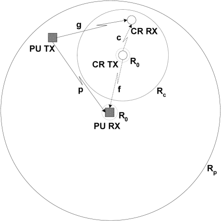
Figure 1: System model.

Consider a PU receiver in the center of a circular region of radius $R_{p}$. The PU transmitter is located uniformly in an annulus of outer radius $R_{p}$ and inner radius $R_{0}$ centered on the PU receiver. It is to be noted that we place the PU receiver at the center only for the sake of mathematical convenience (see Fig. 1). The use of the annulus restricts the length of the PU link from becoming too small. This matches physical reality and also avoids problems with the classical inverse power law relationship between signal strength and distance [13]. In particular, having a minimum distance, $R_{0}$, prevents the signal strength from becoming infinite as the transmitter approaches the receiver. Similarly, we assume that a CR transmitter is uniformly located in the same annulus. Finally, a CR receiver is uniformly located in an annulus centered on the CR transmitter. The dimensions of this annulus are defined by an inner radius, $R_{0}$, and an outer radius, $R_{c}$. This choice of system layout is asymmetric in the sense that the PU receiver is at the center of its circular region whereas the CR transmitter is at the center of its smaller region. This layout is chosen for mathematical simplicity since the lengths of the CR-PU and CR-CR links have a common simple distribution which leads to the closed form analysis in Sec. III. Following the work of Jovicic and Viswanath [8], the four channel gains which define the system are denoted $p,g,f,c$. In this paper, these complex channel gains include shadow fading, path-loss and Rayleigh and Rician fast fading effects. To introduce the required notation we consider the link from the CR transmitter to the PU receiver, the CP link. For this link we have:

$$|f|^{2}=\Gamma_{cp}|\tilde{f}|^{2},$$ (1)

where $|\tilde{f}|^{2}$ is an exponential random variable with unit mean for Rayleigh channels or a noncentral $\chi^{2}$ variable for Rician fading and $\Gamma_{cp}$ is the link gain. The link gain comprises shadow fading and distance dependent path loss effects so that,

$$\Gamma_{cp}=A_{c}L_{cp}r_{cp}^{-\gamma},$$ (2)

where $A_{c}$ is a constant that depends on physical deployment parameters such as antenna height, antenna gain, cable loss etc. In (2) the variable $L_{cp}=10^{\tilde{X}_{cp}/10}$ is lognormal, $\tilde{X}_{cp}$ is zero mean Gaussian and $r_{cp}$ is the link distance. The standard deviation which defines the lognormal is $\sigma$ (dB) and $\gamma$ is the path loss exponent. For convenience, we also write $L_{cp}=e^{X_{cp}}$ so that $X_{cp}=\beta\tilde{X}_{cp}$, $\beta=\ln(10)/10$ and $\sigma_{sf}^{2}$ is the variance of $X_{cp}$. Hence, for the CP link we have:

$$|f|^{2}=A_{c}e^{X_{cp}}r_{cp}^{-\gamma}|\tilde{f}|^{2}.$$ (3)

The other three links are defined similarly where $\tilde{p},\tilde{g},\tilde{c}$ are standard exponentials for Rayleigh fading and represent noncentral $\chi^{2}$ random variables for Rician fading, $X_{pp},X_{pc},X_{cc},$ are Gaussians with the same parameters as $X_{cp}$ and $r_{pp},r_{pc},r_{cc}$ are link distances. However, for the links involving the PU transmitter we assume a different constant $A_{p}$ in the model of link gains. The parameters $A_{p}$ and $A_{c}$ are constants and all links are assumed independent. The remaining parameters required are the transmit powers of the PU and CR devices, given by $P_{p}$ and $P_{c}$ respectively, and the noise powers at the PU and CR receivers, given by $N_{p}$ and $N_{c}$ respectively.

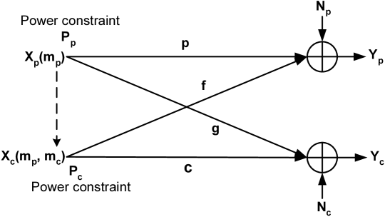
Figure 2: Information theoretic model (taken from [8]).

The physical model described above corresponds to the information theoretic model shown in Fig. 2. For fixed channel coefficients, $p,g,f$ and $c$, Jovicic and Viswanath [8] compute the highest rate that the CR can achieve subject to certain constraints using the model in Fig. 2. In this figure the arrow on the transmitter side indicates the noncausal availability of the PU’s message to the cognitive device for dirty paper coding (DPC) purposes [12]. A key constraint is that the PU must not suffer any rate degradation due to the CR and this is achieved by the CR dedicating a portion, $\alpha$, of its transmit power to relaying the PU message. The parameter, $\alpha$, is therefore central to determining the CR rate. Furthermore, the results in [8] are valid in the “low interference regime” defined by $a<1$ where:

$$a=\frac{\sqrt{N_{c}}\sqrt{\Gamma_{cp}}|\tilde{f}|}{\sqrt{N_{p}}\sqrt{\Gamma_{cc}}|\tilde{c}|}=\frac{\sqrt{N_{c}}e^{X_{cp}/2}r_{cp}^{-\gamma/2}|\tilde{f}|}{\sqrt{N_{p}}e^{X_{cc}/2}r_{cc}^{-\gamma/2}|\tilde{c}|}.$$ (4)

In this regime, the highest CR rate is given by

$$R_{CR}=\log_{2}\Bigg{(}1+\frac{|c|^{2}(1-\alpha)P_{c}}{N_{c}}\Bigg{)},$$ (5)

with the power loss parameter, $\alpha$, defined by

$$\alpha=\frac{|s|^{2}}{|t|^{2}}\Bigg{[}\frac{\sqrt{1+|t|^{2}(1+|s|^{2})}-1}{1+|s|^{2}}\Bigg{]}^{2},$$ (6)

where $|s|=\sqrt{P_{p}}\sqrt{\Gamma_{pp}}|\tilde{p}|N_{p}^{-1/2}$ and $|t|=\sqrt{P_{c}}\sqrt{\Gamma_{cp}}|\tilde{f}|N_{p}^{-1/2}$. Note that the definitions of $\alpha$ and $R_{c}$ are conditional on $a<1$. Since $a$ is a function of $\tilde{f}$ and $\tilde{c}$ we see that both $\tilde{f}$ and $\tilde{c}$ are conditional random variables.

III The low interference regime

Note that the $4$ paths which characterize the channels in Figs. 1 and 2 can all be Rayleigh or Rician. This leads to $16$ possible combinations of Rayleigh or Rician channels. To make the study more concise we assume that the PP and PC paths are Rayleigh and vary the CC and CP paths. Hence, we consider the $4$ combinations where $\tilde{c}$ (CC) and $\tilde{f}$ (CP) can be Rician or Rayleigh. This is sensible since $\tilde{c}$, $\tilde{f}$ affect both the low interference regime (4) and the cognitive rate ($R_{CR}$ in (5)), whereas the PP, PC links only affect $R_{CR}$. The notation Ray/Rice etc. denotes the nature of the $\tilde{f}/\tilde{c}$ variables or the CP/CC paths.

III-A Rayleigh/Rayleigh Scenario

The low interference regime is defined by $a<1$, where $a$ is defined in (4). The probability, $P(a<1)$, depends on the distribution of $r_{cc}/r_{cp}$. Using standard transformation theory [14], some simple but lengthy calculations show that the CDF of $r_{cc}/r_{cp}$ is given by (7). A sketch proof is given in Appendix I.

$$P\bigg{(}\frac{r_{cc}}{r_{cp}}<x\bigg{)}=\left\{\begin{array}[]{ll}0&\textrm{$x\leq\frac{R_{0}}{R_{p}}$}\\ \\ \frac{0.5x^{2}(R_{p}^{2}-R_{0}^{4}x^{-4})-R_{0}^{2}(R_{p}^{2}-R_{0}^{2}x^{-2})}{(R_{c}^{2}-R_{0}^{2})(R_{p}^{2}-R_{0}^{2})}&\textrm{$\frac{R_{0}}{R_{p}}<x\leq\frac{R_{c}}{R_{p}}$}\\ \\ \frac{0.5(R_{c}^{4}-R_{0}^{4})-R_{0}^{2}(R_{c}^{2}-R_{0}^{2})+(x^{2}R_{p}^{2}-R_{c}^{2})(R_{c}^{2}-R_{0}^{2})}{x^{2}(R_{c}^{2}-R_{0}^{2})(R_{p}^{2}-R_{0}^{2})}&\textrm{$\frac{R_{c}}{R_{p}}<x\leq 1$}\\ \\ 1-\frac{0.5R_{c}^{4}x^{2}+0.5R_{0}^{4}x^{2}-R_{0}^{2}R_{c}^{2}}{(R_{c}^{2}-R_{0}^{2})(R_{p}^{2}-R_{0}^{2})}&\textrm{$1<x\leq\frac{R_{c}}{R_{0}}$}\\ \\ 1&\textrm{$x>\frac{R_{c}}{R_{0}}$}\end{array}\right.$$ (7)

The CDF in (7) can be written as:

$$P\bigg{(}\frac{r_{cc}}{r_{cp}}<x\bigg{)}=c_{i0}x^{-2}+c_{i1}+c_{i2}x^{2}\quad\textrm{$i=1,2,3,4,5$}$$ (8)

where $\Delta=(R_{c}^{2}-R_{0}^{2})(R_{p}^{2}-R_{0}^{2})$, $c_{10}=0$, $c_{11}=0$, $c_{12}=0$, $c_{20}=0.5R_{0}^{4}/\Delta$, $c_{21}=-R_{0}^{2}R_{p}^{2}/\Delta$, $c_{22}=0.5R_{p}^{4}/\Delta$, $c_{30}=0.5(R_{0}^{4}-R_{c}^{4})/\Delta$, $c_{31}=R_{p}^{2}(R_{c}^{2}-R_{0}^{2})/\Delta$, $c_{32}=0$, $c_{40}=-0.5R_{c}^{4}/\Delta$, $c_{41}=1+R_{0}^{2}R_{c}^{2}/\Delta$, $c_{42}=-0.5R_{0}^{4}/\Delta$, $c_{50}=0$, $c_{51}=1$ and $c_{52}=0$.

Now $P(a<1)=P(a^{2}<1)$ can be written as $P(Y<Ke^{X}Z^{-\gamma})$ where $Y={|\tilde{f}|^{2}}/{|\tilde{c}|^{2}}$, $K=N_{p}/N_{c}$, $X=X_{cc}-X_{cp}$ and $Z=r_{cc}/r_{cp}$. Thus the required probability is:

$$P(Y<Ke^{X}Z^{-\gamma}) {}={} P(Z<K^{1/\gamma}e^{X/\gamma}Y^{-1/\gamma})$$ (9)

$${}={} E[P(Z<K^{1/\gamma}e^{X/\gamma}Y^{-1/\gamma}|X,Y)]$$

$${}={} E[P(Z<W|W)]$$

$${}={} \int_{0}^{\infty}P(Z<w)f_{W}(w)dw,$$

where $W=K^{1/\gamma}e^{X/\gamma}Y^{-1/\gamma}$ and $f_{W}(.)$ is the PDF of $W$. Note that $P(Z<w)$, given in (8), only contains constants and terms involving $w^{\pm 2}$. Hence, we need the following:

$$\int_{\theta}^{\kappa}\!\!w^{2m}f_{W}(w)dw=\int\!\!\int\!(Ke^{x}y^{-1})^{2m/\gamma}f_{X,Y}(x,y)dxdy,$$ (10)

where $m=-1,0,1$ and $f_{X,Y}(.)$ is the joint PDF of $X,Y$. Now, since $W=K^{1/\gamma}e^{X/\gamma}Y^{-1/\gamma}$, the limits $\theta\leq w\leq\kappa$ in (10) imply the following limits for $x$:

$$\ln(\theta^{\gamma}K^{-1}y)\leq x\leq\ln(\kappa{{}^{\gamma}}K^{-1}y).$$

Let $\ln(\theta^{\gamma}K^{-1}y)=A$ and $\ln(\kappa{{}^{\gamma}}K^{-1}y)=B$, then noting that $f_{X,Y}(x,y)=f_{X}(x)f_{Y}(y)$, the integral in (10) becomes:

$$\int_{\theta}^{\kappa}w^{2m}f_{W}(w)dw {}={} \int_{0}^{\infty}K^{2m/\gamma}y^{-2m/\gamma}f_{Y}(y)$$ (11)

$${\times}\>\int_{A}^{B}e^{2mx/\gamma}f_{X}(x)dxdy.$$

Since $X\sim\mathcal{N}(0,2\sigma_{sf}^{2})$, the inner integral in (11) becomes:

$$\int_{A}^{B}\!\!\!e^{2mx/\gamma} {}f_{X}(x){} dx=\exp\Bigg{(}\frac{4m^{2}\sigma_{sf}^{2}}{\gamma^{2}}\Bigg{)}$$

$${\times}\>\Bigg{[}\Phi\Bigg{(}\frac{B-\frac{4m\sigma_{sf}^{2}}{\gamma}}{\sqrt{2}\sigma_{sf}}\Bigg{)}-\Phi\Bigg{(}\frac{A-\frac{4m\sigma_{sf}^{2}}{\gamma}}{\sqrt{2}\sigma_{sf}}\Bigg{)}\Bigg{]},$$

where $\Phi$ is the CDF of a standard Gaussian. Since $f_{Y}(y)$ is the density function of the ratio of two standard exponentials, it is given by [5]:

$$f_{Y}(y)=\frac{1}{(1+y)^{2}},\qquad y\geq 0$$ (13)

Using (III-A) and (13), the total general integral in (10) becomes:

$$\int_{\theta}^{\kappa}\!\!w^{2m}f_{W}(w)dw {}={} \int_{0}^{\infty}\!\!K^{2m/\gamma}y^{-2m/\gamma}(1+y)^{-2}\exp\Bigg{(}\frac{4m^{2}\sigma_{sf}^{2}}{\gamma^{2}}\Bigg{)}$$ (14)

$${\times}\>\Bigg{[}\Phi\Bigg{(}\frac{B-\frac{4m\sigma_{sf}^{2}}{\gamma}}{\sqrt{2}\sigma_{sf}}\Bigg{)}-\Phi\Bigg{(}\frac{A-\frac{4m\sigma_{sf}^{2}}{\gamma}}{\sqrt{2}\sigma_{sf}}\Bigg{)}\Bigg{]}dy$$

$${}\triangleq{} I(m,\theta,\kappa).$$

Substituting (8) and (14) in (9) gives $P(a<1)$ as:

$$P(a<1) {}={} P(Y<Ke^{X}Z^{-\gamma})$$ (15)

$${}={} \sum_{i=2}^{5}c_{i0}I(-1,\theta_{i},\kappa_{i})+c_{i1}I(0,\theta_{i},\kappa_{i})+c_{i2}I(1,\theta_{i},\kappa_{i})$$

$${}={} \sum_{i=2}^{5}\sum_{j=0}^{2}c_{ij}I(j-1,\theta_{i},\kappa_{i}).$$

Finally, it can be seen from the limits given in (7) that $\kappa_{i}=\theta_{i+1}$. Hence, the final expression for the probability of occurrence of the low interference regime is:

$$P(a<1) {}={} \sum_{i=2}^{5}\sum_{j=0}^{2}c_{ij}I(j-1,\theta_{i},\theta_{i+1}),$$ (16)

where the $c_{ij}$ were defined after (8), $I(j-1,\theta_{i},\theta_{i+1})$ is given in (14), $\theta_{2}=R_{0}/R_{p}$, $\theta_{3}=R_{c}/R_{p}$, $\theta_{4}=1$, $\theta_{5}=R_{c}/R_{0}$ and $\theta_{6}=\infty$. Hence, $P(a<1)$ can be derived in terms of a single numerical integral. For numerical convenience, (14) is rewritten using the substitution $v=y(y+1)^{-1}$ so that a finite range integral over $0<v<1$ is used for numerical results:

$$\int_{\theta}^{\kappa}\!\!\!w^{2m} {}f_{W}(w)dw{} \>=\int_{0}^{1}\!\!\!K^{2m/\gamma}\Big{(}\frac{v}{1-v}\Big{)}^{-2m/\gamma}\exp\Bigg{(}\frac{4m^{2}\sigma_{sf}^{2}}{\gamma^{2}}\Bigg{)}$$ (17)

$${\times}\>\Bigg{[}\Phi\Bigg{(}\frac{B-\frac{4m\sigma_{sf}^{2}}{\gamma}}{\sqrt{2}\sigma_{sf}}\Bigg{)}-\Phi\Bigg{(}\frac{A-\frac{4m\sigma_{sf}^{2}}{\gamma}}{\sqrt{2}\sigma_{sf}}\Bigg{)}\Bigg{]}dv$$

$${}\triangleq{} I(m,\theta,\kappa),$$

where $\ln(\theta^{\gamma}K^{-1}\frac{v}{1-v})=A$ and $\ln(\kappa{{}^{\gamma}}K^{-1}\frac{v}{1-v})=B$. Further simplification of $(\ref{genintfinal})$ appears difficult but the result in (17) is stable and rapid to compute.

It can be easily inferred from the above discussion that the probability of low interference regime in (16) depends on the ratio (13) of random variables representing fast fading in the interfering and direct links from the point of view of the cognitive device. Hence, we focus on the following three cases of interest as well.

III-B Rayleigh/Rician Scenario

In this case the probability density function (PDF) of the ratio $Y={|\tilde{f}|^{2}}/{|\tilde{c}|^{2}}$ is given by [15]:

$$f_{Y}(y)=(K+1)\frac{y+(K+1)^{2}}{(y+K+1)^{3}}e^{-K+\frac{K^{2}+K}{y+K+1}},$$ (18)

where $K$ is the Rician $K$ factor defined as the ratio of signal power in the dominant component to the scattered power and $f_{Y}(y)$ represents the PDF of the ratio of a standard exponential to a noncentral $\chi^{2}$ random variable. Now $P(a<1)$ can easily be calculated by substituting (18) in (11) and evaluating (16). However, as mentioned above the substitution $v=y(y+1)^{-1}$ is again used to obtain the numerical results.

III-C Rician/Rayleigh Scenario

When the interfering signal is a Rician variable and the direct signal follows Rayleigh distribution, the PDF of $Y$, after correcting the expression in [15], is:

$$f_{Y}(y)=\frac{K(1+K)}{(y+Ky+1)^{2}}e^{-\frac{K}{y+Ky+1}}+\frac{1-K^{2}+y(1+2K+K^{2})}{(y+Ky+1)^{3}}e^{-K+\frac{Ky+K^{2}y}{y+Ky+1}},$$ (19)

where $K$ is the Rician $K$ factor defined as above.

III-D Rician/Rician Scenario

In this final case, the PDF $f_{Y}(y)$ represents the ratio of two noncentral $\chi^{2}$ variables. It is known that [16] this ratio characterizes the doubly noncentral F-distribution. Assuming that the noncentral $\chi^{2}$ random variable in the numerator of $Y$ has $\nu_{1}$ degrees of freedom, $\lambda_{1}$ non-centrality parameter and the noncentral $\chi^{2}$ variable in the denominator has $\nu_{2}$ degrees of freedom and $\lambda_{2}$ non-centrality parameter, the PDF of $Y$ is given by [16]:

$$f_{Y}(y) {}={} \sum_{j=0}^{\infty}\sum_{k=0}^{\infty}\bigg{[}\frac{e^{-\lambda_{1}/2}(0.5\lambda_{1})^{j}}{j!}\bigg{]}\bigg{[}\frac{e^{-\lambda_{2}/2}(0.5\lambda_{2})^{k}}{k!}\bigg{]}\bigg{[}B\big{(}0.5\nu_{1}+j,0.5\nu_{2}+k\big{)}\bigg{]}^{-1}$$ (20)

$$\times\>y^{0.5\nu_{1}+j-1}(1+y)^{-0.5(\nu_{1}+\nu_{2})-j-k},$$

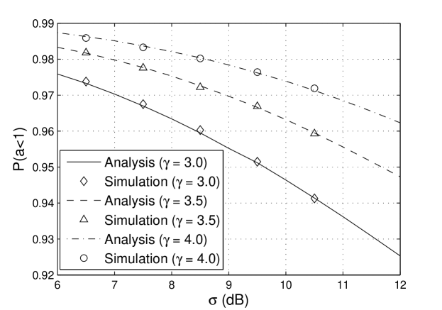
Figure 3: Probability of occurrence of the low interference regime as a function of shadow fading variance, $\sigma$ (dB) for Ray/Ray scenario.

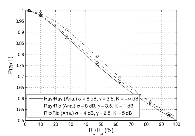
Figure 4: Probability of occurrence of the low interference regime as a function of the ratio $R_{c}/R_{p}$ for different fading scenarios. Simulation values are shown by markers on the analytical curves.

where $B(.,.)$ is the beta function. It is worth mentioning that we use $\nu_{1}=\nu_{2}=2$ and $\lambda_{1}=\lambda_{2}=2K$ while employing the above PDF to evaluate the probabilities. Although the doubly infinite sum in (20) is undesirable, satisfactory convergence was found with only $18$ terms. Hence, the approach is rapid and stable computationally. A comparison of simulated and analytical results is presented in Figs. 3 and 4. It can the seen that the analytical formulae for all the cases shown perfectly agree with the simulation results for different parameter values. A discussion of these results is presented in Sec. V.

IV An Approximation For The Power Loss Parameter

In this section we focus on the power loss parameter, $\alpha$, which governs how much of the transmit power the CR dedicates to relaying the primary message. The exact distribution of $\alpha$ appears to be rather complicated, even for fixed link gains (fixed values of $\Gamma_{cp},\Gamma_{pc},\Gamma_{pp}$ and $\Gamma_{cc}$). Hence, we consider an extremely simple approximation based on the idea that $|s||t|$ is usually small and $|s||t|>>|t|$. This approximation is motivated by the fact that the CP link is usually very weak compared to the PP link. This stems from the common scenario where the CRs will employ much lower transmit powers than the PU as the CC paths are usually much shorter. With this assumption it follows that $|t|^{2}(1+|s|^{2})$ is small and we have:

$$\sqrt{\alpha} {}={} \frac{|s|}{|t|}\Bigg{[}\frac{\big{(}1+|t|^{2}(1+|s|^{2})\big{)}^{1/2}-1}{1+|s|^{2}}\Bigg{]}$$ (21)

$${}\approx{} \frac{|s|}{|t|}\Bigg{[}\frac{1/2|t|^{2}(1+|s|^{2})}{1+|s|^{2}}\Bigg{]}$$

$${}={} \frac{|s||t|}{2}$$

$${}={} \sqrt{\alpha_{approx}}.$$

Expanding $\alpha_{approx}$ we have:

$$\alpha_{approx}=\frac{A_{p}A_{c}P_{p}P_{c}}{4N_{p}^{2}}e^{(X_{pp}+X_{cp})}r_{pp}^{-\gamma}r_{cp}^{-\gamma}|{\tilde{p}}|^{2}|{\tilde{f}}|^{2}.$$ (22)

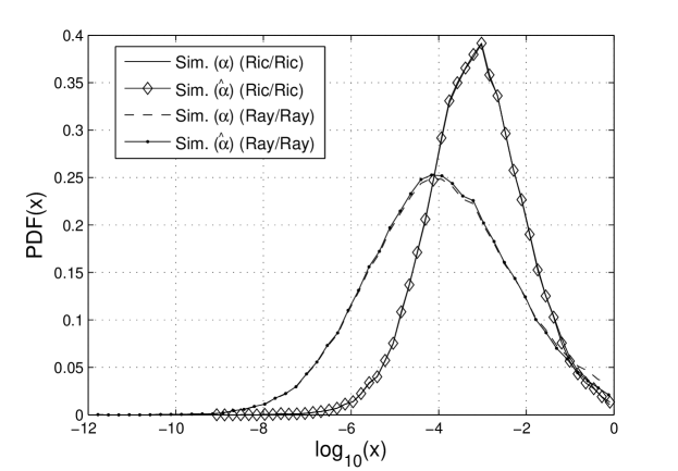
Figure 5: PDFs of $\log_{10}(\alpha)$ and its approximation $\log_{10}(\hat{\alpha})$. We use the default parameters for the Ray/Ray curve, whereas, for Ric/Ric we have taken $\sigma=4$ dB, $\gamma=2.5$ and $K=5$ dB.

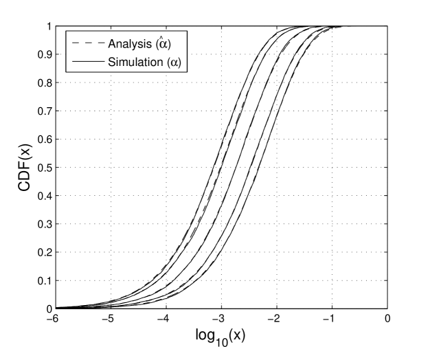
Figure 7: Comparison of the exact and analytical CDFs of the power loss factor on a logarithmic scale for fixed link gains. Results are shown for 5 drops for the case of Ray/Ray fading.

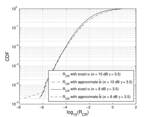
Figure 8: CDF of the CR rates with the exact $\alpha$ and the approximate $\hat{\alpha}$ for Ray/Ray fading.

This approximation is very effective for low values of $\alpha_{approx}$, but is poor for larger values since $\alpha_{approx}$ is unbounded whereas $0<\alpha<1$. To improve the approximation, we use the conditional distribution of $\alpha_{approx}$ given that $\alpha_{approx}<1$. This conditional variable is denoted, ${\hat{\alpha}}$. The exact distribution of ${\hat{\alpha}}$ is difficult for variable link gains. However, the approximation has a simple representation which leads to considerable insight into the power loss and how it relates to system parameters. For example $\alpha_{approx}$ is proportional to $|s|^{2}|t|^{2}$ so that high power loss may be caused by high values of $|s|$ or $|t|$ or moderate values of both. Now $|s|$ and $|t|$ relate to the PP and CP links respectively. Hence, the CR is forced to use high power relaying the PU message when the CP link is strong. This is obvious as the relay action needs to make up for the strong interference caused by the CR. The second scenario is that the CR has high $\alpha$ when the PP link is strong. This is less obvious, but here the PU rate is high and a substantial relaying effort is required to counteract the efforts of interference on a high rate link. This is discussed further in Section V. It is worth noting that the condition $|s||t|>>|t|$ holds good only for some specific values of channel parameters which support the assumption that the CP link is usually much weaker than the PP link. Hence, although it is motivated by a sensible physical scenario, it requires verification. Results in Figs. 5, 7 and 8 show that it works very well. For fixed link gains, the distribution of ${\hat{\alpha}}$ is:

$$P(\alpha_{approx}<x|\alpha_{approx}<1) {}={} P(\hat{\alpha}<x)$$ (23)

$${}={} \frac{P(\alpha_{approx}<x)}{P(\alpha_{approx}<1)}.$$

Thus, to compute the distribution function of $\hat{\alpha}$ we need to determine $P(\alpha_{approx}<x)$ which can be written as

$$P(\alpha_{approx}<x)=P(|s|^{2}|t|^{2}<4x).$$ (24)

Let $E(|s|^{2})=\mu_{s}$, $E(|t|^{2})=\mu_{t}$ with $\mu_{s}=P_{p}\Gamma_{pp}/N_{p}$ and $\mu_{t}=P_{c}\Gamma_{cp}/N_{p}$. Further, suppose that $U$, $V$ and $W$ are defined by $U=|\tilde{f}|^{2}$, $V=|\tilde{c}|^{2}$ and $W=|\tilde{p}|^{2}$. We wish to derive $P\big{(}WU<\frac{4x}{\mu_{s}\mu_{t}}\big{)}$, i.e., (24), subject to the condition $a<1$, which implies that $U<V/d$, where $d=(N_{c}/N_{p})(\Gamma_{cp}/\Gamma_{cc})$. Assuming $\zeta=4/\mu_{s}\mu_{t}$ the required conditional CDF is given by:

$${}P{} \bigg{(}UW<\zeta x|U<\frac{V}{d}\bigg{)}$$

$${}={} \frac{P\bigg{(}U\leq\frac{\zeta x}{W},U<\frac{V}{d}\bigg{)}}{P\big{(}U<\frac{V}{d}\big{)}}$$

$${}={} \frac{\int_{w}\int_{v}P(U<\min(\frac{\zeta x}{w},\frac{v}{d}))f_{W}(w)f_{V}(v)dvdw}{\int_{0}^{\infty}P(U<\frac{v}{d})f_{V}(v)dv}$$

$${}={} \frac{\int_{w=0}^{\infty}\int_{v=0}^{\zeta xd/w}P(U<\frac{v}{d})f_{W}(w)f_{V}(v)dvdw+\int_{w=0}^{\infty}\int_{v=\zeta xd/w}^{\infty}P(U<\frac{\zeta x}{w})f_{W}(w)f_{V}(v)dvdw}{\int_{0}^{\infty}P(U<\frac{v}{d})f_{V}(v)dv}$$

$${}={} \frac{\int_{v=0}^{\infty}\int_{w=0}^{\zeta xd/v}P(U<\frac{v}{d})f_{V}(v)f_{W}(w)dwdv+\int_{w=0}^{\infty}\int_{v=\zeta xd/w}^{\infty}P(U<\frac{\zeta x}{w})f_{W}(w)f_{V}(v)dvdw}{\int_{0}^{\infty}P(U<\frac{v}{d})f_{V}(v)dv}$$

$${}={} \frac{\int_{v=0}^{\infty}F_{W}(\zeta xd/v)F_{U}(v/d)f_{V}(v)dv+\int_{w=0}^{\infty}F_{U}(\zeta x/w)(1-F_{V}(\zeta xd/w))f_{W}(w)dw}{\int_{0}^{\infty}F_{U}(v/d)f_{V}(v)dv}.$$

In the above derivation $f_{U}(u)$ and $F_{U}(u)$ represent the PDF and CDF of $U$ respectively with similar definitions for $V$ and $W$. With the general result in (IV), the CDF of $\alpha_{approx}$ can be determined for any fading combinations across the links of the CR interference channel. In most cases where Rician fading occurs (IV) has to be computed via infinite series expansions or numerical integration. In the Rayleigh fading scenario a closed form solution is possible. Since for this case all the distribution and density functions given in (IV) are those of a standard unit mean exponential random variable, after a few algebraic manipulations (details given in Appendix II) and the substitution $\zeta=4/\mu_{s}\mu_{t}$ we have:

$$P(\alpha_{approx}<x) {}={} 1-\sqrt{\frac{16(1+d)x}{\mu_{s}\mu_{t}}}K_{1}\bigg{(}\sqrt{\frac{16(1+d)x}{\mu_{s}\mu_{t}}}\bigg{)},$$ (26)

where $K_{1}(.)$ represents the modified Bessel function of the second kind. Using the expression given in (26), the CDF of $\hat{\alpha}$ follows from (23). Note that the CDF of $R_{CR}$ in (5) can easily be obtained in the form of a single numerical integral for fixed link gains as below:

$$P(R_{CR}<x) {}={} P\bigg{(}|c|^{2}(1-\alpha)<(2^{x}-1)\frac{N_{c}}{P_{c}}\bigg{)}$$ (27)

$${}={} E\bigg{[}P\bigg{(}\alpha>1-\frac{(2^{x}-1)N_{c}}{|c|^{2}P_{c}}\bigg{)}\bigg{]}$$

$${}={} \int_{0}^{\infty}\bigg{(}1-F_{\alpha}\bigg{(}1-\frac{(2^{x}-1)N_{c}}{|c|^{2}P_{c}}\bigg{)}\bigg{)}f_{c}(c)dc$$

where $F_{\alpha}(.)$ is the CDF of $\alpha$ in (26) and $f_{c}(c)$ is the PDF of $c$.

V Results

In the results section, the default parameters are $\sigma=8$ dB, $\gamma=3.5$, $R_{0}=1$ m, $R_{c}=100$ m, $R_{p}=1000$ m and $N_{p}=N_{c}=P_{p}=P_{c}=1$. The parameter $A_{p}$ is determined by ensuring that the PP link has an SNR $\geq 5$ dB 95% of the time in the absence of any interference. Similarly, assuming that both PU and CR devices have same threshold power at their cell edges, the constant $A_{c}=A_{p}(R_{p}/R_{c})^{-\gamma}$. Unless otherwise stated these parameters are used in the following.

V-A Low interference regime

In Figs. 3 and 4 we show that the low interference regime, $a<1$, is the dominant scenario when the CR coverage area is small compared to that of PU. For typical values of $\gamma\in[3,4]$ and $\sigma\in[6,12]$ dB we find that $P(a<1)$ is usually well over 90% when $R_{c}$ is less than 20% of $R_{p}$. As expected, when $R_{c}$ approaches $R_{p}$ the probability drops and reaches $P(a<1)=0.5$ when $R_{c}=R_{p}$. Note that this is only the case when all the channel parameters are the same for the CC and CP links. From Fig. 4 we observe that the results are reasonably insensitive to the type of fast fading. This is due to the lesser importance of the fast fading compared to the large effects of shadowing and path loss. Figure 3 also verifies the analytical result in (15).

The relationship between $P(a<1)$ and the system parameters is easily seen from (4) which contains the term $\big{(}r_{cc}/r_{cp}\big{)}^{\gamma/2}\exp\big{(}(X_{cp}-X_{cc})/2\big{)}$. When $R_{c}<<R_{p}$, this term decreases dramatically as $\gamma$ increases (i.e., $P(a<1)$ increases) and as $\sigma$ increases the term increases (hence $P(a<1)$ decreases). Also, as $R_{c}$ increases $r_{cc}/r_{cp}$ tends to increase which in turn decreases $P(a<1)$. When $R_{c}\approx R_{p}$ the low and high interference scenarios occur with similar frequency (Fig. 4). This may be a relevant system consideration if CRs were to be introduced in cellular bands where the cellular hot spots, indoor micro-cells and CRs will have roughly the same coverage radius. Note that $a$ is independent of the transmit power, $P_{c}$. These conclusions are all verified in Figs. 3 and 4.

V-B Statistics of the power loss parameter, $\alpha$

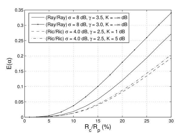
Figure 6: Mean value of the power loss parameter, $\alpha$, as a function of the ratio $\frac{R_{c}}{R_{p}}$ for different fading scenarios.

Figures 5-7 all focus on the properties of $\alpha$. Figure 5 shows that the probability density function (PDF) of $\alpha$ is extremely well approximated by the PDF of $\hat{\alpha}$ in both Rayleigh and Rician fading channels. In Fig. 6 we see that $E(\alpha)$ increases with increasing values of $R_{c}/R_{p}$ and decreasing values of $\gamma$. This can be seen from (22) where $\alpha_{approx}$ contains a $(r_{pp}r_{cp})^{-\gamma}$ term which increases as $\gamma$ decreases, thus increasing the mean value of $\alpha$. The increase of $E(\alpha)$ with $R_{c}$ follows from the corresponding increase in $P_{c}$ to cater for larger $R_{c}$ values. Increasing the line of sight (LOS) factor tends to increase $E(\alpha)$ although the effect is minor compared to changes in $\gamma$, $\sigma$ or $R_{c}/R_{p}$. In Fig. 6 we have limited $R_{c}/R_{p}$ to a maximum of $30\%$ as beyond this value the high interference regime is also present with a non-negligible probability. In Fig. 7 we see the analytical CDF in (26) verified by simulations for five different scenarios of fixed link gains (simply the first five simulated values of $\Gamma_{pp}$ and $\Gamma_{cp}$). Note that in the different curves each correspond to a random drop of the PU and CR transmitters. This fixes the distance and shadow fading terms in the link gains in (2), thereby the remaining variation in (1) is only Rayleigh. By computing a large number of such CDFs and averaging them over the link gains a single CDF can be constructed. This approach can be used to find the PDF of $\hat{\alpha}$ as shown in Fig. 5. Note that the curves in Fig. 7 do not match exactly since the analysis is for $\hat{\alpha}$ and the simulation is for $\alpha$.

V-C CR rates

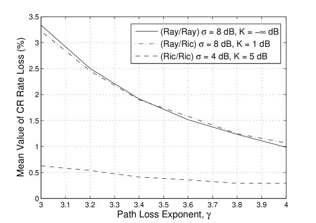
Figure 9: Mean value of the CR rate loss as a function of $\gamma$ for different fading conditions.

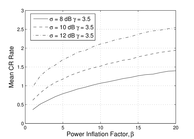
Figure 10: Variation of the mean CR rate with the power inflation factor, $\beta$ for Ray/Ray fading case.

Figures 8-10 focus on the CR rate $R_{CR}$. Figure 8 demonstrates that the use of $\hat{\alpha}$ is not only accurate for $\alpha$ but also leads to excellent agreement for the CR rate, $R_{CR}$. This agreement holds over the whole range and for all typical parameter values. Figure 9 shows the % loss given by $[R_{CR}(\alpha=0)-R_{CR}(\alpha)]/[R_{CR}(\alpha=0)]\%$. The loss decreases as $\gamma$ increases, as discussed above, and increases with $\sigma$. From (22) it is clear that increasing $\sigma$ lends to larger values of $\exp(X_{pp}+X_{cp})$ which in turn increases $\alpha$ and the rate loss. Note that the rate loss is minor for $\sigma\in[8-10]$ dB with $R_{c}=R_{p}/10$. In a companion paper [17], we show that the interference to the PU increases with $\sigma$ and decreases with $\gamma$. These results reinforce this observation, i.e., when the PU suffers more interference ($\sigma$ is larger) the CR has to devote a higher part of its power to the PU. Consequently the percentage rate loss is higher. Again the effect of $K$, the LOS factor, is minor compared to $\gamma$ and $\sigma$.

Finally, in Fig. 10 we investigate the gains available to the CR through increasing transmit power. The original transmit power, $P_{c}$, is scaled by $\beta$ and the mean CR rate is simulated over a range of $\beta$ values. Due to the relaying performed by the CR, the PU rate is unaffected by the CR for any values of $\beta$ and so the CR is able to boost its own rate with higher transmit power. Clearly the increased value of $\alpha$ for higher values of $\beta$ is outweighed by the larger $P_{c}$ value and so the CR does achieve an overall rate gain. In a very coarse way these results suggest that multiple CRs may be able to co-exist with the PU since the increased interference power might be due to several CRs and the rate gain might be spread over several CRs. Of course, this conclusion is speculative as the analysis is only valid for a single CR.

VI Conclusion

In this paper we derive the probability that the “low interference regime” holds and demonstrate the conditions under which this is the dominant scenario. We show that the probability of the low interference regime is significantly influenced by the system geometry. When the CR coverage radius is small relative to the PU radius, the low interference regime is dominant. On the other hand, when the CR coverage radius approaches a value similar to the PU coverage radius, the low and high interference regimes both occur with roughly equal probability. In addition, we have derived a simple, accurate approximation to $\alpha$ which gives considerable insight into the system capacity. The $\alpha$ approximation shows that the mean value of $\alpha$ is increased by small values of $\gamma$, large CR coverage zones and higher $\sigma$ values. This in turn decreases CR rates due to small values of $\gamma$, large CR coverage zones and $\sigma$. The effect of the LOS strength is shown to be minor and all results appear to be insensitive to the type of fast fading. Finally, we have shown that the CR can increase its own rate with higher transmit powers, although the relationship is only slowly increasing as expected.

Appendix A

The variable $r_{cc}$ represents the distance of the CR link where the receiver is uniformly located in an annulus of dimension $[R_{0},R_{c}]$ around the transmitter. Similarly, $r_{cp}$ describes the the distance of the CR transmitter to the PU receiver where the CR transmitter is uniformly located in an annulus of dimension $[R_{0},R_{p}]$ around the PU receiver. To evaluate the distribution of $r_{cc}/r_{cp}$, we proceed as:

$$P(r_{cc}<xr_{cp}) {}={} E_{r_{cp}}[P(r_{cc}<xr_{cp}|r_{cp})]$$ (28)

$${}={} \int_{\alpha}^{\beta}\frac{2r_{cp}(x^{2}r_{cp}^{2}-R_{0}^{2})}{(R_{c}^{2}-R_{0}^{2})(R_{p}^{2}-R_{0}^{2})}\>dr_{cp}$$

$${}={} \frac{0.5x^{2}(\beta^{4}-\alpha^{4})-R_{0}^{2}(\beta^{2}-\alpha^{2})}{(R_{c}^{2}-R_{0}^{2})(R_{p}^{2}-R_{0}^{2})},$$

where we have used the facts that the PDF of the variable $r_{cp}$ is given by $2r_{cp}/(R_{p}^{2}-R_{0}^{2})$ and that $P(r_{cc}<xr_{cp})=(x^{2}r_{cp}^{2}-R_{0}^{2})/(R_{c}^{2}-R_{0}^{2})$. A little inspection reveals that the random variable $r_{cp}$ takes on the values $\alpha<x\leq\beta$ corresponding to the three different ranges of $x$ as below:

• for $R_{0}/R_{p}<x<R_{c}/R_{p}$, $r_{cp}$ ranges from $\alpha=R_{0}/x$ to $\beta=R_{p}$,

• for $R_{c}/R_{p}<x<1$, $r_{cp}$ has a range from $\alpha=R_{0}/x$ to $\beta=R_{c}/x$, and

• for $1<x<R_{c}/R_{0}$, $r_{cp}$ spans a range from $\alpha=R_{0}$ to $\beta=R_{c}/x$.

Hence, using the above ranges of $x$ and $r_{cp}$ in (28), some mathematical manipulations lead to (7).

Appendix B

When there is Rayleigh fading in all links of the CR interference channel, the distribution and density functions given in (IV) are those of a standard unit mean exponential random variable. Thus, with this substitution in (IV) we get:

$$P\bigg{(}UW<\zeta x|U<\frac{V}{d}\bigg{)} {}={} \frac{\int_{0}^{\infty}(1-e^{-\zeta xd/v})(1-e^{-v/d})e^{-v}dv+\int_{0}^{\infty}(1-e^{-\zeta x/w})e^{-w}e^{-\zeta xd/w}dw}{\int_{0}^{\infty}(1-e^{-v/d})e^{-v}dv}$$ (29)

$${}={} 1+\frac{\int_{0}^{\infty}e^{-\zeta xd/v-v(1+1/d)}dv-\int_{0}^{\infty}e^{-w-\zeta/w(x+xd)}dw}{1-d/(1+d)}$$

$${}={} 1+(d+1)\bigg{[}\int_{0}^{\infty}e^{-\zeta xd/v-v(1+d)/d}dv-\int_{0}^{\infty}e^{-w-\zeta x(1+d)/w}dw\bigg{]}$$

$${}\stackrel{{\scriptstyle a}}{{=}}{} 1+(d+1)\bigg{[}\int_{0}^{\infty}e^{-\zeta xd/v-v(1+d)/d}dv-(1+d)/d\int_{0}^{\infty}e^{-v(1+d)/d-\zeta xd/v}dv\bigg{]}$$

$${}={} 1-(d+1)/d\int_{0}^{\infty}e^{-\zeta xd/v-v(1+d)/d}dv$$

$${}\stackrel{{\scriptstyle b}}{{=}}{} 1-\int_{0}^{\infty}e^{-\zeta x(1+d)/t-t}dt.$$

where in both $a$ and $b$ above we have used the substitutions $w=v(1+d)/d$ and $t=v(1+d)/d$ respectively. Now using $\zeta=4/\mu_{s}\mu_{t}$ and evaluating the integral in the last equality using a standard result in [18] we arrive at (26).

References

- [1] M. A. McHenry, “NSF Spectrum Occupancy Measurements Project Summary,” Shared Spectrum Company, Tech. Rep., 2005.
- [2] “Spectrum Policy Task Force Report (ET Docket-135),” Federal Communications Comsssion, Tech. Rep., 2002. [Online]. Available: http://hraunfoss.fcc.gov/edocs˙public/attachmatch/DOC-228542A1.pdf
- [3] A. Ghasemi and E. S. Sousa, “Spectrum sensing in cognitive radio networks: requirements, challenges and design trade-offs [cognitive radio communications],” IEEE Communications Magazine, vol. 46, no. 4, pp. 32–39, April 2008.
- [4] R. Tandra, S. M. Mishra, and A. Sahai, “What is a spectrum hole and what does it take to recognize one?” Proceedings of the IEEE special issue on Cognitive Radio, vol. 97, no. 5, pp. 824–848, May 2009.
- [5] A. Ghasemi and E. S. Sousa, “Fundamental limits of spectrum-sharing in fading environments,” IEEE Transactions on Wireless Communications, vol. 6, no. 2, pp. 649–658, Feb. 2007.
- [6] N. Devroye, P. Mitran, and V. Tarokh, “Achievable rates in cognitive radio channels,” IEEE Transactions on Information Theory, vol. 52, no. 5, pp. 1813–1827, May 2006.
- [7] I. Maric, A. Goldsmith, G. Kramer, and S. S. (Shitz), “On the capacity of interference channels with one cooperating transmitter,” European Transactions on Telecommunications, vol. 19, pp. 405–420, Apr. 2008.
- [8] A. Jovicic and P. Viswanath, “Cognitive radio: An information-theoretic perspective,” in Proc. IEEE International Symposium on Information Theory, July 2006, pp. 2413–2417.
- [9] J. Jiang and Y. Xin, “A new achievable rate region for the cognitive radio channel,” in Proc. IEEE International Conference on Communications, May 2008, pp. 1055–1059.
- [10] W. Wu, S. Vishwanath, and A. Arapostathis, “Capacity of a class of cognitive radio channels: Interference channels with degraded message sets,” IEEE Transactions on Information Theory, vol. 53, no. 11, pp. 4391–4399, Nov. 2007.
- [11] G. Kramer, “Review of rate regions for interference channels,” in Proc. International Zurich Seminar on Communications, 2006, pp. 162–165.
- [12] M. Costa, “Writing on dirty paper (corresp.),” IEEE Transactions on Information Theory, vol. 29, no. 3, pp. 439–441, May 1983.
- [13] M. Vu, N. Devroye, and V. Tarokh, “On the primary exclusive regions in cognitive networks,” IEEE Transactions on Wireless Communications, accepted.
- [14] A. Papoulis and S. U. Pillai, Probability, Random Variables and Stochastic Processes, 4th ed. New York: McGraw Hill, 2002.
- [15] H. A. Suraweera, J. Gao, P. J. Smith, M. Shafi, and M. Faulkner, “Channel capacity limits of cognitive radio in asymmetric fading environments,” in Proc. IEEE International Conference on Communications, May 2008, pp. 4048–4053.
- [16] N. L. Johnson, S. Kutz, and N. Balakrishnan, Continuous Univariate Distributions, vol. 2, 2nd ed. New York: Wiley, 1995.
- [17] M. F. Hanif, M. Shafi, P. J. Smith, and P. Dmochowski, “Interference and deployment issues for cognitive radio systems in shadowing environments,” to appear in Proc. IEEE ICC, June 2009.
- [18] I. S. Gradshteyn and I. M. Ryzhik, Table of Integrals, Series, and Products, 7th ed. California USA: Academic Press, 2007.