Indirect Influences

Abstract

We introduce the PWP method for counting indirect influences, and compare it with three well-known methods, namely, MICMAC, Heat Kernel, and PageRank. We provide combinatorial as well as probabilistic interpretation for the PWP method.

1 Introduction

Our goal in this note is to compare four alternative approaches to count indirect influences. Two of these approaches, the MICMAC and PageRank methods, are well-tested and each possesses a host of real-life applications. The Heat Kernel method has found interesting mathematical applications. We believe that the PWP method, while still in its infancy, may also be useful in a variety of contexts. Our guide for the definition of the PWP method is threefold:

• Direct influences generate, by concatenation, indirect influences.

• All indirect influences arise from the concatenation of direct influences.

• Longer concatenations exert a lesser indirect influence.

We consider a discrete scenario where the variables involved are indexed, and often identified, with the set $[n]=\{1,2,...,n\}$ for some $n\in\mathbb{N}_{+}.$ We assume that direct influences among our variables are encoded into a $\mathbb{R}$-weighted directed graph, without multiple edges, with $[n]$ as its set of vertices. Thus a direct influence from the variable $j\in[n]$ on the variable $i\in[n]$ corresponds with an edge of weight $D_{ij}$ from vertex $j$ to vertex $i$. As usual the graph is encoded into the matrix of direct influences $D$, which is such that $D_{ij}$ is the weight of the edge going from $j$ to $i$, if there is one, and $D_{ij}=0$ otherwise. Our problem consists in evaluating the indirect influences between the variables, i.e. finding the matrix $T$ such that $T_{ij}$ measures the indirect influence of variable $j$ on variable $i$. In this work we make a comparative analysis of four possible definitions for $T$.

2 MICMAC

The MICMAC method, introduced by Godet [5], works as follows. Let $D$ be the matrix associated with the graph of direct influences. The graph of indirect influences is represented by the matrix $T=D^{k},$ where $k$ is a fixed small natural number, say $4$ or $5$. The vector of indirect dependencies $d=(d_{1},....d_{n})$ and the vector indirect of influences $f=(f_{1},....f_{n})$, are such that their coefficients $d_{j}$ and $f_{j}$ are given, respectively, by:

$$d_{j}=\sum_{i=1}^{n}T_{ji}\ \ \ \ \ \ \ \mbox{ and }\ \ \ \ \ \ \ f_{j}=\sum_{i=1}^{n}T_{ij}.$$ (1)

Thus $(d_{j},f_{j})$ is equal to the $(\mathrm{in},\mathrm{out})$-degree of the vertex $j$ in the graph of indirect influences. The numbers $d_{j}$ and $f_{j}$ encode valuable information, for example, the most influential variable is the one for which $f_{j}$ reaches its highest value.

3 PageRank

The celebrated method PageRank [2] for computing indirect dependencies has already revolutionized the world of internet search engines trough the remarkable success of Google. The mathematics encoding the basic structure behind PageRank are however surprisingly simple. With hindsight we observe that PageRank differs from MICMAC in three main ideas:

• Normalization of influences, i.e. use of column stochastic matrices.

• Use of complete graphs, i.e. graphs whose associated matrice have no vanishing entries.

• Taking infinite potencies of matrices.

Let $D$ be the $n\times n$ matrix of direct influences whose entries are non-negative real numbers. Assume that the sum of the entries of each column of $D$ is either $0$ or $1$. With PageRank the matrix of indirect influences $T=T(D)$ is computed as follows:

$$T=T(D)=\lim_{k\to\infty}\left[p\overline{D}+(1-p)E_{n}\right]^{k}$$ (2)

where:

• The parameter $0<p<1$ is a chosen number close to $1$, say $p=0.86.$

• The matrix $\overline{D}$ is obtained from $D$ by replacing the entries of each zero column of $D$ by $\frac{1}{n}$.

• The matrix $E_{n}$ has all of its entries equal to $\frac{1}{n}$.

For the web application the matrix $D$ is constructed as follows. Consider the web graph whose set of vertices $[n]$ represents the set of all web pages in the world wide web. There is an edge from page $j$ to page $i$ in the web graph if an hyperlink to page $i$ appears in the content of page $j.$ The matrix $D$ of direct influences is given by:

$$D_{ij}=\left\{\begin{array}[]{l}\frac{1}{\mathrm{out}(j)}\ \ \text{ if there is an edge from}\ j\ \text{to}\ i,\\ \ \ 0\ \ \ \ \ \ \ \text{if there is no edge from}j\ \text{to}\ i.\\ \end{array}\right.$$

Since $p\overline{D}+(1-p)E_{n}$ is a column stochastic matrix, then so is $T$ and thus the vector of influences for $T$ is $(1,...,1)$. The entries of the vector $\frac{d}{n}=\frac{1}{n}(d_{1},...,d_{n})$, where $d$ is the vector of dependencies of $T$ whose coordinates are given by (1), yields the PageRank number of each web page. The greater the PageRank number of a page the greater its importance. By construction $p\overline{D}+(1-p)E_{n}$ is the transition matrix of a primitive irreducible Markov chain [6]. Therefore the vector of indirect dependencies $d$ is an eigenvector of $T$ with eigenvalue $1$, i.e. we have that

$$Td^{t}=d^{t}.$$

Moreover, the matrix $T$ can be computed in terms of $d$ as follows

$$T=\left(\frac{d^{t}}{n}\ \ \frac{d^{t}}{n}\ \ ....\ \ \frac{d^{t}}{n}\right).$$

4 Heat Kernel

The Heat Kernel method of Chung [3] proceeds as follows. Just as MICMAC depends on a parameter $k$, and PageRank on the parameter $p$, the Heat Kernel method depends on a parameter $\lambda$, a fixed positive real number. Given $D$, the matrix of direct influences, the matrix $T=T(D)$ of indirect influences is given for a fixed parameter $\lambda>0$ by

$$T=T(D)=e^{\lambda(D-I)},$$

where $I$ is the identity matrix of the appropriate size. Note that when $D=0$, i.e. in the absence of direct influences, the matrix of indirect influences $T=T(0)$ is not the zero matrix, since each vertex self-influences itself. Indeed, in this case we have that

$$T=T(0)=e^{-\lambda}I.$$

5 PWP

Let us introduce the PWP method for counting indirect influences. Unlike PageRank, the PWP method can be applied to any matrix of direct influences, even matrices with negatives entries. Theorem 3 below shows that whereas MICMAC focuses on paths of a fixed length $k$, and PageRank focuses on infinite long paths, the Heat Kernel and PWP methods take into account paths of various lengths. The PWP method avoids the self-influences that are included, by default, in the Heat Kernel method.

In a nutshell the PWP method can described as follows. As with the Heat Kernel, we fixed a parameter $\lambda>0$. Assume we are given the matrix $D$ of direct influences, and let $T$, the matrix of indirect influences, be given by

$$T=T(D)=\frac{e^{\lambda D}-I}{e^{\lambda}-1}=\frac{e_{+}^{\lambda D}}{e_{+}^{\lambda}},$$

where

$$e_{+}^{x}=e^{x}-1=\sum_{k=1}^{\infty}\frac{x^{k}}{k!}.$$

Note that $D^{k}=\frac{\partial^{k}}{\partial\lambda^{k}}\left(e_{+}^{\lambda}T\right)|_{\lambda=0}$, for $k\geq 1$, and thus in principle one can compute the MICMAC matrix of indirect influences from the PWP matrix of indirect influences.

Let us consider a rather trivial example which however highlights some of the differences between the four methods. Let $\mathrm{L}_{2}$ be the graph $1\rightarrow 2,\$ i.e. the graph with vertex set $[2]$ and a unique edge from $1$ to $2$.

The MICMAC matrix of indirect influences in this case vanishes for $k\geq 2$, thus no vertex influences or depends on another vertex.

PageRank makes $1$ the most influential vertex, and $2$ the most dependent vertex. Note the difference with MICMAC. It assigns a non-vanishing dependency of vector $1$ on vector $2$. It also assigns a non-vanishing dependency of $1$, respectively $2$, on itself.

Heat Kernel makes $1$ the most influential vertex, and $2$ the most dependent vertex. It assigns a vanishing dependency of $1$ on $2$. Note the difference with PageRank. It assigns a non-vanishing dependency of $1$, respectively $2$, on itself.

With PWP the only non-vanishing entry of the matrix $T$ is

$$T_{12}=\frac{\lambda}{e^{\lambda}-1},$$

thus making $1$ the most influential vertex, and $2$ the most dependent vertex. Note the differencie with MICMAC. Vertex $2$ does not exert any influence on vertex $1$, unlike with PageRank. There is not self-influence of a vertex on itself, which illustrates the difference between the PWP and Heat Kernel methods.

Note that the indirect influence of vertex $1$ over vertex $2$ is given by

$$\frac{\lambda}{e^{\lambda}-1}=\sum_{k=0}^{\infty}B_{k}\frac{\lambda^{k}}{k!},$$

where the coefficients $B_{k}$ are the so-called Bernoulli numbers. See [4] for an explicit definition and a combinatorial interpretation for the Bernoulli numbers. Note also that

$$\frac{\lambda}{e^{\lambda}-1}\leq 1,\ \ \ \ \ \ \ \frac{\lambda}{e^{\lambda}-1}\rightarrow 1\ \ \ \mbox{as}\ \ \ \lambda\rightarrow 0,\ \ \ \ \ \ \text{and}\ \ \ \ \ \frac{\lambda}{e^{\lambda}-1}\rightarrow 0\ \ \ \text{as}\ \ \ \lambda\rightarrow\infty.$$

Therefore, the indirect influence that $1$ exerts over $2$ is lesser than the original direct influence, it approaches its original value when $\lambda$ approaches $0$, and it is negligible when $\lambda$ is a large number. In other words, the direct influence that $1$ exerts over $2$ becomes less relevant as $\lambda$ increases, since with the PWP method the paths of length close to $\lambda$ are the most relevants.

Next result states some of the basic properties of the map $D\rightarrow T(D)$ and provides a probabilistic interpretation for the PWP method.

Theorem 1.

Let $T=T(D)$ be the matrix of indirect influences with the PWP method.

1. If $D=0$, then $T(D)=0.$     $T(D^{t})=T(D)^{t}.$

2. $T(QCQ^{-1})=QT(C)Q^{-1}$.

3. Let $D_{1}\oplus D_{2}\in M_{m}(\mathbb{R})\oplus M_{n}(\mathbb{R})\subseteq M_{m+n}(\mathbb{R})$, then $T(D_{1}\oplus D_{2})=T(D_{1})\oplus T(D_{2})$.

4. If $D$ is a column stochastic matrix, then $T(D)$ is a column stochastic matrix.

5. If $[D_{1},D_{2}]=0$, then we have that

   $$T(D_{1}+D_{2})=e_{+}^{\lambda}T(D_{1})T(D_{2})+T(D_{1})+T(D_{2}).$$

6. Let $D\in M_{n}(\mathbb{R})$, then $T(D)$ is the expected matrix of the random matrix $\widehat{D},$ where

   1. $\widehat{D}:\mathbb{N}_{+}\longrightarrow M_{n}(\mathbb{R})$ is the random matrix given by $\widehat{D}(k)=D^{k}$.

   2. $\mathbb{N}_{+}$ is the probability space with probability function $p(k)=\frac{\lambda^{k}}{e_{+}^{\lambda}k!}$.

Proof.

1. $T(D^{t})=\frac{e_{+}^{\lambda D^{t}}}{e_{+}^{\lambda}}=\left(\frac{e_{+}^{\lambda D}}{e_{+}^{\lambda}}\right)^{t}=T(D)^{t}.$
2. $T(QDQ^{-1})=\frac{e_{+}^{\lambda QDQ^{-1}}}{e_{+}^{\lambda}}=\frac{Qe_{+}^{\lambda D}Q^{-1}}{e_{+}^{\lambda}}=T(D).$
3. $T(D_{1}\oplus D_{2})=\frac{e_{+}^{\lambda(D_{1}\oplus D_{2})}}{e_{+}^{\lambda}}=\frac{e_{+}^{\lambda D_{1}}\oplus\ e_{+}^{\lambda D_{2}}}{e_{+}^{\lambda}}=\frac{e_{+}^{\lambda D_{1}}}{e_{+}^{\lambda}}\oplus\frac{e_{+}^{\lambda D_{1}}}{e_{+}^{\lambda}}=T(D_{1})\oplus T(D_{2}).$
4. Let $c_{j}$ be the linear functional on matrices such that $c_{j}(S)$ is the sum of the entries of the $j$-column of the matrix $S$, i.e. $c_{j}(S)=\sum_{i=1}^{n}S_{ij}.$ A matrix $S$ is column stochastic if its entries are non-negative and $c_{j}(S)=1$ for all $j$. It is easy to check that if $S$ is column stochastic so is $S^{k}$ for $k\geq 1$. Assume that $D$ is a column stochastic matrix, then

$$c_{j}(T(D))=c_{j}\left(\frac{e_{+}^{\lambda D}}{e_{+}^{\lambda}}\right)=\frac{\sum_{k=1}^{\infty}\frac{\lambda^{k}c_{j}(D^{k})}{k!}}{e_{+}^{\lambda}}=\frac{\sum_{k=1}^{\infty}\frac{\lambda^{k}}{k!}}{e_{+}^{\lambda}}=\frac{e_{+}^{\lambda}}{e_{+}^{\lambda}}=1.$$

5. Assume that $[D_{1},D_{2}]=0$, then we have that

$$T(D_{1}+D_{2})=\frac{e_{+}^{\lambda(D_{1}+D_{2})}}{e_{+}^{\lambda}}=\frac{e^{\lambda(D_{1}+D_{2})}-I}{e_{+}^{\lambda}}=\frac{e^{\lambda D_{1}}e^{\lambda D_{2}}-I}{e_{+}^{\lambda}}=\frac{(e_{+}^{\lambda D_{1}}+I)(e_{+}^{\lambda D_{2}}+I)-I}{e_{+}^{\lambda}}$$

$$=\frac{e_{+}^{\lambda D_{1}}e_{+}^{\lambda D_{2}}}{e_{+}^{\lambda}}\ +\ \frac{e_{+}^{\lambda D_{1}}}{e_{+}^{\lambda}}\ +\ \frac{e_{+}^{\lambda D_{2}}}{e_{+}^{\lambda}}=e_{+}^{\lambda}T(D_{1})T(D_{2})\ +\ T(D_{1})\ +\ T(D_{2}).$$

6. By definition the expected matrix $E\widehat{D}$ of the random matrix $\widehat{D}$ is given by

$$E\widehat{D}=\sum_{k=1}^{\infty}\widehat{D}(k)p(k)=\sum_{k=1}^{\infty}D^{k}\frac{\lambda^{k}}{e_{+}^{\lambda}k!}=\frac{\sum_{k=1}^{\infty}\frac{(\lambda D)^{k}}{k!}}{e_{+}^{\lambda}}=\frac{e_{+}^{\lambda D}}{e_{+}^{\lambda}}=T(D).$$

∎

Recall that the Poisson probability $P$ on $\mathbb{N}$ is given by $P(k)=e^{-\lambda}\frac{\lambda^{k}}{k!}.$ Let again $p$ be the probability on $\mathbb{N}_{+}$ given by $p(k)=\frac{\lambda^{k}}{e_{+}^{\lambda}k!}$.

Proposition 2.

With the above notation we have that:

1. For $k\geq 1$ we have that $p(k)=\frac{P(k)e^{\lambda}}{e^{\lambda}-1}$.

2. Let $X$ be a random variable with distribution $p$, then

   $$EX=\frac{\lambda e^{\lambda}}{e^{\lambda}-1},\ \ \ \ \ \ EX^{2}=\frac{(\lambda^{2}+\lambda)e^{\lambda}}{e^{\lambda}-1},\ \ \ \ \ \ \mbox{and}\ \ \ \ \ \ VX=\frac{\lambda e^{2\lambda}-(\lambda^{2}+\lambda)e^{\lambda}}{(e^{\lambda}-1)^{2}}.$$

3. We have that

   $$p\left(\left|X-\frac{\lambda e^{\lambda}}{e^{\lambda}-1}\right|\geq c\right)\leq\frac{\lambda e^{2\lambda}-(\lambda^{2}+\lambda)e^{\lambda}}{c^{2}(e^{\lambda}-1)^{2}}.$$

Proof.

1. is a trivial calculation, and 2. follows from 1. and the well-known fact that if $X$ is a Poisson random variable then

$$EX=\lambda\ \ \ \ \text{and}\ \ \ \ VX=\lambda^{2}+\lambda.$$

3. Direct consequence of the Chebyschev’s inequality. ∎

In order to provide a combinatorial interpretation for the MICMAC, PageRank, Heat Kernel and PWP methods we need a few definitions, see for example [1]. Let $\mathbb{R}$-set be the category of $R$-weighted finite sets, i.e. the category whose objects are pairs $(x,\omega)$ where $x$ is a finite set and $\omega:x\rightarrow\mathbb{R}$ is a map. A morphism in $\mathbb{R}$-Set from $(x_{1},\omega_{1})$ to $(x_{2},\omega_{2})$ is a map $\alpha:x_{1}\rightarrow x_{2}$ such that $\omega_{1}=\omega_{2}\circ\alpha.$ $\mathbb{R}$-set is a distributive category provided with a natural valuation map

$$|\ \ |:\mathbb{R}\text{-}\mathrm{set}\rightarrow\mathbb{R}$$

given by

$$|x,\omega|=\sum_{i\in x}\omega(i).$$

Note that the definition above may, sometimes, be applied for some infinite sets as well. If $e$ is an edge of a directed graph we denote by $se$ and $te$ the starting point and the endpoint of $e$, respectively. A path $\gamma$ of length $k$ from a vertex $j$ to a vertex $i$ in a graph is a sequence of edges $\gamma=(\gamma_{1},....,\gamma_{k})$ such that $s\gamma_{1}=j$, $t\gamma_{i}=s\gamma_{i+1}$ for $1\leq i<k$ and $t\gamma_{k}=i.$ We let $P(i,j)$ be the set of all paths from $j$ to $i$, and $P_{k}(i,j)$ be the set of paths of length $k$ from $j$ to $i$.

We assume that the graph of direct influences has associated matrix $D$. In our applications we use the $\mathbb{R}$-weighted sets $(P_{k}(i,j),\omega)$, $(P_{k}(i,j),\rho)$, $(P(i,j),\sigma)$ and $(P(i,j),\tau)$ where the weights $\omega$, $\rho$, $\sigma$ and $\tau$ are given, respectively, on a path $\gamma=(\gamma_{1},....,\gamma_{k})$ in the graph of direct influences by

$$\omega(\gamma) = \prod_{i=1}^{k}D_{t\gamma_{i},s\gamma_{i}},$$

$$\rho(\gamma) = \prod_{i=1}^{k}\left(p\overline{D}+(1-p)E_{n}\right)_{t\gamma_{i},s\gamma_{i}},$$

$$\sigma(\gamma) = \sigma_{k}(\gamma)\frac{\lambda^{k}}{k!}=\prod_{i=1}^{k}(D-I)_{t\gamma_{i},s\gamma_{i}}\frac{\lambda^{k}}{k!}.$$

$$\tau(\gamma) = \tau_{k}(\gamma)\frac{\lambda^{k}}{e_{+}^{\lambda}k!}=\left(\prod_{i=1}^{k}D_{t\gamma_{i},s\gamma_{i}}\right)\frac{\lambda^{k}}{e_{+}^{\lambda}k!}.$$

The following result provides combinatorial interpretation for the MICMAC, PageRank, Heat Kernel and the PWP methods.

Theorem 3.

1. Let $T$ be the MICMAC matrix of indirect influences. Then $T_{ij}=|P_{k}(i,j),\omega|$.

2. Let $T$ be the PageRank matrix of indirect influences. Then $T_{ij}=\lim_{k\to\infty}|P_{k}(i,j),\rho|$.

3. Let $T$ is the Heat Kernel matrix of indirect influences. Then

   $$T_{ij}=|P(i,j),\sigma|=\sum_{k=0}^{\infty}|P_{k}(i,j),\sigma_{k}|\frac{\lambda^{k}}{k!}.$$

4. Let $T$ is the PWP matrix of indirect influences. Then

   $$T_{ij}=|P(i,j),\tau|=\sum_{k=1}^{\infty}|P_{k}(i,j),\tau_{k}|\frac{\lambda^{k}}{e_{+}^{\lambda}k!}.$$

Proof.

1. The MICMAC matrix $T$ is equal to $D^{k}$, thus we have that

$$T_{ij}=D^{k}_{ij}=\sum_{s_{1},....,s_{k-1}=1}^{n}D_{is_{1}}....D_{s_{k-1}j}=$$

$$\sum_{(\gamma_{1},...,\gamma_{k})\in P_{k}(i,j)}\prod_{i=1}^{k}D_{t\gamma_{i},s\gamma_{i}}=\sum_{\gamma\in P_{k}(i,j)}\omega(\gamma)=|P_{k}(i,j),\omega|.$$

2. The PageRank matrix $T$ is given $\mbox{lim}_{k\to\infty}\left[p\overline{D}+(1-p)E_{n}\right]^{k}$, thus we have that

$$T_{ij} = \lim_{k\to\infty}\left[p\overline{D}+(1-p)E_{n}\right]_{ij}^{k}$$

$$= \lim_{k\to\infty}\sum_{s_{1},....,s_{k-1}=1}^{n}\left[p\overline{D}+(1-p)E_{n}\right]_{is_{1}}....\left[p\overline{D}+(1-p)E_{n}\right]_{s_{k-1}j}$$

$$= \lim_{k\to\infty}\sum_{(\gamma_{1},...,\gamma_{k})\in P_{k}(i,j)}\prod_{i=1}^{k}\left[p\overline{D}+(1-p)E_{n}\right]_{t\gamma_{i},s\gamma_{i}}$$

$$= \lim_{k\to\infty}\sum_{\gamma\in P_{k}(i,j)}\rho(\gamma)=\lim_{k\to\infty}|P_{k}(i,j),\rho|.$$

3. The Heat Kernel matrix $T$ of indirect influences is given by $T=e^{\lambda(D-I)},$ thus we have that

$$T_{ij}=e^{\lambda(D-I)}_{ij}=\sum_{k=0}^{\infty}(D-I)^{k}_{ij}\frac{\lambda^{k}}{k!}=\sum_{k=0}^{\infty}|P_{k}(i,j),\omega_{k}|\frac{\lambda^{k}}{k!}=|P(i,j),\omega|.$$

4. The PWP matrix $T$ is given by $T=\frac{e_{+}^{\lambda D}}{e_{+}^{\lambda}},$ thus we have that

$$T_{ij}=\frac{e_{+ij}^{\lambda D}}{e_{+}^{\lambda}}=\sum_{k=1}^{\infty}\frac{D^{k}_{ij}\lambda^{k}}{e_{+}^{\lambda}k!}=\sum_{k=1}^{\infty}|P_{k}(i,j),\tau_{k}|\frac{\lambda^{k}}{e_{+}^{\lambda}k!}=|P(i,j),\tau|.$$

∎

6 Examples

Example 4.

Let $\mathrm{L}_{n}$ be the linear graph with $n$ vertices:

$$1\rightarrow 2\rightarrow 3\rightarrow.........\rightarrow n-1\rightarrow n.$$

Thus $\mathrm{L}_{n}$ is the graph with vertex set $[n]$ and an unique edge from $j$ to $j+1$ for $j<n$. Figure 1 shows the graph $\mathrm{L}_{4}$.

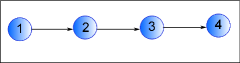
Figure 1: Linear graph $\mathrm{L}_{4}$ with 4 vertices.

According to MICMAC, for fixed $k<n$, vertex $j$ will only influence vertex $j+k$. Thus the vertices $\{1,...,n-k\}$ are the most influential ones each with influence $1$. For $k\geq n$ the matrix of indirect influences vanishes. For example MICMAC for $\mathrm{L}_{3}$ and $\mathrm{L}_{4}$, with $k=4$, predicts vanishing influences and dependencies.

PageRank for $\mathrm{L}_{3}$ gives the dependency vector $(0.17,0.34,0.47)$ making vertex $3$ the most dependent one. For $n=4$ PageRank dependencies are $(0.12,0.21,0.30,0.37)$. Again, we see that vertex $4$ is the most dependent one, and that vertex $1$ has a positive dependency. One can check that according to PageRank the dependency of vertex $1$ in the graph $\mathrm{L}_{n}$ is given by $0.17,\ 0.12,\ 0.08,\ 0.059,\ 0.046\$ as the parameter $n$ increases from $3$ to $7$. For large $n$ we expect PageRank to produce an almost vanishing dependency for vertex $1$; for small $n$ though this dependency is not quite zero and may be significative.

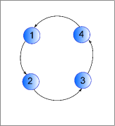
Figure 2: Cyclic graph with 4 vertices.

For $\mathrm{L}_{3}$ and $\lambda=0.5$, the Heat Kernet method gives the vectors $f=(0.98,0.9,0.6)$ and $d=(0.6,0.9,0.98).$ Notice that vertex $3$ has a non-vanishing influence, and vertex $1$ a non-vanishing influence. The highest influence and dependency of a vertex is on itself. Indeed, self-influence is responsible for more than half of the total influence of a vertex.

For $\mathrm{L}_{3}$ and $\lambda=1$, the PWP method gives the vectors $f=(1.5,1,0)$ and $d=(0,1,1.5).$ Vertex $3$ is the most dependent and has a vanishing influence; vertex $1$ has a vanishing dependency. For $\mathrm{L}_{4}$ and $\lambda=1,$ PWP yields the vectors $f=(\frac{5}{3},\frac{3}{2},1,0)$ and $d=(0,1,\frac{3}{2},\frac{5}{3}).$ Thus vertex $4$ is the most dependent one and has vanishing influence; vertex $1$ has a vanishing dependency and has the highest influence.

For arbitrary $n$ and $\lambda$ one can check that PWP yields the matrix $T$ given by

$$T_{j+s,j}=\left\{\begin{array}[]{cc}\frac{\lambda^{s}}{e_{+}^{\lambda}s!}&\mbox{ for \ }1\leq j<n,\ \ \ 1\leq s\leq n-j\\ 0&\mbox{otherwise.}\end{array}\right.$$

From the expression above we see that for $s\leq n-j-1$ we have

$$\frac{T_{j+s+1,j}}{T_{j+s,j}}=\frac{\lambda}{s+1},$$

and therefore we obtain that

$$T_{j+s+1,j}>T_{j+s,j}\ \ \ \ \ \ \mbox{for}\ \ \ \ s<\lambda-1,$$

$$T_{j+s+1,j}<T_{j+s,j}\ \ \ \ \ \ \mbox{for}\ \ \ \ s>\lambda-1.$$

Therefore $T_{j+s,j}$ achieves its maximum, for fixed $j$, at $s=\lfloor\lambda\rfloor$ if $\lambda\geq 1$, and at $s=1$ if $\lambda<1$.

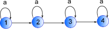
Figure 3: Jordan graph with 4 vertices.

Example 5.

Let $\mathrm{C}_{n}$ be the cyclic graph on $[n]$, i.e. the graph with an edge from $j$ to $j+1$ for $j<n$ and an edge from $n$ to $1$. Figure 2 shows the cyclic graph $\mathrm{C}_{4}$. In this case the four methods yield the same vector of dependencies, but they do so for quite different reasons.

MICMAC makes the influence and dependence of each vertex equal to $1$. Indeed for fixed $k$, vertex $j$ will only influence the vertex $j+k$ mod $n$.

The PageRank vector of dependencies is also $(1,....,1)$, indeed each vertex is equally dependent on every other vertex, i.e. the PageRank matrix $T$ has all its entries equal to $\frac{1}{n}.$

The Heat Kernel, for $n=4$ and $\lambda=0.5$, yield the vector of dependencies $(1,1,1,1)$. The influence of a vertex on the other vertices decreases as the distance in the cyclic ordering increases. The highest influence of a vertex is on itself.

With PWP the matrix $T$ of indirect influences is given, for $j,s\in[n]$ and $j+s$ taken mod $n$, by

$$T_{j+s,j}=\frac{1}{e_{+}^{\lambda}}\sum_{k=0}^{\infty}\frac{\lambda^{nk+s}}{(nk+s)!}.$$

Thus for $\lambda=1$ we have that

$$T_{j+s,j}=\frac{1}{e_{+}^{1}}\sum_{k=0}^{\infty}\frac{1}{(nk+s)!},$$

and therefore we get that

$$T_{j+1,j}>T_{j+2,j}>....>T_{j+n,j}=T_{j,j}.$$

Thus, the influence and the dependence of a vertex $j$ are both equal to $1$. Vertex $j$ influences all other vertices; it has a higher influence over the vertices closer to it in the cyclic ordering. Its lowest influence is on itself.

Example 6.

From Theorem 1, properties 2 and 3, choosing an appropriated basis one can always reduced the computation of the PWP matrix $T=T(D)$ of indirect influences to the case where $D$ is a Jordan block of a matrix in Jordan canonical form. We let $J_{n}(a)$ be the Jordan graph associated with a Jordan block with value $a$ on the diagonal. The Jordan graph $\mathrm{J}_{4}$ is shown in Figure 3.

Thus, we assume that $D$ is a matrix such that $D_{jj}=a,\ D_{j+1,j}=1,\ \mbox{and}\ D_{ij}=0\ \mbox{otherwise.}$ Vertex $j$ exerts a non-vanishing indirect influence over the vertices $j+s$ with $0\leq s\leq n-j.$ Notice that at vertex $j$ a path can either stay at $j$ or move to $j+1$, thus the MICMAC matrix for fixed $k$ is given by

$$|P_{k}(j+s,j)|={k\choose s}a^{k-s}.$$

Therefore the PWP matrix $T$ of indirect influences is given by

$$T_{j+s,s}=\frac{1}{e_{+}^{\lambda}}\sum_{k=s}^{\infty}{k\choose s}a^{k-s}\frac{\lambda^{k}}{k!}=\frac{e^{a\lambda}\lambda^{s}}{(e^{\lambda}-1)s!}.$$

Example 7.

Consider the star graph $\mathrm{S}_{n}$ with vertex set $\{0,1,....,n\}$, see Figure 4, and directed edges from $0$ to $i\in[n]$ and viceversa. It is not hard to see that the PWP matrix of indirect influences $T$ is a symmetric matrix given, for $i,j\in[n],$ by

$$T_{0,0} = \frac{e^{\lambda\sqrt{n}}+e^{-\lambda\sqrt{n}}}{2e_{+}^{\lambda}},$$

$$T_{j,0} = \frac{1}{e_{+}^{\lambda}}\sum_{k=0}^{\infty}n^{k}\frac{\lambda^{2k+1}}{(2k+1)!},$$

$$T_{i,j} = \frac{e^{\lambda\sqrt{n}}+e^{-\lambda\sqrt{n}}}{2ne_{+}^{\lambda}}.$$

Thus the vertex with greater influence and dependence is the vertex $0$. PageRank yields a similar result making $0$ the most dependent vertex.

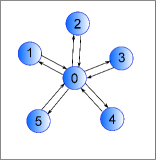
Figure 4: Star graph with 6 vertices.

7 Final comments

The main goal of this note is to propose an alternative method for counting indirect influences. It seems convenient to have a pool of options, as well as a comparative study of the various possibilities. We introduced the PWP method for counting indirect influences. Applications of PWP to real-world networks is currently underway. We worked with a discrete scenario where influences are transmitted linearly. Lifting those restrictions will conduce to continuous non-linear models. This more general setting will be considered elsewhere.

ragadiaz@gmail.com
Escuela de Matemáticas, Universidad Sergio Arboleda, Bogotá, Colombia

References

- [1] H. Blandín, R. Díaz, Rational combinatorics, Adv. in Appl. Math. 40 (2008) 107-126.
- [2] S. Brin, R. Motwani, L. Page, T. Winograd, The PageRank citation ranking: Bringing order to the web, Technical Report, Stanford Digital Library Technologies Project, 1998.
- [3] F. Chung, The heat kernel as the pagerank of a graph, Proc. Natl. Acad. Sci. U. S. A. 104 (2007) 19735-19740.
- [4] R. Díaz, E. Pariguan, Super, Quantum and Non-Commutative Species, Afr. Diaspora J. Math. 8 (2009) 90-130.
- [5] M. Godet, De l’Anticipation l’Action, Dunod, París 1992.
- [6] A. Langville, C. Meyer, Deeper Inside PageRank, Internet Mathematics 1 (2004) 335-400.