Recent Progress in Jet Algorithms and Their Impact in Underlying Event Studies

Abstract

Recent developments in jet clustering are reviewed. We present a list of fast and infrared and collinear safe algorithms, and also describe new tools like jet areas. We show how these techniques can be applied to the study of underlying event or, more generally, of any background which can be considered distributed in a sufficiently uniform way.

1 Recent Developments in Jet Clustering

The final state of a high energy hadronic collision is inherently extremely complicated. Hundreds or even thousands of particles will be recorded by detectors at the Large Hadron Collider (LHC), making the task of reconstructing the original (simpler) hard event very difficult. This large number of particles is the product of a number of branchings and decays which follow the initial production of a handful of partons. Usually only a limited number of stages of this production process can be meaningfully described in quantitative terms, for instance by perturbation theory in QCD. This is why, in order to compare theory and data, the latter must first be simplified down to the level described by the theory.

Jet clustering algorithms offer precisely this possibility of creating calculable observables from many final-state particles. This is done by clustering them into jets via a well specified algorithm, which usually contains one or more parameters, the most important of them being a “radius” $R$ which controls the extension of the jet in the rapidity-azimuth plane. One can also choose a recombination scheme, which controls how partons’ (or jets’) four-momenta are combined. The choice of a jet algorithm, its parameters and the recombination scheme is called a jet definition [1], and must be specified in full (together with the initial particles sample) in order for the process

$$\left\{\mathrm{particles}\right\}\stackrel{{\scriptstyle\mathrm{jet~{}definition}}}{{\longrightarrow}}\left\{\mathrm{jets}\right\}$$ (1)

to be fully reproducible and the final jets to be the same.

While (almost) any jet definition can produce sensible observables, not all of them will produce one which is calculable in perturbation theory. For this to be true, the jet algorithm must be infrared and collinear safe (IRC safe) [2], meaning that actions producing configurations that lead to divergences in perturbation theory, namely the emission of a very soft particle or a collinear splitting of a particle into two) must not produce any change in the jets returned by the algorithm.

The importance for jet algorithms to be IRC safe had been recognized as early as 1990 in the ‘Snowmass accord’ [3], together with the need for them to be easily applicable both on the theoretical and the experimental side. However, many of the implementations of jet clustering algorithms used in the following decade and a half failed to provide these characteristics: cone-type algorithms were typically infrared or collinear unsafe beyond the two or three particle level (see [1] for a review), whereas recombination-type algorithms were usually considered too slow to be usable at the experimental level in hadronic collisions.

This deadlock was finally broken by two papers, one in in 2005 [4], which made sequential recombination type clustering algorithms like $k_{t}$ [5, 6] and Cambridge/Aachen [7, 8] fast, and one in 2007, which introduced SISCone [9], a cone-type algorithm which is infrared and collinear safe. A third paper introduced, in 2008, the anti-$k_{t}$ algorithm [10], a fast, IRC safe recombination-type algorithm which however behaves, for many practical purposes, like a nearly-perfect cone. This set of algorithms (see Table 1), all available through the FastJet package [11], allows one to replace most of the unsafe algorithms still in use with fast and IRC safe ones, while retaining their main characteristics (for instance, the MidPoint and the ATLAS cone could be replaced by SISCone, and the CMS cone could be replaced by anti-$k_{t}$).

Jet algorithm	Type of algorithm, (distance measure)	algorithmic complexity
$k_{t}$ [5, 6]	SR, $d_{ij}=\min(k_{ti}^{2},k_{tj}^{2})\Delta R_{ij}^{2}/R^{2}$	$N\ln N$
Cambridge/Aachen [7, 8]	SR, $d_{ij}=\Delta R_{ij}^{2}/R^{2}$	$N\ln N$
anti-$k_{t}$ [10]	SR, $d_{ij}=\min(k_{ti}^{-2},k_{tj}^{-2})\Delta R_{ij}^{2}/R^{2}$	$N^{3/2}$
SISCone [9]	seedless iterative cone with split-merge	$N^{2}\ln N$

Table 1: List of some of the IRC safe algorithms available in FastJet. SR stands for ‘sequential recombination’. $k_{ti}$ is a transverse momentum, and the angular distance is given by $\Delta R_{ij}^{2}=\Delta y_{ij}^{2}+\Delta\phi_{ij}^{2}$.

2 Jet Areas

A by-product of the speed and the infrared safety of the new algorithms (or new implementations of older algorithms) was found to be the possibility to define in a practical way the area of a jet, which measures its susceptibility to be contaminated by a uniformly distributed background of soft particles in a given event.

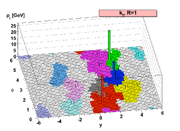
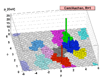
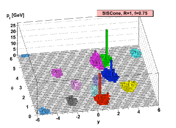
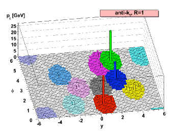
Figure 1: Typical jet outlines returned by four different IRC safe jet clustering algorithms. From[10].

In their most modest incarnation, jet areas can be used to visualize the outline of the jets returned by an algorithm so as to appreciate, for instance, if it returns regular (“conical”) jets or rather ragged ones. An example is given in Fig. 1.

Jet areas are amenable, to some extent, to analytic treatments [12], or can be measured numerically with the tools provided by FastJet. These analyses disprove the common assumption that all cone-type algorithms have areas equal to $\pi R^{2}$. In fact, depending on exactly which type of cone algorithm one considers, its areas can differ, even substantially so, from this naive estimate: for instance, the area of a SISCone jet made of a single hard particle immersed in a background of many soft particles is $\pi R^{2}/4$ (this little catchment area can explain why other iterative cone algorithms with a split-merge step, like the MidPoint algorithm in use at CDF, have often been seen to fare ‘well’ in noisy environments). One can analyse next the $k_{t}$ and the Cambridge/Aachen algorithms, and see that their single-hard-particle areas turn out to be roughly $0.81\pi R^{2}$. Finally, this area for the anti-$k_{t}$ algorithm is instead exactly $\pi R^{2}$. This fact, together with its regular contours shown in Fig. 1, explains why it is usually considered to behave like a ‘perfect cone’.

Jet areas also allow one to use some jet algorithms as tools to measure the level of a sufficiently uniform background which accompanies harder events. This can be accomplished by following the procedure outlined in [13]: for each event, all particles are clustered into jets using either the $k_{t}$ or the Cambridge/Aachen algorithms, and the transverse momentum $p_{t,j}$ and the area $A_{j}$ of each jet are calculated. One observes that a few hard jets have large values of transverse momentum divided by area, whereas most of the other, softer jets have smaller (and similar) values of this ratio. The background level $\rho$, transverse momentum per unit area in the rapidity-azimuth plane, is then obtained as

$$\rho=\mathrm{median}\left\{\frac{p_{t,j}}{A_{j}}\right\}_{j\in{\cal R}}\,.$$ (2)

The range ${\cal R}$ should be the largest possible region of the rapidity-azimuth plane over which the background is expected to be constant.

The operation of taking the median of the $\{p_{t,j}/A_{j}\}$ distribution is, to some extent, arbitrary. It has been found to give sensible results, provided that the range ${\cal R}$ contains sufficiently many soft background jets – at least about ten (twenty) of them, if only one (two) harder jets are also present in ${\cal R}$, are usually enough [14].

3 Underlying Event Studies

To a certain extent, and within certain limits, the background to a hard collision created by the soft particles of the underlying event (EU) can be considered fairly uniform. It becomes then amenable to be studied with the technique introduced in the previous Section. This constitutes an alternative to the usual and widespread approach (see for instance [15, 16]) of triggering on a leading jet, and selecting the two regions in the azimuth space which are transverse to its direction and to that of the recoil jet. These two regions are considered to be little affected by hard radiation (in the least energetic of them it is expected to be suppressed by at least two powers of $\alpha_{s}$), and therefore one can expect to be able to measure the UE level there.

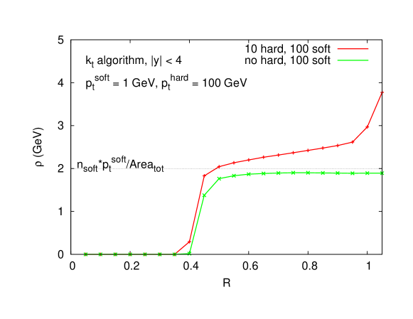
Figure 2: Determination of the background level $\rho$ of a toy-model random underlying event, as a function of the radius parameter $R$. Each point is the result of averaging over many different realizations. The parameters have been adjusted to roughly reproduce the situation expected at the LHC.

This way of selecting the UE can be considered a topological one: particles (or jets) are classified as belonging to the UE or not as a result of their position. On the other hand, the median procedure described in the previous Section can be thought of as a dynamical selection: no a priori hypotheses are made and, in a way that changes from one event to another, a jet is automatically classified as belonging to the hard event or to the background as a result of its characteristics (namely the value of the $p_{t,j}/A_{j}$ ratio). One can further show that this selection pushes the possible contamination from perturbative radiation to very large powers of $\alpha_{s}$: for a range ${\cal R}$ defined by $|y|<y_{max}$, perturbative contamination will only start at order $n\simeq 3y_{max}/R^{2}$ [13]. This gives $n\sim 24$ for $y_{max}=2$ and $R=0.5$, suggesting that the perturbative contribution is minimal.

A sensible criticism of this procedure is that the UE distribution is not necessarily uniform, and may for instance vary as a function of rapidity. A way around this is then to choose smaller ranges, located at different rapidity values, and repeat the $\rho$ determination in each of them. Of course care will have to be taken that the chosen ranges remain large enough to satisfy the criterion on the number of soft jets versus hard ones given in the previous Section: for instance, a range one unit of rapidity large can be expected to contain roughly $2\pi/(0.55\pi R^{2})\sim 15$ soft jets for $R=0.5$, which makes it marginally apt to the task.

A final word should be spent on which values of the radius parameter $R$ can be considered appropriate for this analysis. Roughly speaking, $R$ should be large enough for the number of ‘real’ jets (i.e. containing real particles) to be at last larger than the number of ‘empty jets’ (regions of the rapidity-azimuth plane void of particles, and not occupied by any ‘real’ jet). It should also be small enough to avoid having too many jets containing too many hard particles. Analytical estimates [13] and empirical evidence show that for UE estimation in typical LHC conditions one can expect values of the order of 0.5 – 0.6 to be appropriate. Much smaller values will return $\rho\simeq 0$, while larger values will tend to return progressively larger values of $\rho$, as a result of the increasing contamination from the hard jets. Fig. 2 shows results obtained with a toy model where 100 soft particles with $p_{T}^{soft}\simeq 1$ GeV are generated in a $|y|<4$ region. Ten hard particles, with $p_{T}^{hard}\simeq 100$ GeV, can be additionally generated in the same region. One observes how, after a threshold value for $R$, $\rho$ is estimated correctly for the soft-only case, while when hard particles are present they increasingly contaminate the estimate of the background.

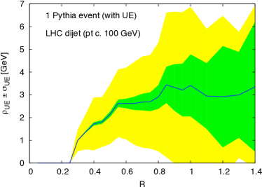
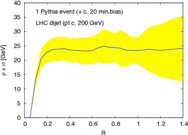
Figure 3: Determination of the background level $\rho$ in realistic dijet events at the LHC, with (right) and without (left) pileup. Preliminary results.

The same analysis can be performed on more realistic events, generated by Monte Carlo simulations. Fig. 3 shows the determination of $\rho$ in a simulated dijet event at the LHC, with and without pileup. In both cases the general structure of the toy-model in Fig. 2 can be seen, though it is worth noting that in the UE case (left plot) the slope can vary significantly from event to event, and also according to the Monte Carlo tune used [14]. The larger particle density (and probably higher uniformity) of the pileup case allows for an easier and more stable determination.

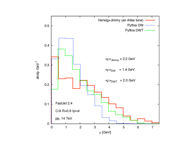
Figure 4: Distributions of $\rho$ from the UE over many simulated LHC dijet events ($p_{T}>50$ GeV, $|y|<4$), using different Monte Carlos and different UE tunes. Preliminary results.

Once a procedure for determining $\rho$ is available, one can think of many different applications. One possibility is of course to tune Monte Carlo models to real data by comparing rho distributions, correlations, etc. A preliminary example is given in fig. 4, where studying the distribution of $\rho$ can be seen to allow one to discriminate between UE models which would otherwise give similar values for the average contribution $\langle\rho\rangle$. More extensive studies are in progress [14].

Yet another use of measured $\rho$ values is the subtraction of the background from the transverse momentum of hard jets. Ref. [13] proposed to correct the four-momentum $p_{\mu j}$ of the jet $j$ by an amount proportional to $\rho$ and to the area of the jet itself (the susceptibility of the jet to contamination):

$$p_{\mu j}^{sub}=p_{\mu j}-\rho A_{\mu j}$$ (3)

where $A_{\mu j}$ is a four-dimensional generalization of the concept of jet area, normalized in such a way that its transverse component coincides, for small jets, with the scalar area $A_{j}$ [12]. One can show [13, 17] that such subtraction of the underlying event can improve in a non-negligible way the reconstruction of mass peaks even at very large energy scales. A similar procedure is also being considered [18] for heavy ion collisions, where the background can contribute a huge contamination, even larger than the transverse momentum of the hard jet itself (partly because of this, one usually speaks of ‘jet reconstruction’ in this context, rather than just ‘subtraction’). Initial versions of this technique have already been employed at the experimental level by the STAR Collaboration at RHIC in [19, 20], where IRC safe jets have been reconstructed for the first time in heavy ion collisions.

4 Conclusions

Since 2005 numerous developments have intervened in jet physics. A number of fast and infrared and collinear safe algorithms are now available, allowing for great flexibility in analyses. Tools have been developed and practically implemented to calculate jet areas, and these can used to study various types of backgrounds (underlying event, pileup, heavy ions background) and also to subtract their contribution to large transverse-momentum jets.

These new algorithms and methods (as well as the ones not mentioned in this talk, like the many approaches to jet substructure, see e.g. [21, 22, 23, 24, 25], useful in a number of new-physics searches) are transforming jet physics from being just a procedure to obtain calculable observables to providing a full array of precision tools with which to probe efficiently the complex final states of high energy collisions.

References

- [1] C. Buttar et al. (2008). 0803.0678 [hep-ph]
- [2] G. Sterman and S. Weinberg, Phys. Rev. Lett. 39, 1436 (1977)
- [3] J. E. Huth et al. Presented at Summer Study on High Energy Physics, Reaearch Directions for the Decade, Snowmass, CO, Jun 25 - Jul 13, 1990
- [4] M. Cacciari and G. P. Salam, Phys. Lett. B641, 57 (2006). hep-ph/0512210
- [5] S. Catani, Y. L. Dokshitzer, M. H. Seymour, and B. R. Webber, Nucl. Phys. B406, 187 (1993)
- [6] S. D. Ellis and D. E. Soper, Phys. Rev. D48, 3160 (1993). hep-ph/9305266
- [7] Y. L. Dokshitzer, G. D. Leder, S. Moretti, and B. R. Webber, JHEP 08, 001 (1997). hep-ph/9707323
- [8] M. Wobisch and T. Wengler (1998). hep-ph/9907280
- [9] G. P. Salam and G. Soyez, JHEP 05, 086 (2007). 0704.0292 [hep-ph]
- [10] M. Cacciari, G. P. Salam, and G. Soyez, JHEP 04, 063 (2008). 0802.1189
- [11] M. Cacciari, G. P. Salam, and G. Soyez, http://www.fastjet.fr/
- [12] M. Cacciari, G. P. Salam, and G. Soyez, JHEP 04, 005 (2008). 0802.1188
- [13] M. Cacciari and G. P. Salam, Phys. Lett. B659, 119 (2008). 0707.1378
- [14] M. Cacciari, G. P. Salam, and S. Sapeta, in preparation
- [15] CDF Collaboration, D. E. Acosta et al., Phys. Rev. D70, 072002 (2004). hep-ex/0404004
- [16] D. Acosta et al. CERN-CMS-NOTE-2006-067
- [17] M. Cacciari, J. Rojo, G. P. Salam, and G. Soyez, JHEP 12, 032 (2008). 0810.1304
- [18] M. Cacciari, J. Rojo, G. P. Salam, and G. Soyez, in preparation
- [19] STAR Collaboration, S. Salur (2008). 0809.1609
- [20] STAR Collaboration, S. Salur (2008). 0810.0500
- [21] J. M. Butterworth, A. R. Davison, M. Rubin, and G. P. Salam, Phys. Rev. Lett. 100, 242001 (2008). 0802.2470
- [22] J. Thaler and L.-T. Wang, JHEP 07, 092 (2008). 0806.0023
- [23] D. E. Kaplan, K. Rehermann, M. D. Schwartz, and B. Tweedie, Phys. Rev. Lett. 101, 142001 (2008). 0806.0848
- [24] L. G. Almeida et al. (2008). 0807.0234
- [25] S. D. Ellis, C. K. Vermilion, and J. R. Walsh (2009). 0903.5081.