Tight-binding modeling and low-energy behavior
of the semi-Dirac point

Abstract

We develop a tight-binding model description of semi-Dirac electronic spectra, with highly anisotropic dispersion around point Fermi surfaces, recently discovered in electronic structure calculations of VO₂/TiO₂ nano-heterostructures. We contrast their spectral properties with the well known Dirac points on the honeycomb lattice relevant to graphene layers and the spectra of bands touching each other in zero-gap semiconductors. We also consider the lowest order dispersion around one of the semi-Dirac points and calculate the resulting electronic energy levels in an external magnetic field. We find that these systems support apparently similar electronic structures but diverse low-energy physics.

The ability to prepare graphene (single graphite sheets) graphene_nat05 has spurred the study of electronic behavior of this unique system, in which a pair of Dirac points occur at the edge of the Brillouin Zone antonio . Bands extend linearly (referred to as “massless Dirac”) both to lower and higher energy from point Fermi surfaces. This unusual behavior requires special symmetry and non-bonding bands. In bilayer graphene graphene_bilayer , the linearly dispersing bands become quadratic, while retaining many of the symmetry properties. Spin-orbit coupling in these systems should lead to a gapped insulator in the bulk. Gapless modes remain at the edge of the system, protected by topological properties and time-reversal symmetry. This new state of matter, insulating in the bulk and metallic at the edges, has been called a topological insulator qshe_graphene ; fu .

Point Fermi surfaces also arise in gapless semiconductors in which the bands extend quadratically (“massively”) from a single point separating valence and conduction bands Tsidilkovski . However, these systems are, generically, not topological insulators. It has been argued that in HgTe quantum wells, where $s$ and $p$ bands overlap each other at the $\Gamma$ point as a function of well thickness, Dirac-like spectra can also arise with exotic topological properties. Due to the enhanced spin-orbit coupling in these materials, a state of matter exhibiting quantum spin Hall effect, has been predicted bernevig and observed konig .

Recent developments in the synthesis of controlled nanostructures, heterojunctions and interfaces of transition metal oxides represent one of the most promising areas of research in materials physics. While several recent studies of oxide interfaces have focused on the polarity discontinuity that can give rise to unexpected states between insulating bulk oxides, including conductivity ohtomo ; hwang , magnetism magn_IF , orbital order pentcheva , even superconductivity IF_sc , unanticipated behavior unrelated to polarity can also arise. The VO₂/TiO₂ interface involves no polar discontinuity, but only an open-shell charge and local magnetic discontinuity, according to the change $d^{1}\leftrightarrow d^{0}$ across the interface.

It was recently discovered vo2_tio2 that a three unit cell slab of VO₂ confined within insulating TiO₂ possesses a unique band structure. It shows four symmetry related point Fermi surfaces along the (1,1) directions in the 2D Brillouin zone, in this respect appearing to be an analog to graphene. The dispersion away from this point is however different and unanticipated: a gap opens linearly along the symmetry line, but opens quadratically along the perpendicular direction. The descriptive picture is that the associated (electron or hole) quasiparticles are relativistic along the diagonal with an associated “speed of light” $v_{F}$, as they are in graphene in both directions, but they are non-relativistic in the perpendicular direction, with an effective mass $m$. Seemingly the laws of physics (energy vs. momentum) are different along the two principal axes. The situation is neither conventional zero-gap semiconductor-like, nor graphene-like, but has in some sense aspects of both. This kind of spectra was found to be robust under modest changes in the structure.

Here, we develop a tight-binding model description of this semi-Dirac spectra. We find that a three-band model is needed, which can be downfolded to two bands at low energies. A variant of the model, with only two bands, gives rise to anisotropic Dirac spectra, where one has linearly dispersing modes around point Fermi surfaces, with very different “speed of light” along two perpendicular axes. A common feature of the various systems discussed above are point Fermi-surfaces. From a device point of view, for example in thinking of p-n or p-n-p junctions, these systems may share common qualitative features. The actual dispersion, which would give rise to different density of states, may control more quantitative differences. However, a more fundamental difference may be in their topological properties.fu ; thouless ; haldane ; moore

We begin with a 3-band tight-binding model of spinless fermions [corresponding to the half-metallic VO₂ trilayer although the system could also be nonmagnetic (spin degenerate)], on a square-lattice, defined by the Hamiltonian

$${\cal H}= \sum_{\alpha=1}^{3}(\sum_{i}\epsilon_{\alpha}n_{i,\alpha}+\sum_{<i,j>}t_{\alpha}(c_{i,\alpha}^{\dagger}c_{j,\alpha}+h.c.))$$

$$+\lambda_{1}\sum_{<i>,\pm}(c_{i,1}^{\dagger}c_{i\pm\hat{x},3}-c_{i,1}^{\dagger}c_{i\pm\hat{y},3}+h.c.)$$

$$+\lambda_{2}\sum_{<i>,\pm}(c_{i,2}^{\dagger}c_{i\pm\hat{x},3}-c_{i,2}^{\dagger}c_{i\pm\hat{y},3}+h.c.)$$

with $\epsilon_{3}>>\epsilon_{1},\epsilon_{2}$, so that we have two overlapping bands $1$ and $2$, with no coupling between them. Instead, they couple through the third band, by a coupling which changes sign under rotation by $90$ degrees. Such a coupling can be shown to arise by symmetry between $d$ and $s$ orbitals, for example. The important aspect is that the coupling vanishes along the symmetry line, allowing the bands to cross (they have different symmetries along the (1,1) line). Now, since the third band is far from the Fermi energy it can be taken as dispersionless. Furthermore, without affecting any essential physics, we take $t_{1}=-t_{2}=t$ and $\lambda_{1}=\lambda_{2}=t^{\prime}$. Thus, in momentum space the Hamiltonian becomes a $3\times 3$ matrix:

$$H=\begin{pmatrix}\widetilde{\varepsilon}_{1k}&0&V_{k}\\ 0&\widetilde{\varepsilon}_{2k}&V_{k}\\ V_{k}&V_{k}&\varepsilon_{3}\end{pmatrix}$$ (2)

where the dispersions and coupling are given by

Using the fact that orbital 3 is distant in energy, the three-orbital problem can be downfolded to a renormalized two orbital problem which becomes (neglecting a parallel shift of the two remaining bands)

$$H=\begin{pmatrix}\widetilde{\varepsilon}_{1k}&\frac{V_{k}^{2}}{\varepsilon_{3}}\\ \frac{V_{k}^{2}}{\varepsilon_{3}}&\widetilde{\varepsilon}_{2k}\end{pmatrix}$$ (5)

The eigenvalues $E_{k\pm}$ of $H$ as given by

$$E_{k\pm}=\frac{\widetilde{\varepsilon}_{1k}+\widetilde{\varepsilon}_{2k}}{2}\pm\frac{1}{2}\sqrt{(\widetilde{\varepsilon}_{1k}-\widetilde{\varepsilon}_{2k})^{2}+4[{\frac{V_{k}^{2}}{\varepsilon_{3}}}]^{2}}$$ (6)

With some (not very stringent) restrictions on $\varepsilon_{1}-\varepsilon_{2}$ to ensure that the uncoupled bands actually overlap, the two bands touch only at the point $\vec{k}_{sd}$ along the (1,1) lines where $\widetilde{\varepsilon}_{1k}=\widetilde{\varepsilon}_{2k}$, otherwise the two bands lie on either side of the touching point (the Fermi energy). When the 2$\times$2 Hamiltonian is expanded around the semi-Dirac point $\vec{k}_{sd}$ it becomes

$$H=\begin{pmatrix}\widetilde{\varepsilon}_{1k}&\frac{V_{k}^{2}}{\varepsilon_{3}}\\ \frac{V_{k}^{2}}{\varepsilon_{3}}&\widetilde{\varepsilon}_{2k}\end{pmatrix}\rightarrow\begin{pmatrix}v_{F}q_{2}&q_{1}^{2}/2m\\ q_{1}^{2}/2m&-v_{F}q_{2}\end{pmatrix}$$ (7)

where $q_{2}$ and $q_{1}$ denote the distance from $\vec{k}_{sd}$ along the (1,1) symmetry direction, and the orthogonal (1,${\bar{1}}$), respectively. The Fermi velocity $v_{F}$ and effective mass $m$ can be related explicitly to the tight binding model parameters, and also calculated by standard ab initio techniques. The dispersion relation is that found for the three layer slab of VO₂ trilayer in TiO₂ at low energy,

$$E_{q\pm}\rightarrow\pm\sqrt{(q_{1}^{2}/2m)^{2}+(v_{F}q_{2})^{2}}.$$ (8)

For comparison, the graphene dispersion relation is $E^{g}_{q\pm}=\pm v_{F}\sqrt{q_{1}^{2}+q_{2}^{2}}$. A plot of the low-energy dispersion of the model giving rise to a semi-Dirac point in the 2D Brillouin Zone is shown in Fig. 1. For the VO₂ trilayer,vo2_tio2 this dispersion holds up to 10-30 meV in the valence and conduction bands.

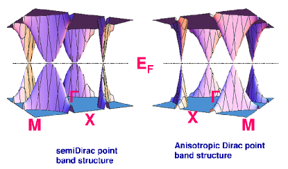
Figure 1: On the left, the plot shows the low energy band eigenvalues $E_{q\pm}$ in a region near $E_{F}$ for the semi-Dirac point. On the right is the same plot for the anisotropic Dirac point.

A few observations can be made at this point. First, if the original bands 1 and 2 were simply coupled by the same anisotropic mixing $V_{k}$ (without any third band in the picture), then anisotropic Dirac points (rather than semi-Dirac points) occur along the (1,1) directions. This dispersion is also shown in Fig. 1. This type of two-band situation should not be particularly unusual, hence Dirac points in 2D systems are probably not as unusual as supposed, i.e. they are not restricted to graphene nor are they restricted to high symmetry points.

While the constant energy surfaces of our model may appear to be elliptical (the common situation; the Dirac point has circular FSs), they are actually quite distinct. As $E\rightarrow$0 the velocity is constant in one direction and is $\sqrt{2mE}$ in the other; the FSs vanish as needles with their long axis perpendicular to the (1,1) direction. This can be seen in Fig. 2, showing the constant energy surfaces for electron doping according to our model, showing the 4 semi-Dirac points in the tetragonal k_x-k_y Brillouin zone. The density of states (DOS) n(E), which is constant for effective mass systems and goes as $|E|$ for graphene, is proportional to $\sqrt{|E|}$ at a semi-Dirac point. When doped, the density of carriers will follow $n(E_{F})\propto|E_{F}|^{3/2}$ behavior.

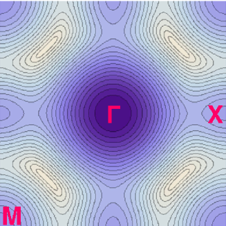
Figure 2: Plot showing the Fermi surfaces for electron doping that derive from the low energy excitation spectra of the semi-Dirac point at the $\Gamma-M$ direction in the k_x-k_y plane of the square Brillouin zone.

Another observation is that the same bands $E_{q\pm}$ can be obtained from related but distinct low-energy models, such as

$$H_{2}=\begin{pmatrix}v_{F}q_{2}&iq_{1}^{2}/2m\\ -iq_{1}^{2}/2m&-v_{F}q_{2}\end{pmatrix}$$ (9)

and

$$H_{3}=\begin{pmatrix}0&q_{1}^{2}/2m+iv_{F}q_{2}\\ q_{1}^{2}/2m-iv_{F}q_{2}&0\end{pmatrix}.$$ (10)

Although the bands resulting from $H_{2}$ and $H_{3}$ are the same, the eigenfunctions are different and are intrinsically complex for $H_{2}$ and $H_{3}$ unlike for the specific semi-Dirac point we discuss.

One of the issues of most interest to such systems is the behavior in a magnetic field. Making the usual substitution $\vec{q}\rightarrow\vec{p}+\frac{e}{c}\vec{A}$ with momentum operator $\vec{p}$ and vector potential $\vec{A}$, we find the Landau gauge $\vec{A}=B(-x_{2},0,0)$ to be the most convenient here. First, however, we note that the characteristics of the two directions, the mass $m$ and velocity $v_{F}$, introduce a natural unit of momentum $p_{o}=mv_{F}$ and length $x_{o}=\hbar/p_{o}$, and of energy $e_{o}=mv_{F}^{2}/2$. Introducing the atomic unit of magnetic field $B_{\circ}$ such that $\mu_{B}B_{\circ}$ = 1 Ha, and the dimensionless field $b=B/B_{\circ}$, units can be scaled away from the Hamiltonian by defining for each coordinate $x$

$$x_{2}=\Large(\frac{{1}}{\gamma b}\Large)^{2/3}x_{\circ}\tilde{x}_{2},$$ (11)

and similarly for $x_{1}$. Here $\gamma$ is the dimensionless ratio of the two natural energy scales: $\gamma=\mu_{B}B_{\circ}/(mv_{F}^{2}/2)$. Under this scaling

$$p_{1}+\frac{e}{c}A_{1}=p_{1}-\frac{e}{c}Bx_{2}\rightarrow p_{\circ}(\gamma b)^{2/3}(\tilde{p}_{1}-\tilde{x}_{2})$$ (12)

where $\tilde{p}_{1},\tilde{x}_{1}$ are conjugate dimensionless variables, etc. Thus all possible semi-Dirac points (all possible $m$ and $v_{F}$ combinations) scale to a single unique semi-Dirac point, with the materials parameters determining only the overall energy scale. There is no limiting case in which the semi-Dirac point becomes either a Dirac point or a conventional effective mass zero-gap semiconductor. For the case of trilayer VO₂, $\gamma$ does not differ greatly from unity vo2_tio2 .

Shifting $\tilde{x}_{2}$ to $u=\tilde{x}_{2}-\tilde{p}_{1}$, with conjugate dimensionless momentum $p$, the Hamiltonian in a field becomes

$$H = 2e_{o}~{}(\gamma b)^{2/3}~{}[p~{}\sigma_{z}+\frac{1}{2}u^{2}~{}\sigma_{x}]$$

$$\equiv 2e_{o}~{}(\gamma b)^{2/3}~{}h.$$

The energy scale is much larger than for conventional orbits though smaller than in graphene antonio , so the VO₂ trilayer may display an integer quantum Hall effect at elevated temperature as does graphene roomtempQHE .

A scalar equation for the eigenvalues can be obtained from $h^{2}$. Introducing the operator $Q=p+iu^{2}/2$, the eigenvalues of $h^{2}$ are $Q^{{\dagger}}Q$ and $QQ^{{\dagger}}$, giving the mathematical problem

$$Q^{{\dagger}}Q\phi_{n}(u)\equiv\Large(-\frac{d^{2}~{}}{du^{2}}+\frac{1}{4}u^{4}-u\Large)\phi_{n}(u)=\varepsilon_{n}^{2}\phi_{n}(u).$$ (14)

The equation for $QQ^{{\dagger}}$ has the opposite sign of the linear term, with identical eigenvalues and eigenfunctions related by inversion. Note that every eigenfunction of $h$ is also an eigenfunction of $h^{2}$, and that although the potential is negative in the interval (0,4^1/3), the eigenvalues $\varepsilon_{n}^{2}$ must be non-negative.

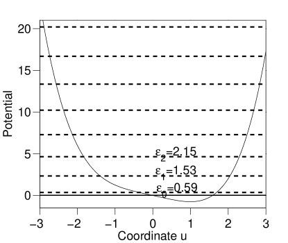
Figure 3: Potential energy function for the one-dimensional Schrödinger equation and the resulting quantized energy levels $\varepsilon_{n}^{2}$ of $h^{2}$. The lowest numerical vales of the three energy eigenvalues $\varepsilon_{n}=+\sqrt{\varepsilon_{n}^{2}}$ are provided.

We have obtained the eigenvalues both by precise numerical solution and by WKB approximation, finding that the latter is an excellent approximation. Initially neglecting the linear term in the potential, the WKB condition wkb

$$\int_{-\sqrt{2}\epsilon_{n}^{\frac{1}{2}}}^{\sqrt{2}\epsilon_{n}^{\frac{1}{2}}}\sqrt{\epsilon^{2}_{n}-\frac{1}{4}u^{4}}\ du=(n+\frac{1}{2})\pi$$ (15)

can be solved to give the WKB eigenvalues for the quartic potential as

$$\epsilon^{2}_{n}=\Large[3\sqrt{\frac{\pi}{2}}\frac{\Gamma(\frac{3}{4})}{\Gamma(\frac{1}{4})}\Large]^{4/3}(n+\frac{1}{2})^{\frac{4}{3}}=1.3765(n+\frac{1}{2})^{\frac{4}{3}}.$$ (16)

The linear perturbation corrects the eigenvalues only to second order, which is significant only for the ground state ($\sim$0.74 versus the numerical solution of 0.59). The WKB error is less than 0.01 for the first excited state and gets successively smaller for higher eigenvalues. We see then that the semi-Dirac system has eigenvalues in a magnetic field which scale as $B^{2/3}$ and increase as $(n+\frac{1}{2})^{2/3}$ as $n$ gets large. Both aspects lie between the behaviors for conventional Landau levels (linear in $B$, proportional the $n+\frac{1}{2}$) and the Dirac point behavior (proportional to $\sqrt{B~{}n}$), as might have been anticipated. Some low-lying eigenvalues of $h^{2}$ are shown in Fig. 3 against the potential well. Note that there is no zero-energy solution as in the graphene problem.

Another way in which Dirac spectra can arise on a square-lattice can be motivated in terms of the model of Bernevig et al. bernevig for HgTe quantum wells. In their model the two bands crossing each other have $s$ and $p$ characters respectively. Thus the interband hopping term changes sign under reflection. This can lead to a ($\sin{k_{x}}+i\sin{k_{y}}$) coupling between the bands. Note that in this model, only a single Dirac point can occur and it must be at $k=0$, when the two bands touch each other at that point. In contrast, in the models discussed here, there are four symmetry related semi-Dirac (or anisotropic Dirac) points whose location can vary continuously along the symmetry axis (1,1), with changes in band parameters. A feature unique (so far) to the VO₂ trilayer system is that point Fermi surface arises in a half metallic ferromagnetic system where time-reversal symmetry is broken. Applications of the VO₂ trilayer and related semi-Dirac point systems may provide unusual spintronics characteristics and applications.

In conclusion, we have developed a tight-binding model description of the semi-Dirac and anisotropic Dirac spectra relevant to VO₂-TiO₂ multi-layer systems. Our tight binding model contains nothing unconventional, indicating that semi-Dirac and anisotropic point systems are not as rare as has been assumed. The low energy characteristics of the semi-Dirac point are intermediate between those of zero-gap (massive) semiconductors and Dirac (massless) point systems. The study of such oxide nano-heterostructures has only just begun and they clearly promise a number of diverse electronic structures and novel phases of matter.

This project was supported by DOE grant DE-FG02-04ER46111 and by the Predictive Capability for Strongly Correlated Systems team of the Computational Materials Science Network. V.P. acknowledges financial support from Xunta de Galicia (Human Resources Program).

References

- (1) K.S. Novoselov et al., Nature 438, 197 (2005).
- (2) A. H. Castro Neto et al., Rev. Mod. Phys. 81, 109 (2009).
- (3) T. Ohta et al., Science 313, 5789 (2006).
- (4) C. L. Kane and E. J. Mele, Phys. Rev. Lett. 95, 226801 (2005).
- (5) L. Fu and C. L. Kane, Phys. Rev. B 76, 045302 (2007).
- (6) I. M. Tsidilkovski, Gapless Semiconductors (Akademie-Verlag Berlin, Berlin, 1988).
- (7) B. A. Bernevig et al., Science 314, 1757 (2006).
- (8) M. König et al., Science 318, 766 (2007).
- (9) A. Ohtomo et al., Nature 419, 378 (2002).
- (10) A. Ohtomo and H.Y. Hwang, Nature 423, 427 (2004).
- (11) A. Brinkman et al., Nat. Mater. 6, 493 (2007).
- (12) R. Pentcheva and W.E. Pickett, Phys. Rev. B 74, 035112 (2006).
- (13) N. Reyren et al., Science 317, 5842 (2007).
- (14) V. Pardo and W. E. Pickett, Phys. Rev. Lett. 102, 166803 (2009).
- (15) D. J. Thouless et al., Phys. Rev. Lett. 49, 405 (1982).
- (16) F. D. M. Haldane, Phys. Rev. Lett. 93, 206602 (2004).
- (17) J. E. Moore and L. Balents, Phys. Rev. B 75, 121306 (2007).
- (18) K. S. Novoselov et al., Science 315, 1379 (2007).
- (19) C. M. Bender and S. A. Orszag, Advanced Mathematical Methods for Scientists and Engineers (McGraw Hill, 1978), p. 523.