Discrete conformal variations and scalar curvature on piecewise flat two and three dimensional manifolds

1 Introduction

Consider a manifold constructed by identifying the boundaries of Euclidean triangles or Euclidean tetrahedra. When these form a closed topological manifold, we call such spaces piecewise flat manifolds (see Definition 1) as in [8]. Such spaces may be considered discrete analogues of Riemannian manifolds, in that their geometry can be described locally by a finite number of parameters, and the study of curvature on such spaces goes back at least to Regge [35]. In this paper, we give a definition of conformal variation of piecewise flat manifolds in order to study the curvature of such spaces.

Conformal variations of Riemannian manifolds have been well studied. While the most general variation formulas for curvature quantities is often complicated, the same formulas under conformal variations often take a simpler form. For this reason, it has even been suggested that an approach to finding Einstein manifolds would be to first optimize within a conformal class, finding a minimum of the Einstein-Hilbert functional within that conformal class, and then maximize across conformal classes to find a critical point of the functional in general [1]. Finding critical points of the Einstein-Hilbert functional within a conformal class is a well-studied problem dating back to Yamabe [48], and the proof that there exists a constant scalar curvature metric in every conformal class was completed by Trudinger [45], Aubin [2], and Schoen [40] (see also [27] for an overview of the Yamabe problem).

Implicitly, there has been much work on conformal parametrization of two-dimensional piecewise flat manifolds, many of which start with a circle packing on a region in $\mathbb{R}^{2}$ or a generalized circle packing on a manifold. Thurston found a variational proof of Andreev’s theorem ([44] [29]) and conjectured that the Riemann mapping theorem could be approximated by circle packing maps, which was soon proven to be true [39] (see also [43] for an overview of the theory). Another direction for conformal parametrization appears in [38], [28], and [42]. These and other works produce a rich theory of conformal geometries on surfaces and have led to many beautiful results about circle packings and their generalizations. The theory developed in this paper unifies several of these seemingly different notions of conformality to a more general notion. It also allows an explicit computation of variations of angles which allows one to glean geometric information. The geometric interpretation of the variations of angles was known in some instances (e.g., [23] [17]), but the proofs were explicit computations, which made them difficult to extend to more general cases. One of the main contributions of this paper is to show how these computations may be done in a more simple, geometric way which easily generalizes.

Existing literature on conformal parametrization of three-dimensional piecewise flat manifolds is much more sparse. A notion was given by Cooper and Rivin [12] which takes a sphere packing approach, and a rigidity result was produced (see also [37] and [18]). However, this theory requires that edge lengths come from a sphere packing, which is a major restriction of the geometry even on a single tetrahedron. In [17], the author was able to show by explicit computation that the variations of angles are related to certain areas and lengths of the piecewise flat manifold (in actuality, one needs the additional structure of a metric as described below). The theory developed in this paper generalizes this result to a general class of three dimensional piecewise flat manifolds. This generalization allows a geometric understanding of the variation of angles in a three-dimensional piecewise flat manifold under conformal variations, and the space of conformal variations is quite large and need not depend on the initial distribution of the edge lengths (unlike [17], where one must assume that the metric comes form a sphere packing structure).

The variation formulas for the curvature allow one to introduce a theory of functionals closely related to Riemannian functionals such as the Einstein-Hilbert functional. In two dimensions, many of these functionals are well studied, originally dating back to the work of Colin de Verdière [11]. In dimensions greater than three, the generalization of the Einstein-Hilbert functional was suggested by Regge [35] and has been well studied both in the physics and mathematics communities (see [22] for an overview). Recently, the functional was used to provide a constructive proof of Alexandrov’s theorem that a surface with positive curvature is the boundary of a polytope [4]. In this paper, we give a general construction for two-dimensional functionals arising from a conformal structure. We also consider variations of the Einstein-Hilbert-Regge functional with respect to conformal variations. Variation of this functional gives rise to notions of Ricci flat, Einstein, scalar zero, and constant scalar curvature metrics on piecewise flat manifolds. Our structure allows one to consider second variations of these functionals around fixed points, and give rigidity conditions near a Ricci flat or scalar zero manifold. An eventual goal is to prove theorems about the space of piecewise flat manifolds analogous to ones on Riemannian manifolds, for instance [26] [31].

Certain curvatures considered here have been shown to converge in measure to scalar curvature measure by Cheeger-Müller-Schrader in [8]. The proof in the general case does not appear to give the best convergence rate, and it is an open problem what this best convergence rate may be. It would be desirable to have a more precise control of the convergence and to prove a convergence of Ricci curvatures or of Einstein manifolds on piecewise flat spaces to Riemannian Einstein manifolds. Although the convergence result shows convergence to scalar curvature measure, it has been suggested that these curvatures are analogous to the curvature operator on a Riemannian manifold [7].

This paper is organized as follows. Section 2 gives definitions of geometric structures on piecewise flat manifolds in analogy to Riemannian manifolds and shows the main theorems on variations of curvature functionals. Section 3 derives formulas for conformal variations of angles. Section 4 translates these results to variations of curvatures and curvature functionals. Section 5 discusses some of the conformal structures already studied and shows how they fit into the framework developed here. Finally, Section 6 discusses discrete Laplacians, when they are negative semidefinite operators, and how this implies convexity results for curvature functionals and rigidity of certain metrics. The main theorems in the paper are Theorems 29 and 31 on the variations of angles, which could easily be applied to extend these results to the case of manifolds with boundary, Theorems 32 and 34 on the variation of curvature, which give analogues of the variation (11) of scalar curvature under conformal deformation of a Riemannian metric, Theorems 23 and 24 on the variation of curvature functionals, Theorems 40 and 41 on convexity of curvature functionals, and Theorems 43 and 44 on rigidity of zero scalar curvature and Ricci flat manifolds.

2 Geometric structures and curvature

2.1 Metric structure

We will consider certain analogues of Riemannian geometry. A Riemannian manifold $\left(M^{n},g\right)$ is a smooth manifold $M$ together with a symmetric, positive definite 2-tensor $g.$ A piecewise flat manifold is defined similarly to the definitions in [8].

Definition 1

A triangulated manifold $\left(M,T\right)$ is a topological manifold $M$ together with a triangulation $T$ of $M.$ A (triangulated) piecewise flat manifold $\left(M,T,\ell\right)$ is a triangulated manifold $\left(M,T\right)$ together with a function $\ell$ on the edges of the triangulation such that each simplex can be embedded in Euclidean space as a (nondegenerate) Euclidean simplex with edge lengths determined by $\ell$.

Nondegeneracy can be expressed by the fact that all simplices have positive volume. This condition can be realized as a function of the edge lengths using the Cayley-Menger determinant formula for volumes of Euclidean simplices.

In this paper we will consider only closed, triangulated manifolds although the definitions could be extended to more general spaces. We will describe simplices as $\left\{i,j,\ldots,k\right\},$ where $i,j,k$ are natural numbers. The length associated to an edge $\left\{i,j\right\}$ will be denoted $\ell_{ij},$ area associated to $\left\{i,j,k\right\}$ will be denoted $A_{ijk},$ and volume associated to $\left\{i,j,k,\ell\right\}$ will be denoted by $V_{ijk\ell}.$ Note that once lengths are assigned, area and volume can be computed using, for instance, the Cayley-Menger determinant formula. We will also use the notation $\gamma_{i,jk}$ to denote the angle at vertex $i$ in triangle $\left\{i,j,k\right\},$ and sometimes drop $jk$ when it is clear which triangle we are considering. A dihedral angle at edge $\left\{i,j\right\}$ in $\left\{i,j,k,\ell\right\}$ will be denoted $\beta_{ij,k\ell}$ and $k\ell$ will be dropped when it is clear which tetrahedron we are considering. In all of the following cases, the indices after the comma will be dropped when the context is clear.

Definition 2

Let $V\left(T\right)$ denote the vertices of $T,$ let $E\left(T\right)$ denote the edges of $T,$ and let $E_{+}\left(T\right)$ denote the directed edges in $T$ (there are two directed edges $\left(i,j\right)$ and $\left(j,i\right)$ associated to each edge $\left\{i,j\right\}$). For any of these vector spaces $X,$ let $X^{\ast}$ space of functions $h:X\rightarrow\mathbb{R}$.

Note that, for instance, if $d\in E_{+}\left(T\right)^{\ast}$ then $d=\sum_{\left(i,j\right)\in E_{+}}d\left(i,j\right)\phi_{ij}$, where $\phi_{ij}$ is the standard basis of $E_{+}\left(V\right)^{\ast}.$ We will use $d_{ij}$ (as in Definition 5) to denote either $d\left(i,j\right)$ or the function $d\left(i,j\right)\phi_{ij},$ and similarly with elements of $V\left(T\right)^{\ast}$ and $E\left(T\right)^{\ast}.$

Remark 3

We are implicitly assuming that the list of vertices determines the simplex uniquely. This is just to make the notation more transparent. We could also have indexed by simplices, such as $\ell_{\sigma^{2}},A_{\sigma^{3}},\gamma_{\sigma^{0}\subset\sigma^{3}},$ etc. This latter notation is much better if one wants to allow multiple simplices which share the same vertices.

Remark 4

A piecewise flat manifold is a geometric manifold, in the sense that it can be given a distance function in much the same way that a Riemannian manifold is given a distance function, i.e., by minimizing over lengths of curves.

The definition ensures that each simplex can be embedded isometrically in Euclidean space. The image of vertex $i$ in Euclidean space will be denoted $v_{i},$ the image of edge $\left\{i,j\right\}$ will be denoted $v_{i}v_{j},$ etc.

Piecewise flat manifolds are not exactly the analogue of a Riemannian manifold we will consider.

Definition 5

Let $\left(M,T\right)$ be a triangulated manifold. A piecewise flat pre-metric is an element $d\in E_{+}\left(T\right)^{\ast}$ such that $\left(M,T,\ell\right)$ is a piecewise flat manifold for the assignment $\ell_{ij}=d_{ij}+d_{ji}$ for every edge $\left\{i,j\right\}.$ A piecewise flat pre-metric $d$ is a metric if for every triangle $\left\{i,j,k\right\}$ in $T,$

$$d_{ij}^{2}+d_{jk}^{2}+d_{ki}^{2}=d_{ji}^{2}+d_{ik}^{2}+d_{kj}^{2}.$$ (1)

A piecewise flat, metrized manifold $\left(M,T,d\right)$ is a triangulated manifold $\left(M,T\right)$ with metric $d.$

For future use, we define the space of piecewise flat metrics on $\left(M,T\right).$

Definition 6

Define the space $\mathfrak{met}\left(M,T\right)$ to be

$$\mathfrak{met}\left(M,T\right)\mathfrak{=}\left\{d\in E_{+}\left(T\right)^{\ast}:\left(M,T,d\right)\text{ is a piecewise flat, metrized manifold}\right\}.$$

As shown in [19], condition (1) ensures that every simplex has a geometric center and a geometric dual which intersects the simplex orthogonally at the center. This dual is constructed from centers. Given a simplex embedded into space as $\left\{v_{1},v_{2},\ldots,v_{n}\right\},$ we have a center point to the simplex given by $c_{123\cdots n}.$ This point can be projected onto the $\left(n-1\right)$-dimensional simplices and successively projected onto all simplices, giving centers $c_{ij\cdots k}$ for all subsets of $\left\{1,2,\ldots,n\right\}.$ The centers can be constructed inductively by starting with centers of edges at a point $c_{ij}$ which is a (signed) distance $d_{ij}$ from vertex $i$ and $d_{ji}$ from vertex $j.$ Then one considers orthogonal lines through the centers, and condition (1) ensures that in each triangle, there is a single point where these three lines intersect, giving a center for the triangle. The construction may be continued for all dimensions, as described in [19].

For simplicity, let’s restrict to $n\leq 4.$ We will denote the signed distance between $c_{1234}$ and $c_{ijk}$ by $h_{ijk,\ell}$ and the signed distance between $c_{ijk}$ and $c_{ij}$ by $h_{ij,k}.$ The sign is gotten by the following convention. If $c_{1234}$ is on the same side of the plane defined by $v_{i}v_{j}v_{k}$ as the tetrahedron $v_{1}v_{2}v_{3}v_{4},$ then $h_{ijk,\ell}$ is positive, otherwise it is negative (or zero if the point is on that plane). Similarly, if $c_{ijk}$ is on the same side of the line defined by $v_{i}v_{j}$ as $v_{i}v_{j}v_{k}$ within that plane, then $h_{ij,k}$ is positive. Since it is clear that $h_{i,j}=d_{ij},$ we will not use the former. The side $v_{i}v_{j}$ is divided into a segment containing $v_{i}$ of length $d_{ij}$ and a segment containing $v_{j}$ of length $d_{ji}$ such that $\ell_{ij}=d_{ij}+d_{ji}.$ It is easy to deduce that $h_{ij,k}$ and $h_{ijk,\ell}$ can be computed by

$$h_{ij,k}=\frac{d_{ik}-d_{ij}\cos\gamma_{i,jk}}{\sin\gamma_{i,jk}}$$

and

$$h_{ijk,\ell}=\frac{h_{ij,\ell}-h_{ij,k}\cos\beta_{ij,k\ell}}{\sin\beta_{ij,k\ell}}.$$

See [19] or [4] for a proof. Importantly, these quantities work for negative values of the $d$’s and $h$’s. We will also consider the dual area $A_{ij,k\ell}$ of the edge $\left\{i,j\right\}$ in tetrahedron $\left\{i,j,k,\ell\right\},$ which is the signed area of the planar quadrilateral $c_{1234}c_{ijk}c_{ij}c_{ij\ell},$ where $i,j,k,\ell$ are distinct. The area is equal to

$$A_{ij,k\ell}=\frac{1}{2}\left(h_{ij,k}h_{ijk,\ell}+h_{ij,\ell}h_{ij\ell,k}\right).$$

These definitions of centers within a simplex induce a definition of geometric duals on a triangulation (see [19] for details). In particular, we will need the lengths or areas of duals of edges, defined in two and three dimensions as follows.

Definition 7

Let $\left(M^{2},T,d\right)$ be a piecewise flat, metrized manifold of dimension $2.$ Then edge $\left\{i,j\right\}$ is the boundary of two triangles, say $\left\{i,j,k\right\}$ and $\left\{i,j,\ell\right\}.$ The dual length $\ell_{ij}^{\ast}$ is defined as

$$\ell_{ij}^{\ast}=h_{ij,k}+h_{ij,\ell}.$$

Note that the two triangles can be embedded in the Euclidean plane together, and $\ell_{ij}^{\ast}$ is the signed distance between the centers of the two triangles.

Definition 8

Let $\left(M^{3},T,d\right)$ be a piecewise flat, metrized manifold of dimension $3.$ Then the dual length $\ell_{ij}^{\ast}$ (which is technically an area) is defined as

$$\ell_{ij}^{\ast} =\sum_{k,\ell}A_{ij,k\ell}$$

$$=\sum_{k,\ell}\frac{1}{2}\left(h_{ij,k}h_{ijk,\ell}+h_{ij,\ell}h_{ij\ell,k}\right),$$

where the sum is over all tetrahedra containing the edge $\left\{i,j\right\}.$

Notation 9

Most sums in this paper will be with respect to simplices, so a sum such as the one in Definition 8 means the sum over all tetrahedra $\left\{i,j,k,\ell\right\}$ containing the edge $\left\{i,j\right\},$ not the sum over all values of $k$ and $\ell$ (which would give twice the aforementioned sum).

The dual length is the area of a (generalized) polygon which intersects the edges orthogonally at their centers.

Remark 10

We specifically did not use the word Riemannian because it is not entirely clear what Riemannian should mean. Natural guesses would be that $d_{ij}>0$ for all directed edges $\left(i,j\right)$ or that all dual volumes are positive. However, we chose not to make such a distinction in this paper.

2.2 Curvature

In this section we define curvatures of piecewise flat metrized manifolds, many of which are the same as those for piecewise flat manifolds described by Regge [35] and Cheeger-Müller-Schrader [8]. Generally, curvature on a piecewise flat manifold of dimension $n$ is considered to be concentrated on codimension $2$ simplices, and the curvature at $\sigma$ is equal to the dihedral angle deficit from $2\pi$ multiplied by the volume of $\sigma,$ possibly with a normalization. Cheeger-Müller-Schrader [8] show that, under appropriate convergence of the triangulations, such a curvature converges in measure to scalar curvature measure $RdV.$ (In fact, Cheeger-Müller-Schrader prove a much more general result for all Lipschitz-Killing curvatures, but we will only consider scalar curvature.) We first define curvature for piecewise flat manifolds in dimension $2,$ which is concentrated at vertices.

Definition 11

Let $\left(M,T,\ell\right)$ be a two-dimensional piecewise flat manifold. Then the curvature $K_{i}$ at a vertex $i$ is equal to

$$K_{i}=2\pi-\sum_{j,k}\gamma_{i,jk},$$

where $\gamma_{i}$ are the interior angles of the triangles at vertex $i.$

Angles can be calculated from edge lengths using the law of cosines. Note that in two dimensions, curvature satisfies a discrete Gauss-Bonnet equation,

$$\sum_{i}K_{i}=2\pi\chi\left(M\right),$$

where $\chi$ is the Euler characteristic.

In dimension $3,$ the curvature is concentrated at edges.

Definition 12

Let $\left(M,T,\ell\right)$ be a three-dimensional piecewise flat manifold. Then the edge curvature $K_{ij}$ is

$$K_{ij}=\left(2\pi-\sum_{k,\ell}\beta_{ij,k\ell}\right)\ell_{ij}.$$

The dihedral angles can be computed as a function of edge lengths using the Euclidean cosine law to get the face angles, and then using the spherical cosine law to related the face angles to a dihedral angle.

There is an interpretation of $K_{ij}/\ell_{ij}$ in terms of deficits of parallel translations around the “bone” $\left\{i,j\right\}$. (See [35] for details.) For this reason, one may think of $K_{ij}/\ell_{ij}$ as some sort of analogue of sectional curvature or curvature operator (see [7]).

The fact that curvature is concentrated at edges often makes it difficult to compare curvatures with functions, which are naturally defined at vertices. For this reason, we will try move these curvatures to curvature functions based at vertices.

In the smooth case, the scalar curvature has interesting variation formulas. For instance, we may consider the Einstein-Hilbert functional,

$$\mathcal{EH}\left(M,g\right)=\int_{M}R_{g}dV_{g},$$

where $R_{g}$ is the scalar curvature and $dV_{g}$ is the Riemannian volume measure. Note that if $n=2,$ then the Gauss-Bonnet theorem says that $\mathcal{EH}\left(M,g\right)=2\pi\chi\left(M\right),$ but otherwise this functional is an interesting one geometrically. A well-known calculation (see, for instance, [3]) shows that if we consider variations of the Riemannian metric $\delta g=h$ on $M^{n},$ then

$$\delta\mathcal{EH}\left(M,g\right)\left[h\right]=\int_{M}g\left(E,h\right)dV,$$ (2)

where $E=R_{ij}-\frac{1}{2}Rg_{ij}$ is the Einstein tensor. It follows that critical points of this functional satisfy

$$R_{ij}-\frac{1}{2}Rg_{ij}=0.$$ (3)

Taking the trace of this equation with respect to the metric, we see that, if $n\neq 2$, this implies that

$$R_{ij}=0,$$ (4)

which is the Einstein or Ricci-flat equation. It also makes sense to consider either the constrained problem where volume is equal to one, or to consider the normalized functional

$$\frac{\mathcal{EH}\left(M^{n},g\right)}{\mathcal{V}\left(M^{n},g\right)^{\left(n-2\right)/n}},$$

where $\mathcal{V}$ is the volume. In both cases we find that critical points under a conformal variation correspond to metrics satisfying

$$R_{ij}=\lambda g_{ij}$$ (5)

for a constant $\lambda.$ Taking the trace and integrating, we see that

$$\lambda=\frac{1}{n}\frac{\mathcal{EH}\left(M^{n},g\right)}{\mathcal{V}\left(M^{n},g\right)}.$$ (6)

We now consider Regge’s analogue to the Einstein-Hilbert functional on three-dimensional piecewise flat manifolds.

Definition 13

If $\left(M^{3},T,\ell\right)$ is a three-dimensional piecewise flat manifold, the Einstein-Hilbert-Regge functional $\mathcal{EHR}$ is

$$\mathcal{EHR}\left(M,T,\ell\right)=\sum_{i,j}K_{ij},$$ (7)

where the sum is over all edges $\left\{i,j\right\}\in E\left(T\right).$

The analogue of the first variation formula (2) is

$$\frac{\partial}{\partial\ell_{ij}}\mathcal{EHR}\left(M,T,\ell\right)=2\pi-\sum_{k,\ell}\beta_{ij,k\ell}.$$ (8)

This was proven by Regge [35] and follows immediately from the Schläfli formula (see [30]). By analogy with the smooth case, we define the following.

Definition 14

A piecewise flat manifold $\left(M^{3},T,\ell\right)$ is Ricci flat if

$$K_{ij}=0$$

for all edges $\left\{i,j\right\}.$ It is Einstein with Einstein constant $\lambda\in\mathbb{R}$ if

$$K_{ij}=\lambda\ell_{ij}\frac{\partial\mathcal{V}}{\partial\ell_{ij}},$$ (9)

for all edges $\left\{i,j\right\},$ where

$$\mathcal{V}\left(M,T,\ell\right)\mathcal{=}\sum_{i,j,k,\ell}V_{ijk\ell}$$

is the total volume.

The term on the left of (9) can be made more explicit. Note that

$$3\mathcal{V}\left(M,T,\ell\right) =\left.\frac{d}{da}\right|_{a=1}a^{3}\mathcal{V}\left(M,T,\ell\right)$$

$$=\left.\frac{d}{da}\right|_{a=1}\mathcal{V}\left(M,T,a~{}\ell\right)$$

$$=\sum_{i,j}\ell_{ij}\frac{\partial\mathcal{V}}{\partial\ell_{ij}},$$

so

$$\lambda=\frac{\mathcal{EHR}\left(M,T,\ell\right)}{3\mathcal{V}\left(M,T,\ell\right)},$$

analogous to the smooth formula (6). Furthermore, we can explicitly compute for any tetrahedron $\left\{i,j,k,\ell\right\}$ that

$$\frac{\partial V_{ijk\ell}}{\partial\ell_{ij}}=\frac{1}{6}\ell_{ij}\ell_{k\ell}\cot\beta_{k\ell,ij}.$$ (10)

For brevity, we omit the proof of (10) since we will not use it. However, it can be proven by a direct computation of the derivatives of volume and of the dihedral angle.

As in the smooth case, studying the Einstein equation is quite difficult. Progress can be made by considering only certain variations of the metric. If one takes $\delta g=fg$ for a function $f,$ we have a conformal variation. Under conformal variations, the scalar curvature satisfies

$$\delta R\left[fg\right]=\left(1-n\right)\triangle f-Rf.$$ (11)

Since, under this variation, $\delta dV=\frac{n}{2}fdV,$ the variation of $\mathcal{EH}$ under a conformal variation is

$$\delta\mathcal{EH}\left(M,g\right)\left[fg\right] =\int\left[\left(1-n\right)\triangle f+\left(\frac{n}{2}-1\right)Rf\right]dV$$

$$=\left(\frac{n}{2}-1\right)\int RfdV.$$

In particular, $\left(\frac{n}{2}-1\right)R$ is the gradient of $\mathcal{EH}$ with respect to the $L_{2}\left(M,dV\right)$ inner product. We see that critical points of the functional under conformal variations correspond to when the scalar curvature is zero. Note that if we either (a) restrict to metrics with volume 1 or (b) normalize the functional, then we get constant scalar curvature metrics as critical points. The second variation of $\mathcal{EH}$ can be calculated from (11) to be

$$\delta^{2}\mathcal{EH}\left(M,g\right)\left[fg,fg\right] =\left(\frac{n}{2}-1\right)\int_{M}\left[\left(1-n\right)f\triangle f+\left(\frac{n}{2}-1\right)Rf^{2}\right]dV$$

$$=\left(\frac{n}{2}-1\right)\int_{M}\left[\left(n-1\right)\left|\nabla f\right|^{2}+\left(\frac{n}{2}-1\right)Rf^{2}\right]dV.$$

The second variation can be used to check to see if critical points are rigid, i.e., if there is a family of deformations of critical metrics.

The discrete formulation is motivated by the work of Cooper and Rivin [12], who looked at the sphere packing case. The goal is to formulate a conformal theory in the piecewise flat setting which allows simple variation formulas as in the smooth setting. First, we define the scalar curvature.

Definition 15

The scalar curvature $K$ of a three-dimensional piecewise flat, metrized manifold $\left(M^{3},T,d\right)$ is the function on the vertices defined by

$$K_{i}=\sum_{j}\left(2\pi-\sum_{k,\ell}\beta_{ij,k\ell}\right)d_{ij}.$$

This definition is much more general than the one in [12], but restricts to almost the same definition in the case of sphere packing (see Section 5 for the details). This curvature is in many ways analogous to the scalar curvature measure $RdV$ on a Riemannian manifold. Note that, unlike the edge curvatures $K_{ij},$ this curvature depends on the metric, not only the piecewise flat manifold. We also note the following important fact.

Proposition 16

If $\left(M^{3},T,d\right)$ is a three-dimensional piecewise flat, metrized manifold, then the Einstein-Hilbert-Regge functional can be written

$$\mathcal{EHR}\left(M,T,\ell\left(d\right)\right)=\sum_{i}K_{i}.$$

Proof. Simply do the sum and recall that $d_{ij}+d_{ji}=\ell_{ij}.$   

Now let us define conformal structure. The motivation for the definition will be seen in Theorems 23 and 24, and we will see some examples in Section 5. The reader may want to recall Definition 6.

Definition 17

A conformal structure $\mathcal{C}\left(M,T,U\right)$ on a triangulated manifold $\left(M,T\right)$ on an open set $U\subset V\left(T\right)^{\ast}$ is a smooth map

$$\mathcal{C}\left(M,T,U\right):U\rightarrow\mathfrak{met}\left(M,T\right)$$

such that if $d=\mathcal{C}\left(M,T,U\right)\left[f\right]$ then for each $\left(i,j\right)\in E_{+}$ and $k\in V$,

$$\frac{\partial\ell_{ij}}{\partial f_{i}}=d_{ij}$$

and

$$\frac{\partial d_{ij}}{\partial f_{k}}=0$$

if $k\neq i$ and $k\neq j$.

Notation 18

Often we will suppress the $U$ and simply refer to the domain of the conformal structure $\mathcal{C}\left(M,T\right).$

We can also define a conformal variation.

Definition 19

A conformal variation of a piecewise flat, metrized manifold $\left(M,T,\bar{d}\right)$ is a smooth curve $f:\left(-\varepsilon,\varepsilon\right)\rightarrow V\left(T\right)^{\ast}$ such that there exists a conformal structure $\mathcal{C}\left(M,T,U\right)$ with $f\left(-\varepsilon,\varepsilon\right)\subset U$ and $f\left(0\right)=\bar{d}.$ We call such a conformal structure an extension of the conformal variation.

An important point is that if we have a conformal structure or conformal variation, quantities such as $\frac{\partial\ell_{ij}}{\partial f_{j}}$ make sense. We will usually try to make statements in terms of $\frac{df_{i}}{dt}$ in order to reveal the appearance of discrete Laplacians, however sometimes it will be more convenient to express terms as partial derivatives. We note that a conformal variation is essentially independent of the extension in the following sense.

Proposition 20

Under a conformal variation $f\left(t\right)$ of $\left(M,T,\bar{d}\right)$, we have at $t=0$ that

$$\frac{d}{dt}\ell_{ij}=\bar{d}_{ij}\frac{df_{i}}{dt}+\bar{d}_{ji}\frac{df_{j}}{dt}.$$

In particular, at $t=0,$ for a given $\frac{df}{dt}\left(0\right),$ the variation of the length is independent of the extension.

Proof. From the definition of conformal structure, we have

$$\frac{d}{dt}\ell_{ij} =\frac{\partial\ell_{ij}}{\partial f_{i}}\frac{df_{i}}{dt}+\frac{\partial\ell_{ij}}{\partial f_{j}}\frac{df_{j}}{dt}$$

$$=d_{ij}\frac{df_{i}}{dt}+d_{ji}\frac{df_{j}}{dt}.$$

 

Notation 21

In the sequel, when we suppose a conformal variation, it will be understood that quantities such as $\frac{df_{i}}{dt}$ are evaluated at $t=0,$ though not stated.

There are often more than one extension to a conformal variation. For instance, for a triangle $\left\{1,2,3\right\},$ we may extend the metric defined by $d_{ij}=\frac{1}{2}$ for all $\left(i,j\right)\in E_{+}$ to several families where $f_{i}\left(t\right)=tx_{i},$ such as

$$d_{ij}\left(t\right)=\frac{1}{2}\exp\left(tx_{i}\right),$$

which corresponds to a circle packing conformal structure (see Section 5.1), and

$$d_{ij}\left(t\right)=\frac{1}{2}\exp\left(\frac{t}{2}\left(x_{i}+x_{j}\right)\right),$$

which corresponds to a perpendicular bisector conformal structure (see Section 5.3).

Remark 22

Often a conformal structure will be generated from a base metric, much the same way a conformal class on a Riemannian manifolds can be described as the equivalence class of metrics $e^{f}g_{0},$ where $f$ is a function on the manifold and $g_{0}$ is the base Riemannian metric. However, we have not defined it thus and, in general, one must be careful how the structures are defined if one wishes to partition all piecewise flat manifolds into conformal classes. We do not attempt this here, though there is a straightforward way to do this for perpendicular bisector conformal structures seen in Section 5.3.

In two dimensions, the fact that curvatures arise from conformal variations of a functional is not obvious, but can be proven.

Theorem 23

Fix a conformal structure $\mathcal{C}\left(M^{2},T,U\right)$ on a two dimensional triangulated manifold and suppose that $U$ is simply connected. Then there is a functional $F:U\rightarrow\mathbb{R}$ such that

$$\frac{\partial F}{\partial f_{i}}=K_{i}$$

for each $i\in V\left(T\right).$ Furthermore, the second variation of the functional under a conformal variation $f\left(t\right)$ can be expressed as

$$\frac{d^{2}F}{dt^{2}}=\frac{1}{2}\sum_{i,j}\frac{\ell_{ij}^{\ast}}{\ell_{ij}}\left(\frac{df_{j}}{dt}-\frac{df_{i}}{dt}\right)^{2}+K_{i}\frac{d^{2}f_{i}}{dt^{2}}.$$ (12)

This sort of formulation of the prescribed curvature problem in a variational framework has been studied by many people. See, for instance, [13] [36] [11] [9] [5] [41] [21]. However, no source to date has unified the theorem in the way of Theorem 23.

In three dimensions, the Einstein-Hilbert-Regge functional is a natural one to consider.

Theorem 24

For any conformal variation $f\left(t\right)$ of a three dimensional, piecewise flat, metrized manifold $\left(M,T,\bar{d}\right),$ we have,

$$\frac{d}{dt}\mathcal{EHR}\left(M,T,\ell\left(f\left(t\right)\right)\right) =\sum_{i}K_{i}\frac{df_{i}}{dt}$$ (13)

$$\frac{d^{2}}{dt^{2}}\mathcal{EHR}\left(M,T,\ell\left(f\left(t\right)\right)\right) =\sum_{i}\sum_{j\neq i}\left(\frac{\ell_{ij}^{\ast}}{\ell_{ij}}-\frac{q_{ij}}{2\ell_{ij}}K_{ij}\right)\left(\frac{df_{j}}{dt}-\frac{df_{i}}{dt}\right)^{2}$$ (14)

$$\;\;\;\;\;\;\;+\sum_{i}K_{i}\left[\left(\frac{df_{i}}{dt}\right)^{2}+\frac{d^{2}f_{i}}{dt^{2}}\right],$$

where

$$q_{ij}=\frac{\partial d_{ij}}{\partial f_{j}}=\frac{\partial d_{ji}}{\partial f_{i}}.$$

Thus a critical point of $\mathcal{EHR}$ corresponds to when $K_{i}=0$ for all $i$ and at a critical metric,

$$\frac{d^{2}}{dt^{2}}\mathcal{EHR}\left(M,T,\ell\left(f\left(t\right)\right)\right)=\sum_{i}\sum_{j\neq i}\left(\frac{\ell_{ij}^{\ast}}{\ell_{ij}}-\frac{q_{ij}}{2\ell_{ij}}K_{ij}\right)\left(\frac{df_{j}}{dt}-\frac{df_{i}}{dt}\right)^{2}.$$ (15)

Furthermore, at a critical point for the general $\mathcal{EHR}\left(M,T,\ell\right),$ we must have $K_{ij}=0$ (see (8)), and hence here we have

$$\frac{d^{2}}{dt^{2}}\mathcal{EHR}\left(M,T,\ell\left(f\left(t\right)\right)\right)=\sum_{i}\sum_{j\neq i}\frac{\ell_{ij}^{\ast}}{\ell_{ij}}\left(\frac{df_{j}}{dt}-\frac{df_{i}}{dt}\right)^{2}.$$ (16)

Theorem 24 motivates the definition of constant scalar curvature metrics, as seen from the following.

Corollary 25

For any conformal structure of $\left(M,T\right),$ we have

$$\frac{\partial}{\partial f_{i}}\mathcal{EHR}\left(M,T,\ell\left(f\right)\right) =K_{i},$$

$$\frac{\partial}{\partial f_{i}}\mathcal{V}\left(M,T,\ell\left(f\right)\right) =V_{i},$$

where

$$V_{i}=\frac{1}{3}\sum_{j,k,\ell}h_{ijk,\ell}A_{ijk}.$$

The proof will be given in Section 4.2. Corollary 25 motivates the following definition.

Definition 26

A three-dimensional piecewise flat, metrized manifold $\left(M^{3},T,d\right)$ is has constant scalar curvature $\lambda$ if

$$K_{i}=\lambda V_{i}$$

for all vertices $i.$

It is not hard to see that

$$\sum_{i}V_{i}=3\mathcal{V}.$$

Summing both sides of the constant scalar curvature equation, we see that

$$\lambda=\frac{1}{3}\frac{\mathcal{EHR}\left(M,T,\ell\right)}{\mathcal{V}\left(M,T,\ell\right)}.$$

Note that

$$V_{i}=\frac{\partial\mathcal{V}}{\partial f_{i}}=\sum_{j}\frac{\partial\mathcal{V}}{\partial\ell_{ij}}d_{ij},$$

and so on an Einstein manifold, which would satisfy

$$\frac{\partial}{\partial\ell_{ij}}\mathcal{EHR=}\frac{K_{ij}}{\ell_{ij}}\mathcal{=\lambda}\frac{\partial\mathcal{V}}{\partial\ell_{ij}}$$

for each edge, we have that

$$K_{i}=\sum_{j}\frac{K_{ij}}{\ell_{ij}}d_{ij}=\lambda\sum_{j}\frac{\partial\mathcal{V}}{\partial\ell_{ij}}d_{ij}=\lambda V_{i}.$$

We have just proved the following.

Proposition 27

If $\left(M^{3},T,d\right)$ is a three-dimensional piecewise flat, metrized manifold which is Einstein, then it has constant scalar curvature.

There is a second variation formula for conformal variations of $\mathcal{EHR}/\mathcal{V}^{1/3}$ at Einstein manifolds, but for brevity we omit it since it requires the calculation of $\frac{\partial V_{i}}{\partial f_{j}}.$ With the results from this paper, it is straightforward to calculate these derivatives.

3 Variations of angles

In the rest of this paper, we will use $\delta$ to denote the differential.

3.1 Two dimensions

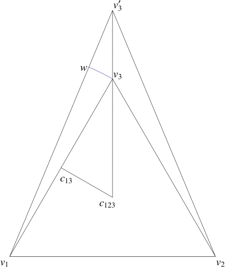
Figure 1: Variation of a triangle.

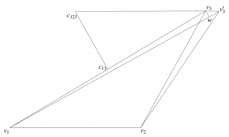
Figure 2: Variation of a triangle where $c_{123}$ is outside the triangle.

In this section we will compute the derivative of an angle under a certain variation of lengths. Consider the Euclidean triangle determined by lengths $\left(\ell_{12},\ell_{13},\ell_{23}\right)$ with vertices $\left\{v_{1},v_{2},v_{3}\right\}$ and also the triangle determined by lengths $\left(\ell_{12},\ell_{13}+\delta\ell_{13},\ell_{23}+\delta\ell_{23}\right)$, say with vertices $\left\{v_{1},v_{2},v_{3}^{\prime}\right\}$, under the important assumptions:

$$\delta\ell_{12} =0,$$ (17)

$$\delta\ell_{13} =d_{31}\delta f_{3},$$ (18)

$$\delta\ell_{23} =d_{32}\delta f_{3},$$ (19)

where $d$ is a metric on $\left\{1,2,3\right\}$ inducing lengths $\ell.$

Draw the arc representing $\ell_{14}~{}\delta\gamma_{1,24},$ which goes through vertex $v_{3}$ and intersects the segment $v_{1}v_{3}^{\prime}.$ Call this edge $E.$ It has endpoints $v_{3}$ and $w.$ See Figures 1 and 2 for cases when the center $c_{123}$ is inside $v_{1}v_{2}v_{3}$ and when it is outside $v_{1}v_{2}v_{3}$.

Proposition 28

The points $c_{123},$ $v_{3},$ and $v_{3}^{\prime}$ lie on a line. I.e., $\delta v_{3}$ is parallel to $v_{3}-c_{123}.$

Proof. Notice that

$$\delta\left(\ell_{13}^{2}\right)=\delta\left[\left(v_{3}-v_{1}\right)\cdot\left(v_{3}-v_{1}\right)\right]=2\left(v_{3}-v_{1}\right)\cdot\delta v_{3}$$

but also

$$\delta\left(\ell_{13}^{2}\right)=2\ell_{13}d_{31}\delta f_{3},$$

so

$$\delta v_{3}\cdot\frac{v_{3}-v_{1}}{\ell_{13}}=d_{31}\delta f_{3}.$$

Similarly,

$$\delta v_{3}\cdot\frac{v_{3}-v_{2}}{\ell_{23}}=d_{32}\delta f_{3}.$$

Similarly, the vector $v_{3}-c_{123}$ satisfies

$$\left(v_{3}-c_{123}\right)\cdot\frac{v_{3}}{\ell_{13}} =d_{31},$$

$$\left(v_{3}-c_{123}\right)\cdot\frac{v_{3}-v_{2}}{\ell_{23}} =d_{32}$$

and so we see that $\delta v_{3}=\left(v_{3}-c_{123}\right)\delta f_{3}.$   

This is essentially the same proof given by Thurston [44] and Marden-Rodin [29].

Consider the triangle $v_{3}wv_{3^{\prime}}.$ This is a right triangle with right angle at $w$ since $v_{1}w$ is a radius of the circle containing $E.$ Since the angle of $E$ with $v_{1}v_{3}$ is also a right angle, together with Proposition 28, it follows that $v_{3}wv_{3^{\prime}}$ is similar to the right triangle $c_{123}c_{13}v_{3}$. Using the similar triangles, we get that

$$\frac{\ell_{13}\left(\delta\gamma_{1,23}\right)}{\delta\ell_{13}}=\frac{h_{13,2}}{d_{31}}.$$ (20)

So

$$\frac{\partial\gamma_{1,23}}{\partial f_{3}}=\frac{h_{13,2}}{\ell_{13}}.$$

This leads to the following theorem.

Theorem 29

For variations of the lengths of a Euclidean triangle of the type 17-19 (where $\delta f_{3}$ is arbitrary), we have

$$\frac{\partial\gamma_{1,23}}{\partial f_{3}} =\frac{h_{13,2}}{\ell_{13}}$$

$$\frac{\partial\gamma_{2,13}}{\partial f_{3}} =\frac{h_{23,1}}{\ell_{23}}$$

$$\frac{\partial\gamma_{3,12}}{\partial f_{3}} =-\frac{h_{13,2}}{\ell_{13}}-\frac{h_{23,1}}{\ell_{23}}.$$

Proof. We have already proven the first two equalities. The last follows from the fact that in a Euclidean triangle, $\gamma_{1,23}+\gamma_{2,13}+\gamma_{3,12}=\pi.$   

Remark 30

Special cases of this theorem appear in [23][17][18][19] and less refined versions (where only signs and not explicit values are computed for the derivatives) appear in many other places, including [44][39][29][43].

3.2 Three dimensions

Now consider a tetrahedron $\left\{1,2,3,4\right\}$. Similarly, we will need variations of the form

$$\delta\ell_{12} =0,$$ (21)

$$\delta\ell_{13} =0,$$ (22)

$$\delta\ell_{23} =0,$$ (23)

$$\delta\ell_{14} =d_{41}\delta f_{4},$$ (24)

$$\delta\ell_{24} =d_{42}\delta f_{4},$$ (25)

$$\delta\ell_{34} =d_{43}\delta f_{4},$$ (26)

where $d$ is a metric on $\left\{1,2,3,4\right\}$. For convenience, we embed the vertices of the tetrahedron as $\left\{v_{1},v_{2},v_{3},v_{4}\right\}$ so that it has the correct edge lengths and such that $v_{1}$ is at the origin, $v_{2}$ is along the positive $x$-axis, $v_{3}$ is in the $xy$-plane, and $v_{4}$ is above the $xy$-plane. We will need some additional points. We let $v_{4}^{\prime}$ be the new vertex $4$ gotten by taking lengths $\ell_{ij}+\delta\ell_{ij}$ (remembering that, for instance, $\delta\ell_{12}=0$) and embedding this tetrahedron as $v_{1}v_{2}v_{3}v_{4}^{\prime},$ with $v_{4}^{\prime}$ above the $xy$-plane. We also need $v_{4,12}^{\prime}$ which is the point on the plane $v_{1}v_{2}v_{4}^{\prime}$ which makes $v_{1}v_{2}v_{4,12}^{\prime}$ a triangle congruent to $v_{1}v_{2}v_{4}.$ Also, we have the point $v_{4,1}^{\prime},$ which is the point on the line $v_{1}v_{4}^{\prime}$ which is a distance $\ell_{14}$ from $v_{1}.$ See Figure 3.

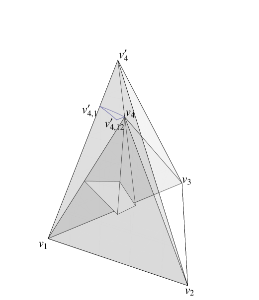
Figure 3: Variation of a tetrahedron.

We first observe that the right tetrahedron $v_{4}v_{4,12}^{\prime}v_{4,1}^{\prime}v_{4}^{\prime}$ is similar to the tetrahedron $c_{1234}c_{124}c_{14}v_{4}.$ This is because $c_{1234},$ $v_{4},$ and $v_{4}^{\prime}$ are colinear (the proof is exactly analogous to the proof of Proposition 28, and is thus omitted). This implies that

$$\frac{\left(\delta\ell_{14}\right)^{2}}{d_{41}^{2}}=\frac{\frac{1}{2}\left(\ell_{14}\delta\gamma_{1,24}\right)\left(\ell_{14}\sin\gamma_{1,24}\left(\delta\beta_{12,34}\right)\right)}{\frac{1}{2}h_{14,2}h_{124,3}}.$$

We conclude that

$$\frac{h_{124,3}h_{14,2}}{d_{41}^{2}\sin\gamma_{1,24}\ell_{14}} =\frac{\delta\gamma_{1,24}}{\delta\ell_{14}}\ell_{14}\left(\frac{\delta\beta_{12,34}}{\delta\ell_{14}}\right)$$

$$=\frac{h_{14,2}}{d_{41}}\left(\frac{\delta\beta_{12,34}}{\delta\ell_{14}}\right)$$

using Theorem 29. We thus get

$$\frac{h_{124,3}}{d_{41}\sin\gamma_{1,24}\ell_{14}}=\frac{\delta\beta_{12,34}}{\delta\ell_{14}}.$$ (27)

Furthermore, if $\alpha_{1}$ is the solid angle at vertex $v_{1},$ then we get that $\ell_{14}^{2}\delta\alpha_{1}$ is approximately the sum of the areas of two triangles on the sphere centered at $v_{1}$ of radius $\ell_{14}.$ One triangle has vertices $v_{4,1}^{\prime},v_{4},$ and a point on the $x$-axis which we will call $b.$ See Figure 4.

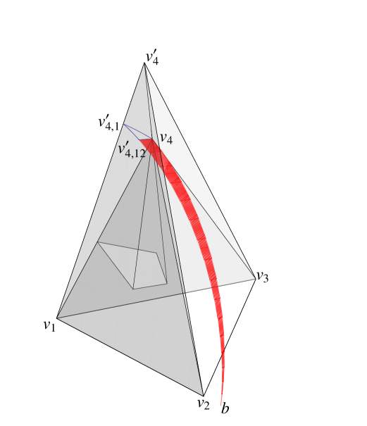
Figure 4: Angle variation setup for a tetrahedron.

This triangle can be divided into two spherical triangles, $v_{4,1}^{\prime}v_{4,12}^{\prime}v_{4}$ and $v_{4,12}^{\prime}v_{4}b.$ Each of these triangles has a right angle at $v_{4,12}^{\prime}.$ Note that the first triangle has area which vanishes to higher order, so up to first order, the area is the area of the second triangle. This triangle has a right angle at $v_{4,12}^{\prime},$ has angle $\delta\beta_{12,34}$ at $b,$ and some other angle at $v_{4}$, say $\frac{\pi}{2}-\gamma,$ where $\gamma$ is small. It is easy to see that the side $v_{4,12}^{\prime}b$ in the spherical triangle has length $\ell_{14}\delta\gamma_{1,24}$ and the side $v_{4,12}^{\prime}v_{4}$ has length $\ell_{14}\sin\gamma_{1,24}\delta\beta_{12,34}$ to first order (the error is like $\left(\delta\beta_{12,34}\right)^{3}$). We may compute $\gamma$ since we know by spherical trigonometry that

$$\cos\left(\frac{\pi}{2}-\gamma\right)=\frac{\tan\left(\delta\beta_{12,34}\sin\gamma_{1,24}\right)}{\tan\gamma_{1,24}}.$$

We look at this asymptotically where $\delta\beta_{12,34}$ is small, and see that

$$\gamma=\frac{\delta\beta_{12,34}\sin\gamma_{1,24}}{\tan\gamma_{1,24}}=\delta\beta_{12,34}\cos\gamma_{1,24}$$

and thus the area of the triangle is

$$\ell_{14}^{2}\left(\delta\beta_{12,34}+\frac{\pi}{2}+\frac{\pi}{2}-\delta\beta_{12,34}\cos\gamma_{1,24}-\pi\right)$$

$$=\ell_{14}^{2}\delta\beta_{12,34}\left(1-\cos\gamma_{1,24}\right).$$

Hence we have that

$$\delta\alpha_{1}=\delta\beta_{12,34}+\delta\beta_{13,24}+\delta\beta_{14,23}$$

implies that

$$\delta\beta_{12,34}\left(1-\cos\gamma_{1,24}\right)+\delta\beta_{13,24}\left(1-\cos\gamma_{1,34}\right)=\delta\beta_{12,34}+\delta\beta_{13,24}+\delta\beta_{14,23}$$

or

$$\delta\beta_{14,23} =-\cos\gamma_{1,24}\delta\beta_{12,34}-\cos\gamma_{1,34}\delta\beta_{13,24}$$

$$=-\cos\gamma_{1,24}\frac{h_{124,3}}{d_{41}\sin\gamma_{1,24}\ell_{14}}\delta\ell_{14}-\cos\gamma_{1,34}\frac{h_{134,2}}{d_{41}\sin\gamma_{1,34}\ell_{14}}\delta\ell_{14}$$

$$=-\frac{1}{d_{41}\ell_{14}}\left(\cot\gamma_{1,24}h_{124,3}+\cot\gamma_{1,34}h_{134,2}\right)\delta\ell_{14}$$

$$=\frac{1}{d_{14}d_{41}\ell_{14}}\left(h_{14,2}h_{124,3}+h_{14,3}h_{134,2}-\frac{d_{12}h_{124,3}}{\sin\gamma_{1,24}}-\frac{d_{13}h_{134,2}}{\sin\gamma_{1,34}}\right)\delta\ell_{14}.$$

Recalling that

$$\frac{h_{124,3}}{d_{41}\sin\gamma_{1,24}\ell_{14}}=\frac{\delta\beta_{12,34}}{\delta\ell_{14}}$$

we get

$$d_{41}\left(d_{14}\delta\beta_{14,23}+d_{12}\delta\beta_{12,34}+d_{13}\delta\beta_{13,24}\right)$$

$$=\frac{1}{\ell_{14}}\left(h_{14,2}h_{124,3}+h_{14,3}h_{134,2}\right)\delta\ell_{14}$$

$$=2\frac{A_{14,23}}{\ell_{14}}\delta\ell_{14}=2\frac{A_{14,23}}{\ell_{14}}d_{41}\delta f_{4}.$$ (28)

That is,

$$d_{14}\delta\beta_{14,23}+d_{12}\delta\beta_{12,34}+d_{13}\delta\beta_{13,24}=2\frac{A_{14,23}}{\ell_{14}}\delta f_{4}.$$

Furthermore, the Schläfli formula implies that in the tetrahedron,

$$\ell_{12}\delta\beta_{12}+\ell_{13}\delta\beta_{13}+\ell_{14}\delta\beta_{14}+\ell_{23}\delta\beta_{23}+\ell_{24}\delta\beta_{24}+\ell_{34}\delta\beta_{34}=0,$$

and so

$$0 =\left(d_{14}\delta\beta_{14}+d_{12}\delta\beta_{12}+d_{13}\delta\beta_{13}\right)+\left(d_{21}\delta\beta_{12}+d_{23}\delta\beta_{23}+d_{24}\delta\beta_{24}\right)$$

$$\;\;\;\;+\left(d_{31}\delta\beta_{13}+d_{32}\delta\beta_{23}+d_{34}\delta\beta_{34}\right)+\left(d_{41}\delta\beta_{14}+d_{42}\delta\beta_{24}+d_{43}\delta\beta_{34}\right).$$

The first three terms are all of the form (28) and the last is different (because the lengths of edges around vertex $4$ are changing). Thus,

$$\left(d_{41}\delta\beta_{14}+d_{42}\delta\beta_{24}+d_{43}\delta\beta_{34}\right) =-2\frac{A_{14,23}}{d_{41}\ell_{14}}\delta\ell_{14}-2\frac{A_{24,13}}{d_{42}\ell_{24}}\delta\ell_{24}-2\frac{A_{34,12}}{d_{43}\ell_{34}}\delta\ell_{34}$$

$$=\left[-2\frac{A_{14,23}}{\ell_{14}}-2\frac{A_{24,13}}{\ell_{24}}-2\frac{A_{34,12}}{\ell_{34}}\right]\delta f_{4}.$$

We have just proven the following theorem.

Theorem 31

Under variations of the form (21)-(26), we have

$$d_{14}\delta\beta_{14}+d_{12}\delta\beta_{12}+d_{13}\delta\beta_{13} =2\frac{A_{14,23}}{\ell_{14}}\delta f_{4},$$

$$d_{24}\delta\beta_{24}+d_{23}\delta\beta_{23}+d_{21}\delta\beta_{12} =2\frac{A_{24,13}}{\ell_{24}}\delta f_{4},$$

$$d_{34}\delta\beta_{34}+d_{32}\delta\beta_{23}+d_{31}\delta\beta_{13} =2\frac{A_{34,12}}{\ell_{34}}\delta f_{4},$$

$$d_{41}\delta\beta_{14}+d_{42}\delta\beta_{24}+d_{43}\delta\beta_{34} =\left[-2\frac{A_{14,23}}{\ell_{14}}-2\frac{A_{24,13}}{\ell_{24}}-2\frac{A_{34,12}}{\ell_{34}}\right]\delta f_{4}.$$

We actually derived a finer result, with explicit computation of the variations of individual dihedral angles. However, the result in this form is more compactly stated and all we will use in the remainder of this paper. Also, this result was derived in [17] for the specific case of sphere-packing configurations of a tetrahedron. Less precise results along these lines were examined in the sphere-packing case in [12][37] as well. We will go into more detail later.

4 Curvature variations

4.1 Two dimensions

Discrete curvature in two dimensions has been well studied, with curvature as in Definition 11. Theorem 29 has the following implication.

Theorem 32

Let $f\left(t\right)$ be a conformal variation of $\left(M^{2},T,d\right)$ Then for $t=0,$

$$\frac{dK_{i}}{dt}=-\sum_{j}\frac{\ell_{ij}^{\ast}}{\ell_{ij}}\left(\frac{df_{j}}{dt}-\frac{df_{i}}{dt}\right).$$ (29)

Proof. We compute

$$\frac{dK_{i}}{dt} =\frac{d}{dt}\left(2\pi-\sum_{j,k}\gamma_{i,jk}\right)$$

$$=-\sum_{j,k}\left(\frac{\partial\gamma_{i,jk}}{\partial f_{i}}\frac{df_{i}}{dt}+\frac{\partial\gamma_{i,jk}}{\partial f_{j}}\frac{df_{j}}{dt}+\frac{\partial\gamma_{i,jk}}{\partial f_{k}}\frac{df_{k}}{dt}\right)$$

$$=-\sum_{j,k}\left[\frac{h_{ij,k}}{\ell_{ij}}\left(\frac{df_{j}}{dt}-\frac{df_{i}}{dt}\right)+\frac{h_{ik,j}}{\ell_{ik}}\left(\frac{df_{k}}{dt}-\frac{df_{i}}{dt}\right)\right],$$

which implies the result.   

Remark 33

We will express many of the variation results as in Theorem 32 instead of in terms of $\frac{\partial K_{i}}{\partial f_{j}}$ in order to emphasize the presence of the Laplacian. Notice that the formula (29) has the form

$$\frac{dK_{i}}{dt}=-\left(\triangle\frac{df}{dt}\right)_{i}$$

for an appropriate definition of the Laplacian $\triangle$. We will comment more on this in Section 6.

The formulas from Theorem 29 also imply that the curvatures are variational giving the proof of Theorem 23.

Proof of Theorem 23. $F$ will be defined as

$$F\left(f\right)=\int_{f_{0}}^{f}\omega$$

for the $1$-form

$$\omega=\sum K_{i}df_{i}.$$

To ensure that the integral is independent of path, we need that $\omega$ is closed. Since we are in a simply connected domain, we need only check that

$$\frac{\partial K_{i}}{\partial f_{j}}=\frac{\partial K_{j}}{\partial f_{i}}$$

for $i\neq j.$ We can compute these derivative explicitly, and they are

$$\frac{\partial K_{i}}{\partial f_{j}}=-\frac{\ell_{ij}^{\ast}}{\ell_{ij}}=\frac{\partial K_{j}}{\partial f_{i}}$$

if $i$ and $j$ share an edge and zero otherwise.   

This formulation of the prescribed curvature problem in a variational framework has been studied by many people. See, for instance, [13] [36] [11] [9] [41] [21], many of which derive the functional in precisely the same way. Certain conformal variations in the discrete setting have been proposed by Roček and Williams in the context of Regge calculus [38], Thurston in the setting of circle patterns [44] (see also other work on circle packing, e.g., [43]), and Luo [28] (see also [42]). Our current setting takes each of these definitions and proofs as special cases (see Section 5). In many of these papers it is shown that the largest “reasonable” domain for the $f$’s is simply connected. The advantage of Theorem 23 is that it works for a more general class of conformal variations. In addition, we have a geometric description of the derivatives $\frac{\partial K_{i}}{\partial f_{j}}$ which is absent from most of these previous works.

4.2 Three dimensions and the Einstein-Hilbert-Regge functional

We could follow a similar method to that in Theorem 23 to prove that there are three-dimensional curvatures which are variational. However, we will present this fact in a different way by using the Einstein-Hilbert-Regge functional from Definition 13.

Recall Definition 15 for scalar curvatures in dimension three. The definition is first motivated by seeing how the Schläfli formula decomposes as sums around vertices. The Schläfli formula on a tetrahedron is

$$\sum_{i,j}\ell_{ij}\delta\beta_{ij}=0,$$

where the sum is over all edges $\left\{i,j\right\}$ in the tetrahedron. It can be written as

$$0 =\left(d_{12}+d_{21}\right)\delta\beta_{12}+\left(d_{13}+d_{31}\right)\delta\beta_{13}+\left(d_{14}+d_{41}\right)\delta\beta_{14}$$

$$\;\;\;+\left(d_{23}+d_{32}\right)\delta\beta_{23}+\left(d_{24}+d_{42}\right)\delta\beta_{24}+\left(d_{34}+d_{43}\right)\delta\beta_{34}$$

$$=\left(d_{12}\delta\beta_{12}+d_{13}\delta\beta_{13}+d_{14}\delta\beta_{14}\right)+\left(d_{21}\delta\beta_{12}+d_{23}\delta\beta_{23}+d_{24}\delta\beta_{24}\right)$$

$$\;\;\;+\left(d_{31}\delta\beta_{13}+d_{32}\delta\beta_{23}+d_{34}\delta\beta_{34}\right)+\left(d_{41}\delta\beta_{14}+d_{42}\delta\beta_{24}+d_{43}\delta\beta_{34}\right),$$

giving the vertex breakdown motivating the curvature formula. The Schläfli formula allows an easy computation of first derivatives of the Einstein-Hilbert-Regge functional on a triangulation of a closed manifold, giving

$$\frac{\partial}{\partial f_{i}}\mathcal{EHR}\left(T,\ell\left(f\right)\right) =\frac{\partial}{\partial f_{i}}\left[\sum_{i,j}\left(2\pi-\sum_{k,\ell}\beta_{ij,k\ell}\right)\ell_{ij}\right]$$

$$=\sum_{j}\left(2\pi-\sum_{k,\ell}\beta_{ij,k\ell}\right)d_{ij}$$ (30)

$$=K_{i}.$$

To compute the second variation, we need the variation of $K_{i}.$ Using Theorem 31 we can express the derivatives of curvature.

Theorem 34

Let $f\left(t\right)$ be a conformal variation of $\left(M^{3},T,d\right).$ Then,

$$\frac{dK_{i}}{dt} =-2\sum_{j\neq i}\frac{\ell_{ij}^{\ast}}{\ell_{ij}}\left(\frac{df_{j}}{dt}-\frac{df_{i}}{dt}\right)+\sum_{j\neq i}\left(2\pi-\sum_{k,\ell}\beta_{ij,k\ell}\right)\frac{d}{dt}d_{ij}$$ (31)

$$=-\sum_{j\neq i}\left(2\frac{\ell_{ij}^{\ast}}{\ell_{ij}}-\frac{q_{ij}}{\ell_{ij}}K_{ij}\right)\left(\frac{df_{j}}{dt}-\frac{df_{i}}{dt}\right)+K_{i}\frac{df_{i}}{dt},$$

where

$$q_{ij}=\frac{\partial d_{ij}}{\partial f_{j}}=\frac{\partial d_{ji}}{\partial f_{i}}.$$

We note that the first term in (31) is the Laplacian operator studied by the author in [19].

Proof. We compute

$$\frac{d}{dt}K_{i} =2\pi\sum_{j}\frac{d}{dt}d_{ij}-2\sum_{j\neq i}\frac{\ell_{ij}^{\ast}}{\ell_{ij}}\left(\frac{df_{j}}{dt}-\frac{df_{i}}{dt}\right)$$

$$\;\;\;-\sum_{j,k,\ell}\left(\beta_{ij,k\ell}\frac{d}{dt}d_{ij}+\beta_{ik,j\ell}\frac{d}{dt}d_{ik}+\beta_{i\ell,jk}\frac{d}{dt}d_{i\ell}\right)$$

$$=-2\sum_{j\neq i}\frac{\ell_{ij}^{\ast}}{\ell_{ij}}\left(\frac{df_{j}}{dt}-\frac{df_{i}}{dt}\right)+\sum_{j\neq i}\left(2\pi-\sum_{k,\ell}\beta_{ij,k\ell}\right)\frac{d}{dt}d_{ij}.$$

Furthermore, if there is a conformal structure, then

$$\frac{\partial d_{ij}}{\partial f_{j}}=\frac{\partial}{\partial f_{j}}\frac{\partial\ell_{ij}}{\partial f_{i}}=\frac{\partial}{\partial f_{i}}\frac{\partial\ell_{ij}}{\partial f_{j}}=\frac{\partial d_{ji}}{\partial f_{i}}.$$

Thus

$$q_{ij}=\frac{\partial d_{ij}}{\partial f_{j}}=\frac{\partial d_{ji}}{\partial f_{i}}=\frac{\partial^{2}\ell_{ij}}{\partial f_{i}\partial f_{j}}$$

is symmetric, i.e., $q_{ij}=q_{ji}.$ This also implies that

$$\frac{\partial d_{ij}}{\partial f_{i}} =\frac{\partial\ell_{ij}}{\partial f_{i}}-\frac{\partial d_{ji}}{\partial f_{i}}$$

$$=d_{ij}-q_{ij}.$$

Thus

$$\frac{d}{dt}d_{ij}=\left(d_{ij}-q_{ij}\right)\frac{df_{i}}{dt}+q_{ij}\frac{df_{j}}{dt}.$$

The result follows.   

We can compute the variations of the Einstein-Hilbert-Regge functional.

Proof of Theorem 24. Using (30), we see immediately that

$$\frac{d}{dt}\mathcal{EHR}\left(M,T,\ell\left(f\left(t\right)\right)\right)=\sum_{i\in V}K_{i}\frac{df_{i}}{dt}.$$

Using Theorem 34, we compute that

$$\frac{d^{2}}{dt^{2}}\mathcal{EHR}\left(M,T,\ell\left(f\left(t\right)\right)\right) =\sum_{i}\frac{dK_{i}}{dt}\frac{df_{i}}{dt}+K_{i}\frac{d^{2}f_{i}}{dt^{2}}$$

$$=-\sum_{i}\sum_{j\neq i}\left(2\frac{\ell_{ij}^{\ast}}{\ell_{ij}}-\frac{q_{ij}}{\ell_{ij}}K_{ij}\right)\left(\frac{df_{j}}{dt}-\frac{df_{i}}{dt}\right)\frac{df_{i}}{dt}$$

$$\;\;\;\;\;\;\;+\sum_{i}K_{i}\left[\left(\frac{df_{i}}{dt}\right)^{2}+\frac{d^{2}f_{i}}{dt^{2}}\right]$$

$$=\sum_{i}\sum_{j\neq i}\left(\frac{\ell_{ij}^{\ast}}{\ell_{ij}}-\frac{q_{ij}}{2\ell_{ij}}K_{ij}\right)\left(\frac{df_{j}}{dt}-\frac{df_{i}}{dt}\right)^{2}$$

$$\;\;\;\;\;\;\;+\sum_{i}K_{i}\left[\left(\frac{df_{i}}{dt}\right)^{2}+\frac{d^{2}f_{i}}{dt^{2}}\right].$$

The rest of the theorem follows immediately from (30) and Regge’s variation formula (8).   

In order to get better control of $q_{ij}$, we will look at special conformal structures in Section 5.

Finally we can complete the proof of Corollary 25.

Proof of Corollary 25. We see from Figure 3 that we must have that if we fix $f_{1},f_{2},f_{3}$ and let $f_{4}$ vary, then

$$\delta V_{1234} =\frac{1}{3}A_{124}\ell_{14}\sin\gamma_{1,24}\delta\beta_{12,34}+\frac{1}{3}A_{134}\ell_{14}\sin\gamma_{1,34}\delta\beta_{13,24}$$

$$\;\;\;\;\;\;+\frac{1}{3}A_{234}\ell_{34}\sin\gamma_{3,24}\delta\beta_{23,14}$$

$$=\frac{1}{3}\left(A_{124}h_{124,3}+A_{134}h_{134,2}+A_{234}h_{234,1}\right)$$

by (27), which implies that

$$\frac{\partial}{\partial f_{i}}\mathcal{V}\left(T,\ell\left(f\right)\right)=V_{i}$$

where

$$V_{i}=\frac{1}{3}\sum_{j,k,\ell}h_{ijk,\ell}A_{ijk}$$

and the sum is over all tetrahedra containing $i$ and all faces in those tetrahedra containing $i.$   

5 Examples of conformal structures

In this section we place previously studied geometric structures into the framework of conformal structures.

5.1 Circle and sphere packing

The case of circle packing and sphere packing is when edge lengths arise from spheres centered at the vertices which are externally tangent to each other. In this case, there are positive weights $r_{i}$ corresponding to the radii and $\ell_{ij}=r_{i}+r_{j}$. In two dimensions, circle packings have been considered in a number of contexts; see Stephenson’s monograph [43] for an overview. In three dimensions, this case was considered by Cooper-Rivin [12]. They noticed, in particular, that for a sphere packing, one can rewrite the Schläfli formula in the following way:

$$0 =\left(r_{1}+r_{2}\right)\delta\beta_{12}+\left(r_{1}+r_{3}\right)\delta\beta_{13}+\left(r_{1}+r_{4}\right)\delta\beta_{14}$$

$$\;\;\;+\left(r_{2}+r_{3}\right)\delta\beta_{23}+\left(r_{2}+r_{4}\right)\delta\beta_{24}+\left(r_{3}+r_{4}\right)\delta\beta_{34}$$

$$=r_{1}\left(\delta\beta_{12}+\delta\beta_{13}+\delta\beta_{14}\right)+r_{2}\left(\delta\beta_{12}+\delta\beta_{23}+\delta\beta_{24}\right)$$

$$\;\;\;+r_{3}\left(\delta\beta_{13}+\delta\beta_{23}+\delta\beta_{34}\right)+r_{4}\left(\delta\beta_{14}+\delta\beta_{24}+\delta\beta_{34}\right)$$

$$=r_{1}\delta\alpha_{1}+r_{2}\delta\alpha_{2}+r_{3}\delta\alpha_{3}+r_{4}\delta\alpha_{4},$$

where $\alpha_{i}$ is the solid angle at vertex $i,$ and thus $\delta\alpha_{1}=\delta\left(\beta_{12}+\beta_{13}+\beta_{14}-\pi\right)=$ $\delta\beta_{12}+\delta\beta_{13}+\delta\beta_{14}.$ They used this to motivate the definition of scalar curvature as $4\pi-\sum\alpha_{i}$ where the sum is over all tetrahedra containing $i$ as a vertex. From our setting, we would define the scalar curvature measure instead as

$$K_{i}=\left(4\pi-\sum_{j,k,\ell}\alpha_{i,jk\ell}\right)r_{i}=\sum_{j}\left(2\pi-\sum_{k,\ell}\beta_{ij,k\ell}\right)r_{i},$$

where in the right side, the first sum is over all edges incident on $i$ and the second sum is the sum over all tetrahedra containing $\left\{i,j\right\}$ as an edge. The second equality can be easily derived using the Euler characteristic and area formula of the sphere centered at vertex $i.$

To match this to our setting, we see that we must take $f_{i}=\log r_{i}$ and $d_{ij}=r_{i},$ since

$$\ell_{ij} =r_{i}+r_{j}$$

$$\frac{\partial\ell_{ij}}{\partial r_{i}}r_{i} =r_{i}.$$

Thus we have the following conformal structure.

Definition 35

The circle/sphere packing conformal structure, $\mathcal{C}^{P}\left(M,T\right),$ is the map defining

$$d_{ij}=e^{f_{i}}$$

for every oriented edge in $E_{+}\left(T\right)$ restricted to an appropriate domain of $f\in V^{\ast}\left(T\right).$

In two dimensions, the triangle inequality is automatically satisfied, and so the domain is all of $V^{\ast}\left(T\right).$ In three dimensions, there is an additional condition that the square volumes of three-dimensional simplices (as defined by the Cayley-Menger determinant formula) are positive. This is discussed in some detail in [17] [18].

We see that the formulas in Section 3.2 correspond to

$$\frac{\partial\alpha_{1}}{\partial r_{4}}r_{1}r_{4}=2\frac{A_{14,23}}{\ell_{14}}.$$

This is the same formula derived by the author in [17].

5.2 Fixed intersection angles/inversive distance

There is a more general case of circles or spheres with fixed intersection angles, originally considered by Thurston [44]. Here we parametrize lengths by two parameters, radii $r_{i}$ and inversive distances $\eta_{ij}$. The inversive distance (see, for instance, [21]) is like the cosine of the supplement of the intersection angle, defined so that

$$\ell_{ij}^{2}=r_{i}^{2}+r_{j}^{2}+2r_{i}r_{j}\eta_{ij}.$$

We will use this formula to parametrize the lengths by the radii $r_{i}$ with inversive distances fixed. It essentially corresponds to having circles at the vertices of radius $r_{i}$ and intersecting at angle $\arccos\left(-\eta_{ij}\right).$ If $\eta_{ij}$ is not between $-1$ and $1,$ then the circles may not intersect, but this is not a problem for the theory. There is always a circle orthogonal to these circles, and we take the center of the triangle to be the center of this orthocircle. (Note, it is possible that this circle does not have real radius, but the center is still well defined using the algebra of circles given in [32].) We then find that

$$d_{ij}=\frac{r_{i}\left(r_{i}+r_{j}\eta_{ij}\right)}{\ell_{ij}}.$$ (32)

For a path in the $r$ variables, we compute

$$\ell_{ij}\frac{d}{dt}\ell_{ij} =\left(r_{i}+r_{j}\eta_{ij}\right)\frac{dr_{i}}{dt}+\left(r_{j}+r_{i}\eta_{ij}\right)\frac{dr_{j}}{dt}$$

$$\frac{d}{dt}\ell_{ij} =d_{ij}\frac{1}{r_{i}}\frac{dr_{i}}{dt}+d_{ji}\frac{1}{r_{j}}\frac{dr_{j}}{dt}.$$

Thus we see that $f_{i}=\log r_{i},$ giving the fixed inversive distance conformal class.

Definition 36

For a given $\eta\in E\left(T\right)^{\ast},$ the fixed inversive distance conformal structure, $\mathcal{C}^{FI}\left(M,T,\eta\right),$ is the conformal structure described by the map

$$d_{ij}=\frac{e^{f_{i}}\left(e^{f_{i}}+e^{f_{j}}\eta_{ij}\right)}{\ell_{ij}\left(f\right)},$$

where

$$\ell_{ij}\left(f\right)=\sqrt{e^{2f_{i}}+e^{2f_{j}}+2e^{f_{i}}e^{f_{j}}\eta_{ij}}$$

is the length, when restricted to a proper domain in $V\left(T\right)^{\ast}$

Note that there are some restrictions on the domain which may be quite complicated, including the triangle inequality. However, it has been found that in two dimensions, if $\eta_{ij}\geq 0$ for all $\eta\in E\left(T\right)^{\ast},$ then the domain is simply connected. This was initially shown for $0\leq\eta_{ij}\leq 1$ by Thurston ([44] [29]) and the additional cases were proven recently by Guo [21].

We see that

$$q_{ij} =\frac{\partial d_{ij}}{\partial f_{j}}=r_{j}\frac{\partial d_{ij}}{\partial r_{j}}$$

$$=\frac{r_{i}^{2}r_{j}^{2}\left(\eta_{ij}^{2}-1\right)}{\ell_{ij}^{3}}.$$

We finally get

$$\frac{dK_{i}}{dt}=-\sum_{j\neq i}\left(2\frac{\ell_{ij}^{\ast}}{\ell_{ij}}-\frac{r_{i}^{2}r_{j}^{2}\left(1-\eta_{ij}^{2}\right)}{\ell_{ij}^{4}}K_{ij}\right)\left(\frac{df_{j}}{dt}-\frac{df_{i}}{dt}\right)+K_{i}\frac{df_{i}}{dt},$$

and the second variation of the Einstein-Hilbert-Regge functional is

$$\frac{d^{2}}{dt^{2}}\mathcal{EHR}\left(T,\ell\left(f\left(t\right)\right)\right) =\sum_{i}\sum_{j\neq i}\left(\frac{\ell_{ij}^{\ast}}{\ell_{ij}}-\frac{r_{i}^{2}r_{j}^{2}\left(1-\eta_{ij}^{2}\right)}{2\ell_{ij}^{4}}K_{ij}\right)\left(\frac{df_{j}}{dt}-\frac{df_{i}}{dt}\right)^{2}$$

$$\;\;\;+\sum_{i}K_{i}\left[\left(\frac{df_{i}}{dt}\right)^{2}+\frac{d^{2}f_{i}}{dt^{2}}\right].$$

Note that in the case that $\eta_{ij}=1,$ corresponding to sphere packing, the second term is zero. In general, for spheres with intersection we have $\eta_{ij}\leq 1$ and for spheres which do not intersect we have $\eta_{ij}>1$ and so in each case the term with edge curvatures has a particular sign.

5.3 Perpendicular bisectors

Here we give the conformal structure proposed by Roček-Williams [38], Luo [28], and Pinkall-Schroeder-Springborn [42]. This structure has also been found in the numerical analysis literature on approximations of the Laplacian in the context of the box method (see, e.g., [25] and [34]). Take

$$\ell_{ij}=e^{u_{i}+u_{j}}L_{ij}$$

where $L_{ij}$ are fixed lengths. We see that, given a path in the space of $u$ variables,

$$\frac{d}{dt}\ell_{ij}=\ell_{ij}\left(\frac{du_{i}}{dt}+\frac{du_{j}}{dt}\right).$$

If we take

$$d_{ij} =\frac{\ell_{ij}}{2}$$

$$f_{i} =2u_{i}$$

then

$$\frac{d}{dt}\ell_{ij}=d_{ij}\frac{df_{i}}{dt}+d_{ji}\frac{df_{j}}{dt}.$$

We notice that the duals to the edges intersect the edges at their midpoints, which is why we call this the perpendicular bisector conformal structure following [25]. It can be proven inductively that the center of any simplex is the center of the sphere circumscribing that simplex.

Definition 37

Let $L\in E\left(T\right)$ be such that $\left(M,T,L\right)$ is a piecewise flat manifold. The perpendicular bisector conformal structure, $\mathcal{C}^{PB}\left(M,T,L\right),$ is the conformal structure determined by

$$d_{ij}=\frac{1}{2}e^{\frac{1}{2}\left(f_{i}+f_{j}\right)}L_{ij},$$

when restricted to an appropriate domain.

Since $\left(M,T,d\left(\vec{0}\right)\right)$ is a piecewise flat, metrized manifold, this conformal structure exists for $f_{i}$ close to $0.$ However, the largest possible domain must satisfy a number of inequalities.

We see that

$$q_{ij}=\frac{\partial d_{ij}}{\partial f_{j}}=\frac{1}{4}\ell_{ij}.$$

Thus, in three dimensions the variation of curvature is

$$\frac{dK_{i}}{dt}=-\sum_{j\neq i}\left(2\frac{\ell_{ij}^{\ast}}{\ell_{ij}}-\frac{1}{4}K_{ij}\right)\left(\frac{df_{j}}{dt}-\frac{df_{i}}{dt}\right)+K_{i}\frac{df_{i}}{dt}.$$

We get that

$$\frac{d^{2}}{dt^{2}}\mathcal{EHR}\left(T,\ell\left(f\left(t\right)\right)\right) =\sum_{i}\sum_{j\neq i}\left(\frac{\ell_{ij}^{\ast}}{\ell_{ij}}-\frac{1}{8}K_{ij}\right)\left(\frac{df_{j}}{dt}-\frac{df_{i}}{dt}\right)^{2}$$

$$\;\;\;\;\;\;\;+\sum_{i}K_{i}\left[\left(\frac{df_{i}}{dt}\right)^{2}+\frac{d^{2}f_{i}}{dt^{2}}\right].$$

6 The discrete Laplacian and the second variation

6.1 Laplacians

The relationship between the second variation of the functionals presented here and the Laplacian is the main reason we describe these variations as conformal. The standard Laplacian is defined as follows.

Definition 38

Let $\left(M,T,d\right)$ be a piecewise flat, metrized manifold. The discrete Laplacian $\triangle$ is an operator $V\left(T\right)^{\ast}\rightarrow V\left(T\right)^{\ast}$ defined by

$$\left(\triangle\phi\right)_{i}=\sum_{j}\frac{\ell_{ij}^{\ast}}{\ell_{ij}}\left(\phi_{j}-\phi_{i}\right)$$

for each vertex $i,$ where $\ell_{ij}^{\ast}$ is the dual length defined appropriately (see Definitions 7 and 8 and [19] for the general case).

These can be considered Laplacians on the graph of the 1-skeleton with edges weighted by $\frac{\ell_{ij}^{\ast}}{\ell_{ij}}.$ (For more on Laplacians on graphs, see [10].) This is a very natural choice of Laplacian, arising, for instance, by considering another function $\psi$ on the vertices, and defining the Laplacian weakly as

$$\sum_{i}\triangle\phi_{i}\psi_{i}=-\frac{n}{2}\sum_{i,j}\frac{\phi_{i}-\phi_{j}}{\ell_{ij}}\frac{\psi_{i}-\psi_{j}}{\ell_{ij}}V_{ij},$$

for all choices of $\psi,$ where $V_{ij}$ is the volume associated to an edge, defined by

$$V_{ij}=\frac{1}{n}\ell_{ij}^{\ast}\ell_{ij},$$

where $n$ is the dimension. This is an analogue of the definition of the smooth Laplacian on a closed manifold as the operator such that

$$\int\triangle\phi~{}\psi~{}dV=-\int\nabla\phi\cdot\nabla\psi~{}dV$$

for all smooth functions $\psi.$ Another interesting observation about the Laplacian is that the weights $\frac{\ell_{ij}^{\ast}}{\ell_{ij}}$ are very much like conductances, in that they are inversely proportional to length and directly proportional to cross-sectional area if one considers current through wires located at the edges of the triangulation.

Laplacians of this geometric form have been studied for some time. The most well-known is the “cotan formula” for a Laplacian on a planar triangulation. If one considers the perpendicular bisector formulation of Section 5.3 on a planar domain or surface, one finds that $\ell_{ij}^{\ast}=\ell_{ij}\left(\cot\gamma_{k,ij}+\cot\gamma_{\ell,ij}\right).$ It turns out that this is precisely the finite element approximation of the Laplacian, as first computed by Duffin [16]. The cotan formula has been well-studied both in regards to approximation of the Laplacian on domains and approximation of the Laplacian on surfaces for computing minimal surfaces and bending energies. See, e.g., [33] [25] [24] [46] [6]. In addition, Laplacians have appeared in the study of circle packings. In fact, to our knowledge, the first observation that variations of angles are related to dual lengths dates to Z. He [23] in the circle packing setting, where it was used for constructing a Laplacian. Further work in two dimensions in the setting of circle packings and circle diagrams with fixed inversive distance which connects angle variations with Laplacians can be found in [15] [9] [20] [21]. An interesting study of possible Laplacians from a axiomatic development can be found in [47].

6.2 Properties of the Laplacian

There are two properties of the smooth Laplacian which are desirable to have in a discrete Laplacian:

1. $\triangle$ is a negative semidefinite operator with zero eigenspace corresponding exactly to constant functions ($\phi$ is a constant function if there exists $c\in\mathbb{R}$ such that $\phi_{i}=c$ for all $i\in V$).

2. $\triangle$ satisfies the weak maximum principle, i.e., for any $\phi\in V\left(T\right)^{\ast},$ if $\phi_{m}=\min_{i}\phi_{i}$ and $\phi_{M}=\max_{i}\phi_{i}$ then $\triangle\phi_{m}\geq 0$ and $\triangle\phi_{M}\leq 0.$

Note that the definition of the Laplacian ensures that the constant functions are in the nullspace. The second property is implied by $\ell_{ij}^{\ast}\geq 0$ for all edges $\left\{i,j\right\}.$ Furthermore, we shall show that the strict inequality $\ell_{ij}^{\ast}>0$ implies the property 1. The Laplacian is a symmetric operator, and so it has a full set of eigenvalues. If $\lambda$ is an eigenvalue with eigenvector $\phi,$ then

$$\lambda\phi_{i}=\sum_{j}\frac{\ell_{ij}^{\ast}}{\ell_{ij}}\left(\phi_{j}-\phi_{i}\right).$$

We see that

$$\lambda\sum_{i}\phi_{i}^{2}=-\frac{1}{2}\sum_{i,j}\frac{\ell_{ij}^{\ast}}{\ell_{ij}}\left(\phi_{j}-\phi_{i}\right)^{2}$$

and so we see immediately that if $\ell_{ij}^{\ast}\geq 0,$ then $\lambda\leq 0.$ Furthermore, if the inequality is strict, then $\lambda=0$ implies that $\phi_{i}=\phi_{j}$ for every edge. On a connected manifold, this implies that $\phi$ is constant. This type of Laplacian has good numerical properties and for this reason numerical analysts are often interested in using such a Laplacian for numerical approximation of PDE. (For instance, see [25].)

In two dimensions, the property $\ell_{ij}^{\ast}\geq 0$ is a weighted Delaunay condition [19]. Note that the argument in the previous paragraph shows that this condition implies that the Laplacian is negative semidefinite, but it may have a larger nullspace than just the constant functions. Often in triangulations of the plane, one gets around the fact that the inequality is not strict by removing edges with the property that $\ell_{ij}^{\ast}=0$ and replacing the triangulation with a polygonalization. In the manifold case, this could potentially introduce curvature to the inside of the polygons, so we do not pursue this direction. It is not known whether a given piecewise flat, metrized manifold $\left(M^{2},T,d\right)$ can be transformed to another piecewise flat, metrized manifold $\left(M^{2},T^{\prime},d^{\prime}\right)$ which is weighted Delaunay such that the two induced piecewise flat manifolds are isometric in a reasonable sense. This is true for the perpendicular bisector conformal structure, which corresponds to finding Delaunay triangulations (see [36] and [6]). In three dimensions, the property $\ell_{ij}^{\ast}\geq 0$ is not equivalent to a weighted Delaunay condition, and much less is known about the existence of such metrics. However, the geometric description of the Laplacian ensures that if all the centers of the highest dimensional simplices are inside those simplices, then the second property is satisfied (some call this property “well-centered,” see [14]).

The first property is certainly weaker. There are a number of instances when one can prove the first property without the second property being true. For instance, for a metric in a two-dimensional perpendicular bisector conformal structure, we see that the induced Laplacian is precisely the finite element Laplacian. This Laplacian always satisfies the first property, but only satisfies the second if it is Delaunay (see [36] for a proof). We state a proposition summarizing the known conditions which ensure the first property. The following proposition is an amalgam of known results.

Proposition 39

Let $\left(M^{n},T,d\right)$ be a piecewise flat, metrized manifold. The discrete Laplacian is a negative semidefinite operator with zero eigenspace corresponding exactly to constant functions if any of the following are satisfied:

1. $\ell_{ij}^{\ast}>0$ for all edges $\left\{i,j\right\}\in E\left(T\right).$

2. $n=2$ and the triangulation is in $\mathcal{C}^{FI}\left(M,T,\eta\right),$ a fixed inversive distance conformal structure, with $\eta_{ij}\geq 0$ for all $\left\{i,j\right\}\in E\left(T\right).$

3. $n=2$ and $d_{ij}>0$ for all $\left(i,j\right)\in E_{+}\left(T\right).$

4. $n=2$ and $\left(M,T,d\right)$ is $\mathcal{C}^{PB}\left(M,T,L\right),$ a perpendicular bisector conformal structure, for some $L$.

5. $n=2$ and for each triangle isometrically embedded in the plane as $v_{i}v_{j}v_{k},$ the center $c_{ijk}$ is contained within the circumcircle.

6. $n=3$ and $\left(M,T,d\right)$ is in $\mathcal{C}^{P}\left(M,T\right),$ the sphere packing conformal structure.

Proof. The proofs follow from a number of results from the literature. The fact that (1) implies definiteness is well known in the numerical analysis community and proven in the discussion before the statement of the proposition. The fact that (2) implies definiteness was proven for $0\leq\eta_{ij}\leq 1$ by Thurston [44] and Marden-Rodin [29] and the general case of (2) was proven by Guo [21]. In fact, using (32), one easily sees that (2) implies (3), and the fact that (3) implies definiteness is in [19]. We believe (3) implies (5), though we have not verified the proof since there is a direct proof for (3). (4) implies definiteness was shown by Rivin [36]. Also, for (4), the center is the circumcenter and thus (4) implies (5). The fact that (5) implies definiteness is in [20]. The fact that (5) implies definiteness follows easily from the definiteness of the related matrix in the Appendix from [18] (also in [12] and [37]).   

Note that Proposition 39 only covers a small subset of the cases one might be interested in. It is of interest that (2)-(6) are all proven by proving the definiteness on a single simplex and then extrapolating to the entire complex, though (1) and takes the global structure into account. In light of (4) and (5), it may be surprising that the same are not true, in general, for $n=3$ (one can consider tetrahedra which are close to flat). It would be of interest to know a condition similar to (6) which implies definiteness for $n=3.$

6.3 Convexity and rigidity of curvature functionals

We can use our analysis of the Laplacian to attack two questions about curvature functionals:

1. Are the functionals convex?

2. Are critical points rigid?

The first question is more difficult, but if we take first order variations of $f_{i}$ in two dimensions (i.e., $\frac{d^{2}f_{i}}{dt^{2}}=0$), then we have the following theorem.

Theorem 40 ([44][29][21][28])

The function $F$ described in Theorem 23 is convex on the image of following conformal structures:

1. $\mathcal{C}^{FI}\left(M^{2},T,\eta\right)$, with $\eta_{ij}\geq 0$ for all $\left\{i,j\right\}\in E\left(T\right).$

2. $\mathcal{C}^{PB}\left(M^{2},T,L\right)$, for some $L$.

Proof. The proof follows immediately from Theorem 23 and Proposition 39. This theorem was previously proven by combining theorems of the articles listed.   

In three dimensions, this question is far more complex, much like in the smooth case, due to the presence of a reaction term. However, we do have the following result.

Theorem 41

The Einstein-Hilbert-Regge functional is convex on the following sets:

1. Metrics in the image of the conformal structure $\mathcal{C}^{P}\left(M^{3},T\right)$ with $K_{i}\geq 0$ for all $i\in V\left(T\right).$

2. Metrics in the image of any conformal structure of $\left(M^{3},T\right)$ which satisfy $\ell_{ij}^{\ast}-\frac{1}{2}q_{ij}K_{ij}>0$ for each $\left\{i,j\right\}\in E\left(T\right)$ and $K_{i}\geq 0$ for all $i\in V\left(T\right).$

We note that (1) is not a special case of (2). In case (1) we have that $q_{ij}=0$ but do not require $\ell_{ij}^{\ast}>0$. We also note that a special case of (2) is a metric in the image of $\mathcal{C}^{FI}\left(M^{2},T,\eta\right)$ with $1\leq\eta_{ij}$ and $K_{ij}\geq 0$ for all $\left\{i,j\right\}\in E\left(T\right).$

Proof. Recall the variation formula from Theorem 24. As already remarked, in case (1) we have $q_{ij}=0.$ Together with case (6) in Proposition 39, the case is proven. Case (2) can be proven by essentially the same argument used to prove Proposition 39, part (1).   

The second question above asks about rigidity, which we can define thus.

Definition 42

A piecewise flat, metrized manifold $\left(M,T,d\right)$ is rigid with respect to conformal variations if there is no conformal variation $f\left(t\right)$ such that $\left(M,T,d\left(f\left(t\right)\right)\right)$ is fixed other than the trivial variation which scales the edge lengths uniformly (in Riemannian geometry, this is called a homothety).

Since we have functionals of $\left(M,T,d\right)$ in two and three dimensions, we have the following immediate consequences of Theorems 23 and 24 together with Proposition 39.

Theorem 43

A two-dimensional piecewise flat, metrized manifold $\left(M^{2},T,d\right)$ with curvature zero (i.e., $K_{i}=0$ for all $i\in V\left(T\right)$) is rigid with respect to any conformal variations if it satisfies (1)-(5) in Proposition 39.

Theorem 44

A three-dimensional piecewise flat, metrized manifold $\left(M^{3},T,d\right)$ which is Ricci flat is rigid with respect to any conformal variations if it satisfies (1) or (6) in Proposition 39.

Note that these statements are analogous to a theorem of Obata [31] in the smooth category.

Acknowledgement 45

This work benefited from discussions with Mauro Carfora, Dan Champion, and Feng Luo.

References

• [1] M. T. Anderson. Scalar curvature and geometrization conjectures for 3-manifolds. Comparison geometry (Berkeley, CA, 1993–94), 49–82, Math. Sci. Res. Inst. Publ., 30, Cambridge Univ. Press, Cambridge, 1997.
• [2] T. Aubin. The scalar curvature. Differential geometry and relativity, pp. 5–18. Mathematical Phys. and Appl. Math., Vol. 3, Reidel, Dordrecht, 1976.
• [3] A. L. Besse. Einstein manifolds. Reprint of the 1987 edition. Classics in Mathematics. Springer-Verlag, Berlin, 2008. xii+516 pp.
• [4] A. I. Bobenko and I. Izmestiev. Alexandrov’s theorem, weighted Delaunay triangulations, and mixed volumes. Ann. Inst. Fourier (Grenoble) 58 (2008), no. 2, 447–505.
• [5] A. I. Bobenko and B. A. Springborn. Variational principles for circle patterns and Koebe’s theorem. Trans. Amer. Math. Soc. 356 (2004), no. 2, 659–689.
• [6] A. I. Bobenko and B. A. Springborn. A discrete Laplace-Beltrami operator for simplicial surfaces. Discrete Comput. Geom. 38 (2007), no. 4, 740–756.
• [7] J. Cheeger. A vanishing theorem for piecewise constant curvature spaces. Curvature and topology of Riemannian manifolds (Katata, 1985), 33–40, Lecture Notes in Math., 1201, Springer, Berlin, 1986.
• [8] J. Cheeger, W. Müller, and R. Schrader. On the curvature of piecewise flat spaces, Comm. Math. Phys. 92, no. 3 (1984), 405–454.
• [9] B. Chow and F. Luo. Combinatorial Ricci flows on surfaces. J. Differential Geom. 63 (2003), 97–129.
• [10] F. R. K. Chung. Spectral graph theory. CBMS Regional Conference Series in Mathematics, 92. American Mathematical Society, Providence, RI, 1997.
• [11] Y. Colin de Verdière. Un principe variationnel pour les empilements de cercles. (French) [A variational principle for circle packings] Invent. Math. 104 (1991), no. 3, 655–669.
• [12] D. Cooper and I. Rivin. Combinatorial scalar curvature and rigidity of ball packings, Math. Res. Lett. 3 (1996), no. 1, 51–60.
• [13] J. Dai, X. Gu, and F. Luo. Variational principles for discrete surfaces. Advanced Lectures in Mathematics (ALM), 4. International Press, Somerville, MA; Higher Education Press, Beijing, 2008. iv+146 pp.
• [14] M. Desbrun, A. N. Hirani, M. Leok, and J. E. Marsden. Discrete Exterior Calculus. Preprint at arXiv:math/0508341v2 [math.DG].
• [15] T. Dubejko. Discrete solutions of Dirichlet problems, finite volumes, and circle packings, Discrete Comput. Geom. 22 (1999), no. 1, 19–39.
• [16] R. J. Duffin. Distributed and lumped networks. J. Math. Mech. 8 (1959) 793–826.
• [17] D. Glickenstein. A combinatorial Yamabe flow in three dimensions, Topology 44 (2005), No. 4, 791-808.
• [18] D. Glickenstein. A maximum principle for combinatorial Yamabe flow, Topology 44 (2005), No. 4, 809-825.
• [19] D. Glickenstein. Geometric triangulations and discrete Laplacians on manifolds. Preprint at arXiv:math/0508188v1 [math.MG].
• [20] D. Glickenstein. A monotonicity property for weighted Delaunay triangulations. Discrete Comput. Geom. 38 (2007), no. 4, 651–664.
• [21] R. Guo. Local rigidity of inversive distance circle packing. Preprint at arXiv:0903.1401v2 [math.GT].
• [22] H. W. Hamber. Quantum gravitation: The Feynman path integral approach. Springer, Berlin, 2009, 342 pp.
• [23] Z.-X. He. Rigidity of infinite disk patterns, Ann. of Math. (2) 149 (1999), no. 1, 1–33.
• [24] K. Hildebrandt, K. Polthier, and M. Wardetzky. On the convergence of metric and geometric properties of polyhedral surfaces. Geom. Dedicata 123 (2006), 89–112.
• [25] T. Kerkhoven. Piecewise linear Petrov-Galerkin error estimates for the box method. SIAM J. Numer. Anal. 33 (1996), no. 5, 1864–1884.
• [26] N. Koiso. On the second derivative of the total scalar curvature. Osaka J. Math. 16 (1979), no. 2, 413–421.
• [27] J. M. Lee and T. H. Parker. The Yamabe problem. Bull. Amer. Math. Soc. (N.S.) 17 (1987), no. 1, 37–91.
• [28] F. Luo. Combinatorial Yamabe flow on surfaces. Commun. Contemp. Math. 6 (2004), no. 5, 765–780.
• [29] A. Marden and B. Rodin. On Thurston’s formulation and proof of Andreev’s theorem, Computational methods and function theory (Valparaíso, 1989), Springer, Berlin, 1990, 103–115.
• [30] J. W. Milnor. The Schläfli differential equality. In Collected papers: Volume 1. Publish or Perish, Inc., Houston, TX, 1994.
• [31] M. Obata. The conjectures of conformal transformations of Riemannian manifolds. Bull. Amer. Math. Soc. 77 1971 265–270.
• [32] D. Pedoe. Geometry, a comprehensive course, second ed., Dover Publications Inc., New York, 1988.
• [33] U. Pinkall and K. Polthier. Computing discrete minimal surfaces and their conjugates. Experiment. Math. 2 (1993), no. 1, 15–36.
• [34] M. Putti and C. Cordes. Finite element approximation of the diffusion operator on tetrahedra. SIAM J. Sci. Comput. 19 (1998), no. 4, 1154–1168.
• [35] T. Regge. General relativity without coordinates, Nuovo Cimento (10) 19 (1961), 558–571.
• [36] I. Rivin. Euclidean structures on simplicial surfaces and hyperbolic volume. Ann. of Math. (2) 139 (1994), no. 3, 553–580.
• [37] I. Rivin. An extended correction to “Combinatorial Scalar Curvature and Rigidity of Ball Packings,” (by D. Cooper and I. Rivin), preprint at arXiv:math.MG/0302069.
• [38] M. Roček and R. M. Williams. The quantization of Regge calculus. Z. Phys. C 21 (1984), no. 4, 371–381.
• [39] B. Rodin and D. Sullivan. The convergence of circle packings to the Riemann mapping, J. Differential Geom. 26 (1987), no. 2, 349-360.
• [40] R. Schoen. Conformal deformation of a Riemannian metric to constant scalar curvature. J. Differential Geom. 20 (1984), no. 2, 479–495.
• [41] B. A. Springborn. A variational principle for weighted Delaunay triangulations and hyperideal polyhedra. J. Differential Geom. 78 (2008), no. 2, 333–367.
• [42] B. Springborn, P. Schröder, and U. Pinkall. Conformal equivalence of triangle meshes. ACM Trans. Graph. 27, 3 (Aug. 2008), 1-11. DOI= http://doi.acm.org/10.1145/1360612.1360676.
• [43] K. Stephenson. Introduction to circle packing: The theory of discrete analytic functions. Cambridge University Press, Cambridge, 2005. 356 pp.
• [44] W. P. Thurston. The geometry and topology of 3-manifolds, Chapter 13, Princeton University Math. Dept. Notes, 1980, available at http://www.msri.org/publications/books/gt3m.
• [45] N. S. Trudinger. Remarks concerning the conformal deformation of Riemannian structures on compact manifolds. Ann. Scuola Norm. Sup. Pisa (3) 22 1968 265–274.
• [46] M. Wardetzky, M. Bergou, D. Harmon, D. Zorin, and E. Grinspun. Discrete quadratic curvature energies. Comput. Aided Geom. Design 24 (2007), no. 8-9, 499–518.
• [47] M. Wardetzky, S. Mathur, F. Kälberer, and E. Grinspun. Discrete Laplace operators: no free lunch. Symposium on Geometry Processing, 2007, pp. 33-37.
• [48] H. Yamabe. On a deformation of Riemannian structures on compact manifolds. Osaka Math. J. 12 1960 21–37.