Uniform unweighted set cover:
The power of non-oblivious local search

Abstract

We are given $n$ base elements and a finite collection of subsets of them. The size of any subset varies between $p$ to $k$ ($p<k$). In addition, we assume that the input contains all possible subsets of size $p$. Our objective is to find a subcollection of minimum-cardinality which covers all the elements. This problem is known to be NP-hard. We provide two approximation algorithms for it, one for the generic case, and an improved one for the special case of $(p,k)=(2,4)$.

The algorithm for the generic case is a greedy one, based on packing phases: at each phase we pick a collection of disjoint subsets covering $i$ new elements, starting from $i=k$ down to $i=p+1$. At a final step we cover the remaining base elements by the subsets of size $p$. We derive the exact performance guarantee of this algorithm for all values of $k$ and $p$, which is less than $H_{k}$, where $H_{k}$ is the $k$’th harmonic number. However, the algorithm exhibits the known improvement methods over the greedy one for the unweighted $k$-set cover problem (in which subset sizes are only restricted not to exceed $k$), and hence it serves as a benchmark for our improved algorithm.

The improved algorithm for the special case of $(p,k)=(2,4)$ is based on non-oblivious local search: it starts with a feasible cover, and then repeatedly tries to replace sets of size 3 and 4 so as to maximize an objective function which prefers big sets over small ones. For this case, our generic algorithm achieves an asymptotic approximation ratio of $1.5+\epsilon$, and the local search algorithm achieves a better ratio, which is bounded by $1.458333...+\epsilon$.
Keywords:
Approximation algorithms, set cover, local search.

1 Introduction

In the unweighted set cover problem, we are given $n$ base elements and a finite collection of subsets of them. Our objective is to find a cover, i.e., a subcollection of subsets which covers all the elements, of minimum-cardinality. This problem has applications in diverse contexts such as efficient testing, statistical design of experiments, crew scheduling for airlines, and it also arises as a subproblem of many integer programming problems. For more information, see, e.g., [13], Chapter 3.

When we consider instances of unweighted set cover such that each subset has at most $k$ elements, we obtain the unweighted $k$-set cover problem. This problem is known to be NP-complete [17], and it is MAX SNP-hard for all $k\geq 3$ [22, 6, 18].

It is well known (see [5]) that a greedy algorithm is an $H_{k}$-approximation algorithm for unweighted $k$-set cover, where $H_{k}=\sum_{i=1}^{k}{1\over i}$ is the $k$’th harmonic number and that this bound is tight [16, 20]. For unbounded values of $k$, Slavík [25] showed that the approximation ratio of the greedy algorithm for unweighted set cover is $\ln n-\ln\ln n+\Theta(1)$. Feige [8] proved that unless $NP\subseteq DTIME(n^{polylog\ n})$, unweighted set cover cannot be approximated within a factor $(1-\epsilon)\ln n$ for any $\epsilon>0$. Raz and Safra [23] proved that if $P\neq NP$, then for some constant $c$, unweighted set cover cannot be approximated within a factor $c\log n$. This result shows that the greedy algorithm is an asymptotically best possible approximation algorithm for this problem (unless $NP\subseteq DTIME(n^{polylog\ n})$). Goldschmidt, Hochbaum, and Yu [9] modified the greedy algorithm for unweighted $k$-set cover and showed that the resulting algorithm has a performance guarantee of $H_{k}-{1\over 6}$. Halldórsson [10] presented an algorithm based on a local search that has an approximation ratio of $H_{k}-{1\over 3}$ for unweighted $k$-set cover and a ($1.4+\epsilon$)-approximation algorithm for unweighted 3-set cover. Duh and Fürer [7] later improved this result and presented an ($H_{k}-{1\over 2}$)-approximation algorithm for unweighted $k$-set cover. Levin [19] improved their result and obtained an ($H_{k}-0.5026$)-approximation algorithm for $k\geq 4$, and Athanassopoulos et al. [3] presented a further improved algorithm for $k\geq 6$ with approximation ratio approaching $H_{k}-0.5902$ for large values of $k$.

All of these improvements [9, 10, 7, 19, 3] are essentially the greedy algorithm, with modifications on the way it handles small subsets. That is, they are all based on running the greedy algorithm until each new subset covers at most $t$ new elements (the specific value of $t$ depends on the exact algorithm), and then use a different method to cover the remaining base elements.

In [14], Hochbaum and Levin consider the problem of covering the edges of a bipartite graph $G$ using a minimum number of $K_{p,p}$ bicliques (which need not be subgraphs of $G$). This problem arises in the context of optical networks design (see [14]), where $p$ is typically $2$ or $3$. In addition, it can be viewed as an instance of unweighted $p^{2}-$set cover, where the base elements are $G$’s edges, and the input collection consists of all $K_{p,p}$ graphs over $G$’s vertices. In that paper, they analyze the greedy algorithm applied for this special case, and show that it returns a solution whose cost is at most $(H_{p^{2}}-H_{p}+1)OPT+1$ (where $OPT$ is the optimal cost). They also present an improved algorithm for the case $p=2$ based on the property of the bipartite graph $G$, achieving an approximation ratio of $1.3+\epsilon$.

If, in addition, the input collection contains some graphs that have up to $k$ edges, $k>p$, then the resulting problem is an instance of the $(p,k)$-uniform unweighted set cover problem (see [14]), which we denote by $(p,k)$-UUSC. That is, it is the variant of unweighted set cover where the size of every subset varies between $p$ to $k$ ($p<k$), and the input contains all possible subsets of size $p$. In fact, their analysis of the greedy algorithm is for this generalization. Thus, the algorithms for unweighted $k$-set cover serve as a benchmark for our algorithms for this problem.

Recall that the dual problem of unweighted $k$-set cover is the (maximum) unweighted $k$-set packing problem: We are given $n$ base elements and a collection of subsets of them. Our objective is to find a packing, i.e., a subcollection of disjoint subsets, of maximum-cardinality. The fractional version of unweighted set packing is the dual linear program of the fractional version of unweighted set cover. The greedy algorithm for this problem, which returns any maximal subcollection of subsets, achieves an approximation ratio of $1\over k$. Hurkens and Schrijver [15] proved that for unweighted $k$-set packing, a local search algorithm is a ${2-\epsilon}\over k$-approximation algorithm. Athanassopoulos et al. [3] use this local search algorithm in each of their ”packing phases”, and then use the method of Duh and Fürer [7] in a final phase.

The weighted $k$-set cover problem and the weighted $k$-set packing problem are defined analogously. However, this time each set has a cost (in the set cover variant) or a profit (in the set packing variant) and the goal is to minimize the total cost or to maximize the total profit, respectively. The greedy algorithm for the unweighted versions and the weighted versions have the same approximation guarantee (for each of the two problems). Hassin and Levin [12] improved the resulting approximation ratio for the weighted $k$-set cover problem for constant values of $k$, and Arkin and Hassin [2] improved the greedy algorithm for the weighted $k$-set packing problem.

The method of local search has been widely used in many hard combinatorial optimization problems. The idea is simple: start with an arbitrary (feasible) solution. At each step, search a (relatively small) neighborhood for an improved solution. If such a solution is found, replace the current solution with it. Repeat this procedure until the neighborhood (of the current solution) contains no improving solutions. At this point, return the current solution, which is locally optimal, and terminate. Observe that in order for this method to run in polynomial time, each local change should be computable in polynomial time, and the number of iterations should be polynomially bounded.

Local search algorithms are mainly used in the framework of metaheuristics, such as simulated annealing, taboo search, genetic algorithms, etc. From a practical point of view, they are usually very efficient and achieve excellent results - the generated solutions are near optimal. However, from a theoretical point of view, there is usually no guarantee on the their worst-case performance. In the thorough survey [1], Angel reviews the main results on local search algorithms that have a worst-case performance guarantee. See also Halldórsson [11] for applications of this method to $k$-dimensional matching, $k$-set packing, and some variants on independent set, vertex cover, set cover and graph coloring problems.

In [18], Khanna et al. present the paradigm of non-oblivious local search. The idea, as they comment, has been implicitly used in some known algorithms such as interior-point methods. In that paper, they define the formal general algorithm in the context of MAX SNP. Then, they develop non-oblivious local search algorithms for MAX $k$-SAT, and for the problem MAX $k$-CSP which they define, which is a generalization of all the problems in MAX SNP. The idea in the context of set cover is as follows. Any standard (i.e., oblivious) local search algorithm must explicitly have the same objective: minimizing the number of picked sets. (Different such algorithms may look at different neighborhoods). However, a non-oblivious local search algorithm may have a different objective function to direct the search.

Paper overview. In section 2, we present an algorithm for $(p,k)$-UUSC (for any values of $p,k$). This algorithm is based on applying the best known approximation algorithm for set packing (described in [15]) in each of the packing phases. For $(p,k)$-UUSC where $p\geq 2$, this algorithm exhibits all previously known methods to improve upon the greedy algorithm for unweighted $k-$set cover. Hence, this algorithm serves as a benchmark for our improved algorithm. For the special case of $(p,k)=(2,4)$ it achieves an asymptotic approximation ratio of $1.5+\epsilon$. In section 3, we present an improved algorithm for the case of $(p,k)=(2,4)$, which is based on non-oblivious local search, and we show that its (absolute) approximation ratio is at most $\frac{35}{24}+\epsilon=1.458333...+\epsilon$. In section 4, we discuss some open questions.

2 A first approximation algorithm for $(p,k)$-UUSC

Our algorithm is described in Figure 1.

ALGORITHM A1

Packing phases:

for $i=k$ downto $p+1$ do:

find a maximal collection of disjoint $i$-sets using

a ${2-\epsilon}\over i$-approximation algorithm.

Phase $p$:

cover the remaining base elements with disjoint $p$-sets.

Figure 1: Algorithm A1.

We analyze this algorithm using a factor revealing linear program. We assume that $p\geq 1$, $k\geq 2$, $k>p$. We also assume that the input satisfies the subset closure property and, consequently, that the cover consists of disjoint subsets. Note that in explicit representation, this causes the input size to increase by a factor of $2^{k}-1$ at the most, since for each subset, all its non-trivial subsets are added to the collection. However, such explicit representation is not necessary for our algorithm, and we use it only for the analysis. Another simplifying assumption for the analysis is:

Assumption 2.1

The input consists exclusively of the sets in $APX$ and $OPT$. In addition, $APX\cap OPT=\emptyset$.

The justification of this assumption is fairly simple. Regarding its first part, observe that if the sets selected by $A1$ in phase $i$ cannot be improved, then this collection of $i-$sets cannot be improved by replacing some of them by subsets of $OPT$ (or subsets of them). Hence, subsets outside $APX\cup OPT$ can be removed.

For the second part, observe that if there is a subset $S$ in both $APX$ and $OPT$, removing $S$ and its elements from the input results in an instance for which $APX\setminus\{S\}$ is a feasible solution and $OPT\setminus\{S\}$ is an optimal solution. But the approximation ratio for this new instance is $\rho^{\prime}\equiv\frac{|APX|-1}{|OPT|-1}\geq\frac{|APX|}{|OPT|}\equiv\rho$.

At any point in the execution of the algorithm, we define an $i-$set to be a subset of size $i$, such that all of its elements are uncovered. We define $a_{i,j}$ to be the ratio of the number of $j-$sets in OPT in the beginning of packing phase $i$, to $|OPT|$, $i=p+1,...,k$, $j=1,...,i$, and for phase $p$ we define $a_{p,p}$ to be the ratio of the number of uncovered elements in the beginning of phase $p$, to $p|OPT|$.

Our analysis of Algorithm $A1$ is similar to that of [3]. In each packing phase $i$ $(p+1\leq i\leq k)$ we find a collection of $i-$sets which is maximal. Therefore, in all of the next phases $j$ $(p\leq j<i)$ there are no $i-$sets available. Similarly, in phase $p$ there are no $i-$sets available, $i>p$. Thus:

$$\sum_{j=1}^{i}a_{i,j} \leq 1\ ,\qquad i=p+1,...,k\ ,$$ (1)

$$a_{p,p} \leq 1\ .$$ (2)

Denote by $V_{i}$ the remaining uncovered elements in the beginning of phase $i$, $i=p,...,k$. By definition of $a_{i,j}$, their number is $|V_{i}|=\sum_{j=1}^{i}ja_{i,j}|OPT|$. In packing phase $i$, we pick $i-$sets that cover the elements in $V_{i}\setminus V_{i-1}$. Since $V_{i-1}\subseteq V_{i}$ their number is:

$$|V_{i}\setminus V_{i-1}|=|V_{i}|-|V_{i-1}|=\left(\sum_{j=1}^{i}ja_{i,j}-\sum_{j=1}^{i-1}ja_{i-1,j}\right)|OPT|\quad,\quad i=p+1,...,k\ .$$ (3)

At the beginning of packing phase $i$, there are at least $a_{i,i}|OPT|$ available $i-$sets. Therefore, the $\frac{2-\epsilon}{i}-$ approximation algorithm picks at least $(\frac{2-\epsilon}{i})a_{i,i}|OPT|$ $i-$sets, thus covering at least $(2-\epsilon)a_{i,i}|OPT|$ new elements. Hence, $|V_{i}\setminus V_{i-1}|\geq(2-\epsilon)a_{i,i}|OPT|$. Using (3) and omitting the $\epsilon$ term, this yields:

$$\sum_{j=1}^{i-1}ja_{i-1,j}-\sum_{j=1}^{i-1}ja_{i,j}-(i-2)a_{i,i}\leq 0\quad,\quad i=p+1,...,k\ .$$ (4)

Define $t_{i}$ to be the number of $i-$sets that are picked in packing phase $i$, $i=p+1,...,k$. Then (3) yields:

$$t_{i}=\frac{1}{i}|V_{i}\setminus V_{i-1}|=\left(\frac{1}{i}\sum_{j=1}^{i}ja_{i,j}-\frac{1}{i}\sum_{j=1}^{i-1}ja_{i-1,j}\right)|OPT|\quad,\quad i=p+1,...,k\ ,$$ (5)

and for phase $p$ define $t_{p}$ as:

$$t_{p}=a_{p,p}|OPT|\ .$$ (6)

Note that $\lceil a_{p,p}|OPT|\rceil$ is the number of $p-$sets that are picked and possibly an additional set of size less than $p$, covering the remaining elements. Due to this last set, we obtain an asymptotic approximation ratio. Specifically, it is $\frac{\sum_{j=p}^{k}t_{i}+1}{|OPT|}$. Using (5),(6), we obtain:

$$\frac{\sum_{j=p}^{k}t_{i}+1}{|OPT|} = a_{p,p}+\sum_{i=p+1}^{k}\left(\frac{1}{i}\sum_{j=1}^{i}ja_{i,j}-\frac{1}{i}\sum_{j=1}^{i-1}ja_{i-1,j}\right)+\frac{1}{|OPT|}$$ (7)

$$= \frac{1}{k}\sum_{j=1}^{k}ja_{k,j}+\sum_{i=p+1}^{k-1}\left(\frac{1}{i(i+1)}\sum_{j=1}^{i}ja_{i,j}\right)+\frac{1}{p+1}a_{p,p}+\frac{1}{|OPT|}\ .$$

Thus, maximizing the right-hand side of (7) subject to the constraints (1),(2),(4) and $a_{i,j}\geq 0$, yields an upper-bound on the approximation ratio of Algorithm $A1$. Observe that asymptotically, the term $\frac{1}{|OPT|}$ is arbitrarily small. For convenience, since it is a constant in the objective function, we omit it. The resulting LP is:

Program $(P)$

$$\max \frac{1}{k}\sum_{j=1}^{k}ja_{k,j}+\sum_{i=p+1}^{k-1}\left(\frac{1}{i(i+1)}\sum_{j=1}^{i}ja_{i,j}\right)+\frac{1}{p+1}a_{p,p}$$

s.t. $$\sum_{j=1}^{i}a_{i,j}\leq 1\textrm{ }\qquad\qquad\qquad\qquad\qquad\qquad i=p+1,...,k$$ (8)

$$a_{p,p}\leq 1\qquad\qquad\qquad\qquad\qquad\qquad\qquad\quad$$ (9)

$$\sum_{j=1}^{i-1}ja_{i-1,j}-\sum_{j=1}^{i-1}ja_{i,j}-(i-2)a_{i,i}\leq 0 i=p+1,...,k$$

$$a_{i,j}\geq 0\qquad\qquad\qquad\qquad\qquad\qquad\qquad\quad i=p,...,k,\quad j=1,...,i\ .$$

It is possible to derive a closed-form solution for this LP.

Theorem 2.1

The solution of program $(P)$ is given by:

• Case 1: $k-p$ even: $a_{p+2j+1,p+2j}=a_{p+2j,p+2j}=1$ for all $j=0,...,\frac{k-p-2}{2}$, $a_{k,k}=1$, and all other $a_{i,j}$’s are zeros.

• Case 2: $k-p$ odd: $a_{p+2j+1,p+2j}=a_{p+2j,p+2j}=1$ for all $j=0,...,\frac{k-p-3}{2}$, $a_{k,k}=a_{k-1,k-2}=1$, and all other $a_{i,j}$’s are zeros.

$A1$ is an asymptotic $(\rho+\epsilon)$-approximation algorithm for $(p,k)$-UUSC, where $\rho$ is $(P)$’s objective function value, and is given by:

$$\rho=\left\{\begin{array}[]{lll}H_{\frac{k}{2}}-H_{\frac{p}{2}}+1&p\textrm{ even, }k\textrm{ even}\\ H_{\frac{k-1}{2}}-H_{\frac{p}{2}}+1+\frac{1}{k}-\frac{1}{k(k-1)}&p\textrm{ even, }k\textrm{ odd}\\ 2(H_{k}-H_{p+1})-H_{\frac{k}{2}}+H_{\frac{p+1}{2}}+1+\frac{1}{k}-\frac{1}{k(k-1)}&p\textrm{ odd, }k\textrm{ even}\\ 2(H_{k+1}-H_{p+1})-H_{\frac{k+1}{2}}+H_{\frac{p+1}{2}}+1&p\textrm{ odd, }k\textrm{ odd}\ .\\ \end{array}\right.$$

The proof is technical, and can be found in the Appendix. This is an asymptotic approximation ratio due to the $\frac{1}{|OPT|}$ term which we neglected.

Corollary 2.1

$A1$ is an asymptotic $(1.5+\epsilon)$-approximation algorithm for $(2,4)$-UUSC.

3 An improved algorithm for $(2,4)$-UUSC

In this section, we describe an improved algorithm for the case $(p,k)=(2,4)$. That is, subsets’ sizes are between $2$ to $4$, and all possible $2-$sets are available. Our algorithm is based on a non-oblivious local search. Specifically, denote by $X_{2},X_{3},X_{4}$, the number of $2,3,4$-sets in $APX$, respectively. Then the number of base elements is $n=2X_{2}+3X_{3}+4X_{4}$ and the set cover objective is to minimize $X_{2}+X_{3}+X_{4}$. However, the objective of our algorithm is to maximize $4X_{4}+X_{3}$. This is equivalent to minimize $X_{2}+X_{3}$. Intuitively, the large sets are given higher priority because a cover which consists of many large sets is good (due to the disjointness assumption). Observe that this objective function is related to that of packing problems, which are the dual of covering problems. Our local search algorithm is described in Figure 2. It is parameterized by $\epsilon$, which we assume to be small enough, say $\epsilon\leq\frac{1}{100}$, and in addition, without loss of generality we assume that $\frac{1}{\epsilon}$ is an integer.

ALGORITHM A2

1. Start with an arbitrary feasible cover.

2. Perform a local search improvement step:

remove up to $\frac{1}{\epsilon}$ $3-$ and $4-$sets,

insert any number of $3-$ and $4-$sets, so as to maximize $4X_{4}+X_{3}$.

3. Goto step 2, until no local search improvement step exists.

4. Cover the remaining base elements with $2-$sets.

Figure 2: Algorithm A2.

$APX$, the cover returned by the algorithm, is a local optimum. The following observation is trivial:

Observation 3.1

Every feasible solution $SOL$ is of size ${n\over 4}\leq|SOL|\leq{n\over 2}$. Consequently, $|APX|=\Theta(|OPT|)$, $|OPT|=\Theta(|APX|)$.

Note that this observation implies that if $|OPT|\leq\frac{1}{2\epsilon}$, then $APX$ is also an optimal solution. We use the following definition for convenience:

Definition 3.1

The $i-$sets in $OPT$ are called $i-$columns; the $i-$sets in $APX$ are called $i-$rows. We simply use columns and rows in places where their size is irrelevant or clear from the context.

3.1 Restricting the input type

In order to analyze the performance of Algorithm $A2$, we assume, as in the previous section, that the input collection satisfies the subset closure property, and that feasible solutions consist of disjoint subsets. We also continue to assume Assumption 2.1, i.e., that the input is $APX\cup OPT$, where $APX\cap OPT=\emptyset$. The next assumption, which is less trivial, restricts the type of instance in the bad examples for the algorithm:

Assumption 3.1

The instance belongs to one of the following two types:

• Type A: $OPT$ consists exclusively of $4-$columns, $APX$ consists of $2-,3-$ and $4-$rows,

• Type B: $OPT$ consists exclusively of $3-$ and $4-$columns, $APX$ consists exclusively of $2-$ and $4-$rows.

In order to justify this assumption, we prove the following result:

Lemma 3.1

Let $I$ be a given instance. Let $APX$ be a local optimum in $I$, let $SOL$ be an arbitrary (feasible) solution in $I$ with $|SOL|\leq|APX|$, and let $\rho\equiv\frac{|APX|}{|SOL|}$. Then there exists an instance $I^{\prime}$ having solutions denoted by $SOL^{\prime}$ and $APX^{\prime}$, satisfying: (i) $APX^{\prime}$ is a local optimum in $I^{\prime}$ achieving the same approximation ratio, i.e., $\rho^{\prime}\equiv\frac{|APX^{\prime}|}{|SOL^{\prime}|}=\rho$, (ii) $SOL^{\prime}$ contains no $2-$columns, (iii) $SOL^{\prime}$ contains no $3-$columns or $APX^{\prime}$ contains no $3-$rows.

Proof: Recall that $APX\cap SOL=\emptyset$ by assumption. We refer to $SOL$’s sets as columns. Given $I$, we construct the new instance $I^{\prime}$ in two phases. In Phase $1$ we eliminate the $2-$columns in $SOL$ (if any); in Phase $2$ we try to eliminate the $3-$columns in it. We begin by describing Phase $1$. Denote by $n^{APX}_{\{2,3\}}$ the number of $2-$ and $3-$rows in $APX$, and by $n^{SOL}_{2}$ the number of $2-$columns in $SOL$. We may assume that $n^{APX}_{\{2,3\}}\geq 1$, otherwise both $APX$ and $SOL$ are optimal solution (consisting entirely of $4-$sets). We show how to eliminate $min\{n^{APX}_{\{2,3\}},n^{SOL}_{2}\}$ $2-$columns from $SOL$. Thus, if $n^{SOL}_{2}>n^{APX}_{\{2,3\}}$ we may recursively apply this transformation to the resulting new instance, until (the new) $SOL$ contains no $2-$columns. In addition, the approximation ratio, $\rho$, remains the same.

Let $\mathcal{C}$ be a collection of $min\{n^{APX}_{\{2,3\}},n^{SOL}_{2}\}$ $2-$columns in $SOL$ (if $n^{SOL}_{2}\leq n^{APX}_{\{2,3\}}$ then it is unique). Then for each $2-$column $c\in\mathcal{C}$, there exists a distinct $2-$ or $3-$row in $APX$ which we denote by $r_{c}$. Let $I^{\prime}$ be the instance in which each $c\in\mathcal{C}$ is extended to a $3-$column $c^{\prime}\equiv c\cup\{x_{c}\}$ and $r_{c}\in APX$ is extended to $r_{c}^{\prime}\equiv r_{c}\cup\{x_{c}\}$, where $x_{c}$ is a distinct new base element corresponding to $c$. These extended sets will be referred to as new. Sets from which new sets were obtained will be called source sets.

Construct from $APX$ a feasible solution for $I^{\prime}$ by replacing each source row by the new row extending it. Denote the resulting collection by $APX^{\prime}$. Similarly, construct $SOL^{\prime}$ from $SOL$ by replacing each source column in $SOL$ by the new column extending it. That is, $SOL^{\prime}$ contains new $3-$columns obtained from source $2-$columns in $SOL$ ; $APX^{\prime}$ contains new $3-$ and $4-$rows obtained from source $2-$ and $3-$rows in $APX$.

We show that $APX^{\prime}$ is a local optimum in $I^{\prime}$. Suppose to the contrary that this is not so. Then there exist a row collection $T^{\prime}\subseteq APX^{\prime}$, and a subset collection $S^{\prime}$ consisting of columns and (possibly, by the subset-closure assumption) of sub-rows of $T^{\prime}$ satisfying: (i) $|T^{\prime}|\leq\frac{1}{\epsilon}$, and (ii) replacing $T^{\prime}$ by $S^{\prime}$ improves the objective function value. More specifically, for $j\in\{2,3,4\}$, denote by $t_{j}^{\prime}$ and $s_{j}^{\prime}$ the number of $j-$sets in $T^{\prime}$ and $S^{\prime}$, respectively. Then by assumption:

$$4t_{4}^{\prime}+t_{3}^{\prime}<4s_{4}^{\prime}+s_{3}^{\prime}\ .$$ (11)

Let $T\subseteq APX$ consist of the source ($2-$ and $3-$)rows from which the new ($3-$ and $4-$)rows in $T^{\prime}$ were obtained, and of all the remaining non-new rows in $T^{\prime}$. Similarly, let $S$ consist of the source ($2-$)columns from which the new ($3-$)columns in $S^{\prime}$ were obtained, and of all the remaining non-new columns in $S^{\prime}$. Let $m_{3},m_{4}$ be the number of new $3-$,$4-$rows in $T^{\prime}$, respectively (i.e., $S$ has $m_{3}+m_{4}$ source ($2-$)columns which were extended to new ($3-$)columns in $S^{\prime}$). Thus,

$$t_{4}^{\prime}=t_{4}+m_{4},\ t_{3}^{\prime}=t_{3}+m_{3}-m_{4},\ s_{4}^{\prime}=s_{4},\ s_{3}^{\prime}=s_{3}+m_{3}+m_{4}\ .$$ (12)

Using (11) and (12), we obtain:

$$\begin{array}[]{lll}4t_{4}+t_{3}&=&4(t_{4}^{\prime}-m_{4})+t_{3}^{\prime}-m_{3}+m_{4}=4t_{4}^{\prime}+t_{3}^{\prime}-m_{3}-3m_{4}\\ &<&4s_{4}^{\prime}+s_{3}^{\prime}-m_{3}-3m_{4}=4s_{4}+s_{3}-2m_{4}\leq 4s_{4}+s_{3}\ ,\\ \end{array}$$

that is, $4t_{4}+t_{3}<4s_{4}+s_{3}$. But this implies that the algorithm can replace $T$ by $S$ in $I$ and improve the objective function. This is a contradiction to $APX$ being a local optimum in $I$. Finally, since $|APX^{\prime}|=|APX|$ and $|SOL^{\prime}|=|SOL|$, it follows that $\rho^{\prime}=\rho$. Thus, at the end of Phase $1$, properties (i),(ii) stated in the Lemma hold.

We now proceed to describe Phase $2$. The idea is similar to that of Phase $1$, but with two differences: first, the new rows which are used to cover the new base elements in the new ($4-$)columns are only $4-$rows (extending $3-$rows in $APX$). (This is so because extending a $2-$row in $APX$ to a $3-$row may result in a non-local optimum); second, let $n^{APX}_{3}$ ($n^{SOL}_{3}$) denote the number of $3-$rows (columns) in $APX$ ($SOL$). Then this time, as opposed to what we did in Phase $1$, if $n^{APX}_{3}<n^{SOL}_{3}$, we cannot repeatedly perform the transformation on the new instance, since it is possible for a local optimum to contain no $3-$rows. Thus, $SOL^{\prime}$ - the new solution constructed from $SOL$, is only guaranteed to have $min\{n^{APX}_{3},n^{SOL}_{3}\}$ less $3-$columns than $SOL$.

With a slight abuse of notation, we let $I$ denote the instance resulted from Phase $1$, with $APX$ and $SOL$ its corresponding solutions, and let $I^{\prime}$ denote the new instance which we construct in this phase, with $APX^{\prime}$ and $SOL^{\prime}$ its corresponding solutions.

Let $\mathcal{C}$ be a collection of $min\{n^{APX}_{3},n^{SOL}_{3}\}$ $3-$columns in $SOL$. Thus, for each $c\in\mathcal{C}$, there exists a distinct $3-$row in $APX$, denoted $r_{c}$. Define $I^{\prime}$ to be the instance in which each $c\in\mathcal{C}$ is extended to the new $4-$column $c^{\prime}\equiv c\cup\{x_{c}\}$ and $r_{c}\in APX$ is extended to the new $4-$row $r_{c}^{\prime}\equiv r_{c}\cup\{x_{c}\}$, for a new distinct element $x_{c}$.

As was done in Phase 1, construct $APX^{\prime}$ ($SOL^{\prime}$) from $APX$ ($SOL$) by replacing source sets by the new sets extending them. That is, $SOL^{\prime}$ contains new $4-$columns extending source $3-$columns in $SOL$ ; $APX^{\prime}$ contains new $4-$rows extending source $3-$rows in $APX$.

We show that $APX^{\prime}$ is a local optimum in $I^{\prime}$. If this is not the case, there exists $T^{\prime}\subseteq APX^{\prime}$, with $|T^{\prime}|\leq\frac{1}{\epsilon}$ that can be replaced by a collection $S^{\prime}$ consisting of columns and subsets of rows, improving the objective function value. That is, using the notation $t_{j}^{\prime}$ and $s_{j}^{\prime}$ from before, the inequality (11) holds.

Let $T\subseteq APX$ ($S$) consist of the source $3-$sets in $APX$ ($SOL$) from which the new sets in $T^{\prime}$ $(S^{\prime})$ were obtained from, and all the other non-new sets in $T^{\prime}$ ($S^{\prime}$). Let $m$ be the number of new columns in $S^{\prime}$, which is equal to that of the new rows in $T^{\prime}$. Thus,

$$t_{4}^{\prime}=t_{4}+m,\ t_{3}^{\prime}=t_{3}-m,\ s_{4}^{\prime}=s_{4}+m,s_{3}^{\prime}=s_{3}-m\ .$$ (13)

Using (11) and (13), we obtain:

$$4t_{4}+t_{3}=4(t_{4}^{\prime}-m)+t_{3}^{\prime}+m=4t_{4}^{\prime}+t_{3}^{\prime}-3m<4s_{4}^{\prime}+s_{3}^{\prime}-3m=4s_{4}+s_{3}\ ,$$

that is, $4t_{4}+t_{3}<4s_{4}+s_{3}$ - contradicting the fact the $APX$ is a local optimum in $I$. Finally, we have $|APX^{\prime}|=|APX|$, $|SOL^{\prime}|=|SOL|$, implying that $\rho^{\prime}=\rho$.

At the end of Phase $2$, the constructed instance $I^{\prime}$ with its corresponding solutions $APX^{\prime}$ and $SOL^{\prime}$ satisfy properties (i),(ii),(iii).    

Note that $4X_{4}+X_{3}$, the objective function of Algorithm $A2$, does not take into account the number of $2-$rows (as the algorithm only uses them to cover the remaining elements that were failed to be covered by $3-$ or $4-$rows). This observation motivates the following terminology, which we make solely for convenience: We will refer to the base elements which are covered by $2-$rows as uncovered.

Once again, we use a factor revealing LP to bound the approximation ratio of the algorithm. That is, our goal is to formulate an LP whose objective function value is an upper bound on the worst case approximation ratio of $A2$ (denoted by $\rho$). We treat each of the two instance types separately.

3.2 Bounding $\rho$ in Type A-instances

In this subsection we assume that the instance is of Type A, that is, $OPT$ consists exclusively of $4-$columns, while there is no restriction on $APX$. We use the following notation:

Definition 3.2

For given $OPT$ and $APX$, let $O_{i,j}$ be the set of columns in which $i$ elements are covered by $4-$rows and $j$ elements are covered by $3-$rows, $0\leq i+j\leq 4$, and let $X_{i,j}\equiv\frac{|O_{i,j}|}{|OPT|}$ be the proportion of $O_{i,j}$-columns in $OPT$.

Observe that all $X_{i,j}$’s are non-negative and that they sum up to $1$. We would like to express the objective function of set cover in terms of these new variables. We do so using a simple pricing method: as each row of $APX$ costs $1$ and as the rows are disjoint, an element covered by an $i-$row costs $1\over i$, $i=2,3,4$. Thus, an $O_{i,j}$-column costs

$$c_{i,j}\equiv\frac{1}{4}i+\frac{1}{3}j+\frac{1}{2}(4-i-j)\ ,\qquad 0\leq i+j\leq 4\ .$$ (14)

Therefore:

$$|APX|=X_{2}+X_{3}+X_{4}=\sum_{0\leq i+j\leq 4}c_{i,j}|O_{i,j}|=\sum_{0\leq i+j\leq 4}c_{i,j}X_{i,j}|OPT|\ .$$

Dividing by $|OPT|$ gives the approximation ratio of the given instance, which is $\sum_{i,j}c_{i,j}X_{i,j}$. Thus, $\rho=\max_{\ I}\sum_{i,j}c_{i,j}X_{i,j}$ (the maximum taken over all legal instances), so our LP’s objective is:

$$\max\sum_{0\leq i+j\leq 4}c_{i,j}X_{i,j}\ .$$ (15)

In order to bound this function, we derive additional linear constraints. Our goal is to bound the $X_{i,j}$’s with the highest $c_{i,j}$ coefficients. In light of our pricing scheme, this is interpreted as not buying too many expensive columns. Starting by considering the most expensive ones, the following constraints are easy to establish:

Lemma 3.2

For any Type A-instance, $O_{0,0},O_{0,1},O_{0,2},O_{0,3},O_{1,0}=\emptyset$. Equivalently,
$X_{0,0},X_{0,1},X_{0,2},X_{0,3},X_{1,0}=0$.

Proof: Consider $O_{0,i}$, $i=0,...,3$. If, by contradiction, $O_{0,i}\neq\emptyset$ for some $i$, then there exists a column $S$ with $i$ of its elements covered by $3-$rows, and the other elements are uncovered. Removing these $3-$rows from $APX$ and inserting $S$ would increase $A2$’s objective function. Thus, $O_{0,i}=\emptyset$. If $O_{1,0}\neq\emptyset$ then there exists a column $S$ having one element covered by a $4-$row, which we denote by $R$, and the other elements are uncovered. Removing $R$ from $APX$, inserting $S$ and the $3-$row subset of $R$: $R\setminus(R\cap S)$ (recall the subset closure assumption), would again, increase $A2$’s objective function. In either case we obtained a contradiction to $APX$ being a local optimum.    

Among the remaining variables, the two $X_{i,j}$’s which have the largest coefficients in the objective function of the LP are, according to (14), $X_{1,1}$, with $c_{1,1}=\frac{19}{12}$, and $X_{2,0}$, with $c_{2,0}=\frac{3}{2}$. We would like to obtain an upper-bound on them, using a linear inequality. For this purpose, we use an intersection graph.

The intersection graph $G$
With a little abuse of terminology we will refer to $APX$, $OPT$, and to subsets of them, as both the sets of indices representing the subsets of base elements, and the sets of vertices representing them in the following graph.

For a given instance, let $G=(V,E)$ be a bipartite graph, in which one partite is the set of all $3-$ and $4-$row members of $APX$, and the second partite is $OPT$. For $u$ a $3-$ or $4-$row in $APX$ and $v\in OPT$ there are $l$ (parallel) edges connecting $u$ and $v$ if the intersection of (the subsets represented by) $u$ and $v$ consists of $l$ base elements. Thus, for $v\in O_{i,j}$, $deg_{G}(v)=i+j$. $G$ is the intersection graph corresponding to $APX$ and $OPT$, or, the intersection graph of the given instance, where $APX$ is a local optimum and $OPT$ is an optimal solution of that instance.

Let $G$ be an intersection graph of a given instance, and let $F=(V(F),E(F))$ be any induced subgraph of $G$. Denote by $O_{i,j}^{F}$ the columns in $F$ which are in $O_{i,j}$, and denote by $n_{r}^{F}$ and $n_{c}^{F}$ the number of rows and columns in $F$, respectively (i.e., $n_{r}^{F}\equiv|V(F)\cap APX|$, $n_{c}^{F}\equiv|V(F)\cap OPT|$). Also let $n_{c}\equiv n_{c}^{G}$ , $n_{r}\equiv n_{r}^{G}$. Note that $n_{c}=|OPT|$, and that $n_{r}\leq|APX|$ (due to the uncovered elements, i.e., those covered by $2-$rows). Finally, $F$ is called small if $n_{r}^{F}\leq\frac{1}{\epsilon}-2$, otherwise it is called big. (The reason for defining small subgraphs as those of size at most $\frac{1}{\epsilon}-2$ rather than $\frac{1}{\epsilon}$ will be clear in the sequel).

Throughout the rest of the paper, we use ’CC’ as an abbreviation for ’connected component’. We analyze the performance of Algorithm $A2$ by considering $G$’s CC’s. Recall that when we stated the algorithm, we observed that it is optimal for instances in which an optimal solution consists of $\frac{1}{2\epsilon}$ sets at the most. In terms of $G$, this is generalized to small CC’s:

Lemma 3.3

Let $G$ be an intersection graph of a given instance, and let $F$ be a small CC of $G$. Then the base elements covered by $F$’s columns are covered optimally by Algorithm $A2$, and $|O_{4,0}^{F}|=n_{c}^{F}$, implying that $|O_{i,j}^{F}|=0$ for all $(i,j)\neq(4,0)$.

Proof: The algorithm, which has no access to $G$, performs local improvement steps on collections of $3-$ and $4-$rows of size at most $\frac{1}{\epsilon}$. Thus, it can remove all the $n_{r}^{F}\leq\frac{1}{\epsilon}$ rows of $F$ and replace them with $F$’s columns, which optimally cover the base elements in this CC. The rest of the claim follows from the fact that the instance is of Type A.    

Our goal is to upper-bound $A2$’s approximation ratio. Since the following analysis can be performed componentwise on each of $G$’s CC’s, Lemma 3.3 implies that small CC’s in $G$ can only improve the algorithm’s performance, decreasing its approximation ratio. Thus, we may assume, without loss of generality:

Assumption 3.2

The intersection graph $G$ is connected and big.

We now turn to deal with $X_{2,0}$ and $X_{1,1}$. We derive a linear inequality in the $X_{i,j}$ variables which will be an additional constraint in the LP that we construct. It is derived using a special graph, which we construct in two stages.

The $H$ subgraph
We define the following subgraph of $G$, which we refer to as the $H$ subgraph: it is the subgraph of $G$ induced by the set of $O_{1,1}$ and $O_{2,0}$ columns and the set of $4-$rows which intersect at least one $O_{1,1}$ or $O_{2,0}$ column. See an example in Figure 3.

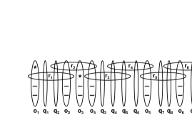
(a) An instance

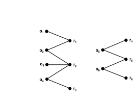
(b) The corresponding $H$

Figure 3: An example of an instance and the corresponding $H$ subgraph. In (a), the given instance is shown, where only the $4-$rows intersecting $O_{2,0}\cup O_{1,1}$ are included. A ’-’ stands for an uncovered base element, and a ’*’ stands for an element covered by a $3-$row. Thus, $o_{1},o_{3}\in O_{1,1}$, $o_{2},o_{4},o_{5},o_{6}\in O_{2,0}$, and $q_{1},...,q_{9}\notin O_{1,1}\cup O_{2,0}$. Also observe that $r_{1},r_{5}\in R_{\{2\}}^{H}$, $r_{3},r_{4},r_{6}\in R_{\{1\}}^{H}$, and $r_{2}\in R_{\{3\}}^{H}$.

Observe that $H$ need not be connected (as opposed to $G$, by Assumption 3.2). Also observe that since the only rows in $H$ are $4-$rows, each $O_{1,1}$ vertex has a single neighbor in $H$ (i.e., the $4-$row intersecting it). We record this fact for future reference:

Lemma 3.4

Each $O_{1,1}$ vertex is a leaf in $H$.

For any subgraph $F$ of $H$, let $\Delta(F)$ denote the maximum degree of a vertex in $F$. In addition, for $A\subseteq\{0,...,4\}$, let $R_{A}^{F}$ denote the set of row vertices in $F$ of degree $i$ in $F$ for some $i\in A$.

We start by investigating the number of $O_{1,1}$ vertices in $H$. The following result implies that there cannot be too many of them:

Lemma 3.5

Let $c,d$ be two distinct column vertices in $O_{1,1}$ which belong to the same CC of $H$. Then every $c-d$ path $P$ in $H$ has $n_{r}^{P}\geq\frac{1}{\epsilon}-1$ row vertices.

Proof: We may assume that $c$ and $d$ are connected by a (simple) path $P$ of minimum length among the paths in $H$ connecting a pair of $O_{1,1}$ vertices. Let $P\equiv(c,r_{1},c_{1},...,r_{l-1},c_{l-1},r_{l},d)$. By Lemma 3.4, the $O_{1,1}$ vertices are leaves in $H$. Therefore, the vertices $c_{1},...,c_{l-1}$ are $O_{2,0}$ columns, and $r_{1},...,r_{l}$ are $4-$rows. Denote by $r$ and $s$ the $3-$row neighbors in $G$ of $c$ and $d$, respectively, and define $P^{\prime}\equiv(r,c,r_{1},c_{1},...,r_{l-1},c_{l-1},r_{l},d,s)$. Observe that $P^{\prime}$ cannot be a cycle: if $r=s$, then removing (the $3-$row) $r$ from $APX$, and inserting the two $3-$column subsets $c\setminus r_{1}$ (i.e., $c$’s two uncovered base elements and the singleton $c\cap r$) and $d\setminus r_{l}$ increases the objective function by $1$, which is a contradiction to $APX$ being a local optimum. Thus, $P^{\prime}$ is path from $r$ to $s$. If $n_{r}^{P^{\prime}}\leq\frac{1}{\epsilon}$, the algorithm can replace the rows $r,r_{1},...,r_{l},s$ with the columns $c,c_{1},...,c_{l-1},d$, again increasing its objective function, which is a contradiction. Thus, $n_{r}^{P^{\prime}}\geq\frac{1}{\epsilon}+1$, implying $n_{r}^{P}=n_{r}^{P^{\prime}}-2\geq\frac{1}{\epsilon}-1$.    

Corollary 3.1

Every small CC of $H$ has at most one $O_{1,1}$ vertex.

As for big CCs, we have:

Lemma 3.6

Let $F$ be a big CC of $H$. Then $|O_{1,1}^{F}|=O(\epsilon)n_{r}^{F}$.

Proof: Assume that $|O_{1,1}^{F}|>1$, otherwise the claim is trivial. Construct a Voronoi diagram on the set of $F$’s vertices, with centers being its $O_{1,1}$ columns. By Lemma 3.5, any path connecting two distinct such centers has at least $\frac{1}{\epsilon}-1$ row vertices. Therefore, each Voronoi cell contains at least $\lfloor\frac{1}{2}(\frac{1}{\epsilon}-1)\rfloor$ vertices. Thus, $n_{r}^{F}\geq|O_{1,1}^{F}|\lfloor\frac{1}{2}(\frac{1}{\epsilon}-1)\rfloor$, implying $|O_{1,1}^{F}|=O(\epsilon)n_{r}^{F}$.    

Thus, the $O_{1,1}$ vertices are ”negligible” in $H$, both in small and big components. We proceed to investigate the number of $O_{2,0}$ vertices. We specify two useful properties of $H$: the first states that small CCs are either double edges (i.e., two parallel edges between a pair of vertices), cycles, or trees, and the second is a characterization of a local optimum.

Lemma 3.7

Every small CC of $H$ is either a double edge, a cycle, or a tree.

Proof: We prove the claim by showing that a small CC of $H$ cannot include a double edge or a cycle as a proper subset. Thus, any small CC which is not a double edge or a cycle must be a tree.

We start by showing that two vertices that are connected by a double edge have no other neighbors in $H$, implying that a CC of $H$ cannot include a double edge as a proper subset. Suppose that a column $c$ and a row $r$ are connected by a double edge. Since, by Lemma 3.4, the $O_{1,1}$ vertices are leaves, it follows that $c\in O_{2,0}$. Thus, $|r\cap c|=2$ (i.e., $r$ covers two base elements of $c$), and $c$ has no neighbors other than $r$. So suppose to the contrary that $r$ has an additional neighbor $d\neq c$. If $r$ covers two elements of $d$, then replacing $r$ with $c,d$ produces a better solution, which is a contraction. Otherwise, $|r\cap d|=1$ and $d$ has an additional neighbor, which we denote by $s$. Then removing $r$ and inserting $c$ and $d\setminus(d\cap s)$ (i.e., the $3$-row subset of $d$ consisting of $d$’s two uncovered elements and the singleton $r\cap d$) again produces a better solution, which is a contradiction.

In order to complete the proof, we show that a small cycle has no neighbors outside it, again, implying that a CC of $H$ cannot include it as a proper subset. Let $C$ be a small cycle in $H$. We show that for each vertex in $C$, its neighbors in $H$ are precisely its two neighbors in $C$. Again, since $O_{1,1}$ vertices are leaves (by Lemma 3.4), it follows that $C$’s vertices alternate between rows and $O_{2,0}$-columns. By definition, each $O_{2,0}$ column has exactly two $(4-)$row neighbors, hence, they are in $C$. As for the rows of $C$, suppose to the contrary that there exists a $(4-)$row vertex $r\in C$ that has a neighbor $c\in H\setminus C$. First observe that $r$ cannot be connected to $c$ by a double edge since in that case, as we just proved, that double edge is by itself a CC, which is a contradiction. Thus $r$ covers a single base element of $c$. Let $c^{\prime}$ be the $3-$column subset of $c$ consisting of $c$’s two uncovered base elements and (the singleton) $r\cap c$. As $n_{r}^{C}\leq\frac{1}{\epsilon}$, the following local step can be applied: remove $C$’s rows from the current solution and insert $C$’s columns and $c^{\prime}$. The number of $4-$sets in the new solution is the same, while the number of $3-$sets increases by one. Thus, this step is a local improvement one, which is a contradiction.    

Lemma 3.8

Let $T$ be a small subtree of $H$. (i) If all the leaves in $T$ are $(4-)$row vertices, then their number, $|R_{\{1\}}^{T}|$, is at most $4$. (ii) If $T$ has exactly $|R_{\{1\}}^{T}|=4$ leaves, then $T$ contains no $O_{1,1}$ vertices.

Proof: Assume $\Delta(T)>2$, otherwise the claim is trivial (note that for part (ii), if $\Delta(T)\leq 2$ then $T$ cannot have $4$ leaves). Hence $R_{\{3,4\}}^{T}\neq\emptyset$.
(i) Since $T$’s vertices alternate between rows and columns, it follows that

$$n_{r}^{T}=n_{c}^{T}+1\ .$$ (16)

To see this, partition $T$ into edge-disjoint paths by the following iterative procedure: start with any path $P$ connecting two arbitrary leaves, and mark its vertices. Clearly, $n_{r}^{P}=n_{c}^{P}+1$. As long as there exist unmarked vertices, choose a minimal (with respect to inclusion) path $Q$ connecting an unmarked leaf to a marked vertex $u$. Note that $u\in R_{\{3,4\}}^{T}$, i.e., $n_{r}^{Q}=n_{c}^{Q}+1$, and since $Q$ is minimal, all of $Q$’s vertices except for $u$ are unmarked. Marking $Q$’s vertices, the number of row vertices which are marked for the first time is equal to the number of such column vertices. Summing over all paths, we obtain $n_{r}^{T}=n_{c}^{T}+1$.

Observe that for each row leaf $r\in R_{\{1\}}^{T}$, $r$’s neighbor is a column in $O_{2,0}$, since the $O_{1,1}$ are leaves (by Lemma 3.4) and $\Delta(T)>2$ by assumption. As $n_{r}^{T}\leq\frac{1}{\epsilon}$, the following local step can be applied:

• remove the $n_{r}^{T}$ rows of $T$ from the current solution,

• insert the $n_{c}^{T}$ columns of $T$,

• for each ($4-$row) leaf $r\in R_{\{1\}}^{T}$, insert its $3-$row subset consisting of the three elements which are not covered by $r$’s ($O_{2,0}$) neighbor in $T$.

Thus, we traded one $4-$row for $|R_{\{1\}}^{T}|$ $3-$sets. Due to our objective function, we must have $|R_{\{1\}}^{T}|\leq 4$, otherwise this step would be a local improvement one, which is a contradiction.

(ii) Suppose to the contrary that there exists a subtree $T\subseteq H$ with $|R_{\{1\}}^{T}|=4$ row leaves such that $O_{1,1}^{F}\neq\emptyset$. Denote these row leaves by $r_{1},...,r_{4}$, and let $c_{1},...,c_{4}$ be their corresponding neighbors. Observe that $c_{1},...,c_{4}\notin O_{1,1}$, since if $c_{i}\in O_{1,1}$ for some $i$, then by Lemma 3.4 it is a leaf, implying that $(r_{i},c_{i})$ is an isolated edge, contradicting the assumption that $T$ is a tree with four leaves. By Corollary 3.1, there is exactly one $O_{1,1}^{F}$ vertex, which we denote by $c$. Let $r$ be $c$’s $3-$row neighbor, and let $T^{\prime}\equiv(V(T)\cup\{r\},E(T)\cup\{(c,r)\})$. Thus, all the leaves in $T^{\prime}$ are row vertices. It then follows, by exactly the same argument in part (i), that $n_{r}^{T^{\prime}}=n_{c}^{T^{\prime}}+1$. Therefore, in $T$ we have: $n_{r}^{T}=n_{c}^{T}$. As $n_{r}^{T^{\prime}}\leq\frac{1}{\epsilon}$, we can remove the $n_{r}^{T}$ $4-$rows and (the $3-$row) $r$, and insert the $n_{c}^{T}$ columns and the four $3-$row subsets of the leaves: $r_{i}\setminus c_{i}$, $i=1,...,4$. The number of $4-$sets remain the same, while the number of $3-$sets increases by $3$, which is a contradiction.    

We emphasize that $T$ need not be a CC of $H$. It may be a proper subset of a CC. If $T$ is a CC, the following result holds:

Corollary 3.2

Let $T$ be a small CC of $H$ which is a tree. Then $|R_{\{1\}}^{T}|\leq 4$, $|R_{\{3,4\}}^{T}|\leq 2$. Consequently, $|R_{\{2\}}^{T}|\geq n_{r}^{T}-6$.

Proof: The leaves of $T$ are either $R_{\{1\}}^{T}$ or $O_{1,1}$ vertices. If all of them are $R_{\{1\}}^{T}$ vertices, then by Lemma 3.8 (i): $|R_{\{1\}}^{T}|\leq 4$. Otherwise, Corollary 3.1 implies that $T$ contains exactly one $O_{1,1}$ vertex. Deleting it from $T$, we obtain a subtree $T^{\prime}$ whose all leaves are the $R_{\{1\}}^{T^{\prime}}$ vertices. By Lemma 3.8 (i): $|R_{\{1\}}^{T}|=|R_{\{1\}}^{T^{\prime}}|\leq 4$.

For the second part, recall from Graph Theory that the number of leaves in a nontrivial connected graph $G$ with $n_{i}$ vertices of degree $i$, $i=1,...,\Delta(G)$, is bounded by:

$$n_{1}\leq 2+\sum_{i=3}^{\Delta(G)}(i-2)n_{i}\ .$$ (17)

(This follows from $\sum_{i=1}^{\Delta(G)}in_{i}=2|E(G)|\geq 2(|V(G)|-1)=2(\sum_{i=1}^{\Delta(G)}n_{i}-1)$). If $G$ is a tree, then (17) holds as an equality, which we apply to $T$ and obtain:

$$|R_{\{1\}}^{T}|=2+|R_{\{3\}}^{T}|+2|R_{\{4\}}^{T}|\ .$$ (18)

We then conclude that:

$$|R_{\{3,4\}}^{T}|=|R_{\{3\}}^{T}|+|R_{\{4\}}^{T}|\leq|R_{\{3\}}^{T}|+2|R_{\{4\}}^{T}|=|R_{\{1\}}^{T}|-2\leq 2\ .$$

(The last inequality follows from the first part). Thus $|R_{\{3,4\}}^{T}|\leq 2$.    

Corollary 3.2 implies that most of the rows in a small tree $T$ have degree $2$, i.e., they are the $R_{\{2\}}^{T}$ vertices. This is intuitive, as we can view these rows as ”links” connecting two columns in a ”chain”, while very few rows are ”end-rows” (namely, the $R_{\{1\}}^{T}$ ones), and even fewer rows are ”links” to other ”chains” (the $R_{\{3,4\}}^{T}$ ones). Observe that for $F$ a cycle or a double edge, it is trivial that all the rows have degree $2$, i.e. $|R_{\{1\}}^{F}|=|R_{\{3,4\}}^{F}|=0$, $|R_{\{2\}}^{F}|=n_{r}^{F}$.

For the big CCs of $H$, the dominance of the $R_{\{2\}}$ rows still holds, but in a weaker sense. In order to establish it, we look at small neighborhoods around the vertices of a big CC $F$, bound the number of vertices of degrees $3$ or $4$, and by summation obtain a bound on $|R_{\{3,4\}}^{F}|$. A bound on $|R_{\{1\}}^{F}|$ then follows naturally.

Definition 3.3

For $\epsilon>0$ and $v\in H$, let $B_{\epsilon}(v)$ be the neighborhood of radius $\frac{1}{5\epsilon}$ centered at $v$ in $H$, i.e., the set of all vertices $u$ in $H$ such there exists a $u-v$ path in $H$ of length at most $\frac{1}{5\epsilon}$.

Observe that $|B_{\epsilon}(v)|$ may be greater than $\frac{1}{\epsilon}$. In addition, it is possible for a ”boundary” vertex $u\in B_{\epsilon}(v)$ that $deg_{B_{\epsilon}(v)}(u)<deg_{H}(u)$, i.e., if its distance from $v$ is exactly $\frac{1}{5\epsilon}$.

Lemma 3.9

For any $v\in H$, $B_{\epsilon}(v)$ contains at most two vertices of degree $3$ or $4$ in $H$, i.e., $|B_{\epsilon}(v)\cap R_{\{3,4\}}^{H}|\leq 2$.

Proof: Suppose to the contrary that there exists $v\in H$ such that $B_{\epsilon}(v)$ contains at least $3$ vertices in $R_{\{3,4\}}^{H}$. Pick any three of these vertices and denote them by $v_{1},v_{2},v_{3}$. Let $B^{\prime}$ be a spanning tree of $B_{\epsilon}(v)$, and let $P_{i}$ be the $v-v_{i}$ path in $B^{\prime}$, $i=1,2,3$. Let $T$ be the subtree of $B^{\prime}$ defined by $T\equiv\bigcup_{i=1}^{3}P_{i}$. We first show how to augment $T$ to obtain a subtree $T^{\prime}\subseteq B_{\epsilon}(v)$ with at least $5$ leaves which are column vertices:

• Case 1: $T$ has at least two leaves in $\{v_{1},v_{2},v_{3}\}$, say $v_{1}$ and $v_{2}$. Then each of $v_{1},v_{2}$ has at least two neighbors which are not in $T$, and in addition, either $v$ is a leaf or $v_{3}$ has at least one neighbor which is not in $T$. These neighbors are distinct and are different from $v$, otherwise $H$ contains a small cycle as a proper subset, contradicting Lemma 3.7. Let $T^{\prime}$ be the tree obtained by adding the edges connecting these neighbors to $T$. Then $T^{\prime}$ has at least $5$ leaves, which are columns.

• Case 2: $T$ is a simple path from $v$ to (say) $v_{1}$: then $v_{1}$ has at least two neighbors which are not in $T$, and each of $v_{2},v_{3}$ has at least one neighbor which is not in $T$. These neighbors are distinct by an argument similar to that in Case 1. Let $T^{\prime}$ be the tree obtained by adding the edges connecting these neighbors to $T$. Then again, $T^{\prime}$ has at least $5$ column leaves ($v$ being one of them).

In both cases, we obtained a tree $T^{\prime}$ of size at most $\frac{3}{5\epsilon}+5$, which we clearly may assume to be less than $\frac{1}{\epsilon}$, with at least $5$ leaves which are column vertices. Now, since $T^{\prime}$ is small, it follows by Corollary 3.1 that among these $5$ column leaves, at most one is an $O_{1,1}$ column vertex. Thus, at least $4$ leaves are $O_{2,0}$ columns. Each such $O_{2,0}$ leaf has an additional row neighbor outside $T^{\prime}$. Again, these neighbors are distinct, otherwise there is a contradiction to Lemma 3.7. Adding the edges connecting these row neighbors to $T^{\prime}$, we obtain a tree of size at most $\frac{3}{5\epsilon}+10\leq\frac{1}{\epsilon}$. It either has $5$ or more row leaves, or exactly $4$ row leaves and one $O_{1,1}$ leaf. In both cases we obtain a contradiction to Lemma 3.8.    

We are now ready to upper-bound the number of vertices of degree $1,3$, and $4$ in the big CCs of $H$. In particular, this establishes the dominance (in terms of a lower bound) of rows of degree $2$ which we previously stated. Since, as we mentioned, we look at each CC separately, all bounds are in terms of the total number of rows in the specific CC.

Lemma 3.10

Let $F$ be a big CC of $H$. (i) $|R_{\{3,4\}}^{F}|=O(\epsilon)n_{r}^{F}$, (ii) $|R_{\{1\}}^{F}|=O(\epsilon)n_{r}^{F}$, (iii) $|R_{\{2\}}^{F}|\geq(1-O(\epsilon))n_{r}^{F}$.

Proof: For part (i), observe that:

$$|R_{\{3,4\}}^{F}|=\sum_{v\in R_{\{3,4\}}^{F}}1\leq\sum_{v\in R_{\{3,4\}}^{F}}5\epsilon|B_{\epsilon}(v)|\ ,$$

where the inequality follows from the fact that for $v$ in a big CC, $|B_{\epsilon}(v)|\geq\frac{1}{5\epsilon}$.

Now, consider the multi-set of vertices which belong to the (possibly overlapping) neighborhoods around all of $R_{\{3,4\}}^{F}$ vertices, that is, we look at $S\equiv\cup_{v\in R_{\{3,4\}}^{F}}B_{\epsilon}(v)$ where we allow repetitions of elements in $S$. Every vertex appears at most twice in $S$. To see this, suppose to the contrary that there is a vertex $u$ which appears at least three times in $S$. Then any three centers of neighborhoods which cover $u$ are three $R_{\{3,4\}}^{F}$ vertices in $B_{\epsilon}(u)$. $F$ is a CC of $H$, therefore $R_{\{3,4\}}^{F}\subseteq R_{\{3,4\}}^{H}$, implying $|B_{\epsilon}(u)\cap R_{\{3,4\}}^{H}|\geq|B_{\epsilon}(u)\cap R_{\{3,4\}}^{F}|\geq 3$, which is a contradiction to Lemma 3.9. Hence, $\sum_{v\in R_{\{3,4\}}^{F}}|B_{\epsilon}(v)|=|S|\leq 2n_{F}$. Combining this with the previous inequality, we obtain:

$$|R_{\{3,4\}}^{F}|\leq 10\epsilon n_{F}\ .$$ (19)

We would like to obtain the bound in terms of $n_{r}^{F}$, the number of rows in $F$. Observe that each column intersects at most $4$ rows. Thus, $n_{c}^{F}\leq 4n_{r}^{F}$, implying that $n_{F}=n_{r}^{F}+n_{c}^{F}\leq 5n_{r}^{F}$. Substituting this in (19), we obtain:

$$|R_{\{3,4\}}^{F}|\leq 50\epsilon n_{r}^{F}\ .$$ (20)

This proves part (i).

For part (ii), applying (17) to $F$, we obtain:

$$|R_{\{1\}}^{F}|\leq 2+|R_{\{3\}}^{F}|+2|R_{\{4\}}^{F}|\leq 2+2|R_{\{3,4\}}^{F}|\leq 2+100\epsilon n_{r}^{F}\leq 102\epsilon n_{r}^{F}\ ,$$

where the third inequality follows from (20), and the last one from the assumption that $F$ is big. This proves part (ii).

Part (iii) follows from parts (i) and (ii) (as $n_{r}^{F}=|R_{\{1\}}^{F}|+|R_{\{2\}}^{F}|+|R_{\{3,4\}}^{F}|$). This completes the proof.    

Now consider the $O_{2,0}^{F}$ columns for some big CC $F$ of $H$. We show that their number is about the same as that of $R_{\{2\}}^{F}$ vertices. Intuitively, this is true since, as we proved, most of $F$’s columns are in $O_{2,0}^{F}$, most of its rows are in $R_{\{2\}}^{F}$, and in every path the vertices alternate between rows and columns. Formally:

Lemma 3.11

For a big CC $F$ of $H$: $|R_{\{2\}}^{F}|-O(\epsilon)n_{r}^{F}\leq|O_{2,0}^{F}|\leq|R_{\{2\}}^{F}|+O(\epsilon)n_{r}^{F}$.

Proof: Let $F$ be a big CC of $H$. We bound $\sum_{i=1}^{4}i|R_{\{i\}}^{F}|$ from below and from above to obtain:

$$2|R_{\{2\}}^{F}|\leq\sum_{i=1}^{4}i|R_{\{i\}}^{F}|\leq|R_{\{1\}}^{F}|+2|R_{\{2\}}^{F}|+4|R_{\{3,4\}}^{F}|\leq 2|R_{\{2\}}^{F}|+O(\epsilon)n_{r}^{F}\ ,$$

where the last inequality follows from Lemma 3.10(i),(ii). Counting $F$’s edges using each of its two partite sets, we obtain:

$$\sum_{i=1}^{4}i|R_{\{i\}}^{F}|=|O_{1,1}^{F}|+2|O_{2,0}^{F}|=2|O_{2,0}^{F}|+O(\epsilon)n_{r}^{F}\ ,$$

where the last equality is by Lemma 3.6. Thus:

$$2|R_{\{2\}}^{F}|\leq 2|O_{2,0}^{F}|+O(\epsilon)n_{r}^{F}\leq 2|R_{\{2\}}^{F}|+O(\epsilon)n_{r}^{F}\ .$$

Subtracting $O(\epsilon)n_{r}^{F}$ from all sides and dividing by $2$ yields the claim.
   

We note that for small CC’s, the last result holds in a stronger sense:

Remark 3.1

Let $F$ be a CC of $H$. (i) If $F$ is a small tree then $|R_{\{2\}}^{F}|-1\leq|O_{2,0}^{F}|\leq|R_{\{2\}}^{F}|+5$. (ii) If $F$ is a small cycle or a double edge then $|O_{2,0}^{F}|=|R_{\{2\}}^{F}|$.

Proof: (i) Let $F$ be a small CC of $H$ which is a tree. First suppose that $F$ contains no $O_{1,1}$ vertices, i.e., all of its leaves the $R_{\{1\}}^{F}$ vertices. Then equality (16) holds for $F$, i.e., $n_{r}^{F}=n_{c}^{F}+1$ (this is true by the argument used in the proof of Lemma 3.8 (i)). Thus, $|O_{2,0}^{F}|=n_{c}^{F}=n_{r}^{F}-1$. We now bound $|O_{2,0}^{F}|$ from above and from below:

$$|O_{2,0}^{F}|=n_{r}^{F}-1\leq|R_{\{2\}}^{F}|+5\ ,$$

where the inequality follows from Corollary 3.2, and trivially:

$$|O_{2,0}^{F}|=n_{r}^{F}-1\geq|R_{\{2\}}^{F}|-1\ .$$

Thus, $|R_{\{2\}}^{F}|-1\leq|O_{2,0}^{F}|\leq|R_{\{2\}}^{F}|+5$, as required.

If $O_{1,1}^{F}\neq\emptyset$ then by Corollary 3.1, $F$ contains exactly one $O_{1,1}$ vertex. We delete it from $F$ to obtain a tree, denoted $F^{\prime}$, with all its leaves being $R_{\{1\}}$ vertices. Thus, the last result holds for $F^{\prime}$, i.e., $|R_{\{2\}}^{F^{\prime}}|-1\leq|O_{2,0}^{F^{\prime}}|\leq|R_{\{2\}}^{F^{\prime}}|+5$. By observing that $O_{2,0}^{F}=O_{2,0}^{F^{\prime}}$ and $R_{\{2\}}^{F}=R_{\{2\}}^{F^{\prime}}$, we establish the result for $F$ as well.

(ii) This is trivial.    

Recall that our goal is to bound $X_{1,1}$ and $X_{2,0}$ - the proportions of $O_{1,1}$ and $O_{2,0}$ in $G$. So far we obtained a good estimation of their proportions in $H$: Corollary 3.1 and Lemma 3.6 imply that the $O_{1,1}$ vertices are negligible in small and big CCs of $H$, respectively ; Lemma 3.11 and Remark 3.1 imply that intuitively, the proportion of $O_{2,0}$ in $H$ is about one half (the other half consists mainly of rows of degree $2$). However, in order to bound the proportions in $G$, we need to take into account the columns which are not in $O_{1,1}$ or $O_{2,0}$ but intersect some row in that CC. This motivates the following construction:

The $\widetilde{H}$ graph
Denote those columns which intersect some row in $H$ and are not in $O_{1,1}\cup O_{2,0}$ by $\widetilde{O}$. We construct the $\widetilde{H}$ graph, which need not be a subgraph of $G$, in two steps. First, let $\widetilde{H}$ be the graph obtained from $H$ by connecting each row in $H$ to distinct new vertices representing the $\widetilde{O}$-columns intersecting it. We emphasize that an $\widetilde{O}$-column may appear in a few CCs of $\widetilde{H}$: Suppose $o\in\widetilde{O}$ and $C_{1},...,C_{l}$, $2\leq l\leq 4$ are CCs of $H$ such that each one contains a row intersecting $o$. Then each corresponding CC in $\widetilde{H}$ will have its own (distinct) vertex representing $o$. Thus, in terms of vertex labels (where each vertex has a label of the set represented by it), the CCs of $\widetilde{H}$ are not $\widetilde{O}$-column-disjoint. But they are $O_{1,1}\cup O_{2,0}$-column-disjoint as well as row-disjoint, and hence in particular are edge-disjoint. Figure 4 shows the $\widetilde{H}$ graph corresponding to the instance given in Figure 3 up to this step.

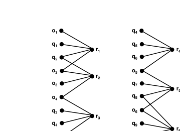
Figure 4: The $\widetilde{H}$ graph corresponding to the instance given in Figure 3 prior to the addition of the $\widetilde{H}_{0}$ subgraph.

At a final step in the construction, we add to $\widetilde{H}$ the subgraph of $G$ induced by the set of remaining vertices (if any), that is, all vertices which do not belong to any CC from the previous step. Denote this subgraph by $\widetilde{H}_{0}$. Note that $\widetilde{H}_{0}$ need not be connected. Let $\mathcal{C}$ denote the collection of $\widetilde{H}$’s CCs. The disjointness of the rows implies:

$$n_{r}=n^{\widetilde{H}}_{r}=\sum_{F\in\mathcal{C}\cup\widetilde{H}_{0}}n^{F}_{r}\ .$$ (21)

We use the following notation. Let $F\in\mathcal{C}\cup\widetilde{H}_{0}$. Denote by $\widetilde{O}^{F}$ the $\widetilde{O}$-columns in $F$. Denote by $E_{2,0}^{F}$ the set of edges incident to the $O_{2,0}^{F}$ columns, by $E_{1,1}^{F}$ the set of edges incident to the $O_{1,1}^{F}$ columns, and by $\widetilde{E}^{F}$ the set of remaining edges, i.e. $\widetilde{E}^{F}\equiv E(F)\setminus(E_{2,0}^{F}\cup E_{1,1}^{F})$. Note that for $F\in\mathcal{C}$ ($F\neq\widetilde{H}_{0}$), all the edges in $\widetilde{E}^{F}$ are incident to columns in $\widetilde{O}^{F}$. Define $E_{2,0}\equiv\bigcup_{F\in\mathcal{C}}\widetilde{E}_{2,0}^{F}$, $E_{1,1}\equiv\bigcup_{F\in\mathcal{C}}\widetilde{E}_{1,1}^{F}$, and $\widetilde{E}\equiv\bigcup_{F\in\mathcal{C}}\widetilde{E}^{F}$. Finally, denote by $r_{i}^{F}$ the number of rows in $V(F)\cap R_{\{i\}}^{H}$. The following observations are trivial (the first two hold in $H$ as well):

Lemma 3.12

(i) For each $F\in\mathcal{C}\cup\widetilde{H}_{0}$, $|E_{1,1}^{F}|=|O_{1,1}^{F}|$ and $|E_{2,0}^{F}|=2|O_{2,0}^{F}|$, (ii) For each $F\in\mathcal{C}$, each vertex $o\in O_{1,1}^{F}$ is a leaf in $F$, (iii) For each $F\in\mathcal{C}$, a row in $F$ which belongs to $R_{\{i\}}^{H}$ contributes $i$ edges to $E_{1,1}^{F}\cup E_{2,0}^{F}$ and $4-i$ edges to $\widetilde{E}^{F}$, $i=1,...,4$, that is:

$$|E_{2,0}^{F}|+|E_{1,1}^{F}| = r_{1}^{F}+2r_{2}^{F}+3r_{3}^{F}+4r_{4}^{F}\ ,$$ (22)

$$|\widetilde{E}^{F}| = 3r_{1}^{F}+2r_{2}^{F}+r_{3}^{F}\ .$$ (23)

Lemma 3.13

For any Type A-instance,

$$|\widetilde{E}|\leq|O_{1,2}|+|O_{1,3}|+2|O_{2,1}|+2|O_{2,2}|+3|O_{3,0}|+3|O_{3,1}|+4|O_{4,0}|\ .$$ (24)

Proof: Consider a vertex $o\in O_{i,j}$, $i\geq 1$, $(i,j)\notin\{(1,1),(2,0)\}$. $o\in\widetilde{O}$ if there exist an $O_{2,0}$-column $q$ and a $4-$row $r$ such that $r\cap q\neq\emptyset$ and $r\cap o\neq\emptyset$. In this case, $o$ contributes at most $i$ edges (possibly in different CCs) to $\widetilde{E}$. (Otherwise it contributes zero).    

We now derive a linear inequality, which provides an upper-bound on the number of edges in $E_{2,0}$ and $E_{1,1}$.

Lemma 3.14

For any Type A-instance, $|E_{2,0}|+3|E_{1,1}|\leq|\widetilde{E}|+O(\epsilon)n_{r}$.

Proof: We show that for every $F\in\mathcal{C}\cup\widetilde{H}_{0}$, we have:

$$|E_{2,0}^{F}|+3|E_{1,1}^{F}|\leq|\widetilde{E}^{F}|+O(\epsilon)n^{F}_{r}\ .$$ (25)

By definitions of $E_{2,0}$, $E_{1,1}$ and $\widetilde{E}$, and using (21), the claim then follows by summing over all $F\in\mathcal{C}\cup\widetilde{H}_{0}$. We distinguish four cases, according to the type of $F$.

• Case 1: $F=\widetilde{H}_{0}$
  Since $\widetilde{H}_{0}$ contains no $O_{1,1}$ and $O_{2,0}$ vertices, it follows that $E_{1,1}^{\widetilde{H}_{0}}=E_{2,0}^{\widetilde{H}_{0}}=\emptyset$. Hence (25) trivially holds.

• Case 2: $F$ is a CC of $\widetilde{H}$ obtained from a double edge or a small cycle in $H$
  Denote by $C$ the double edge or the cycle in $H$ from which $F$ is obtained. Then $C$ is a CC of $H$, and its rows are precisely the rows of $F$ (because $\widetilde{H}$ was obtained from $H$ by adding columns). $C$ has even length, with its vertices alternating between $O_{2,0}$ columns and $R_{\{2\}}^{H}$ $(4-)$rows. Thus, each such row has two $O_{2,0}$ column neighbors (in $C$ and therefore in $F$) and two $\widetilde{O}$ column neighbors (in $F\setminus C$). Therefore, it contributes two edges to $E_{2,0}^{F}$ and two to $\widetilde{E}^{F}$, i.e.:

  $$|E_{2,0}^{F}|=|\widetilde{E}^{F}|=2n_{r}^{F}\ .$$ (26)

  Finally, observe that $O_{1,1}^{F}=\emptyset$: this is true because as we just noted, $C$’s columns are only in $O_{2,0}$, and $F$ was obtained from $C$ by adding $\widetilde{O}$ columns (which, by definition, are not in $O_{1,1}$). Thus, $|O_{1,1}^{F}|=0$, implying that $|E_{1,1}|=0$. This fact and (26) establish (25).

• Case 3: $F$ is a CC of $\widetilde{H}$ obtained from a small tree in $H$
  The rows of $F$ are precisely the rows of the tree in $H$ which $F$ is obtained from. Thus, subtracting (22) from (23), we obtain:

  $$|\widetilde{E}^{F}|-|E_{2,0}^{F}|-|E_{1,1}^{F}|=2(r_{1}^{F}-r_{3}^{F}-2r_{4}^{F})=4\ ,$$

  where the last equality follows from $r_{1}^{F}=2+r_{3}^{F}+2r_{4}^{F}$, which holds due to (18). This implies:

  $$|E_{2,0}^{F}|\leq|\widetilde{E}^{F}|-4\ .$$ (27)

  Now, by Corollary 3.1, $F$ can have at most one $O_{1,1}$ vertex. By Lemma 3.12 (ii), such a vertex is a leaf in $F$, implying that $|E_{1,1}^{F}|=|O_{1,1}^{F}|\leq 1$. Combining this with (27), we obtain:

  $$|E_{2,0}^{F}|+3|E_{1,1}^{F}|\leq|E_{2,0}^{F}|+3\leq|\widetilde{E}^{F}|-1\ ,$$

  establishing (25).

• Case 4: $F$ is a CC of $\widetilde{H}$ obtained from a big CC of $H$
  We have:

  $$|\widetilde{E}^{F}|\geq 2r_{2}^{F}\geq 2|O_{2,0}^{F}|-O(\epsilon)n_{r}^{F}=|E_{2,0}^{F}|-O(\epsilon)n_{r}^{F}\ ,$$

  where the first inequality follows from (23), the second inequality follows from Lemma 3.11, and the equality follows from Lemma 3.12 (i). In order to complete the proof, it suffices to show that $|E_{1,1}^{F}|=O(\epsilon)n_{r}^{F}$. Denote by $F^{\prime}$ the (big) CC of $H$ from which $F$ is obtained. By Lemma 3.6, we have $|O_{1,1}^{F^{\prime}}|=O(\epsilon)n_{r}^{F^{\prime}}$. Since $O_{1,1}^{F^{\prime}}=O_{1,1}^{F}$ and similarly, the rows of $F^{\prime}$ are precisely the rows of $F$, we also have: $|O_{1,1}^{F}|=O(\epsilon)n_{r}^{F}$. By Lemma 3.12 (i): $|E_{1,1}^{F}|=|O_{1,1}^{F}|$. Hence $|E_{1,1}^{F}|=O(\epsilon)n_{r}^{F}$, as required.

 

We are now ready to bound a linear combination of $X_{2,0}$ and $X_{1,1}$:

Lemma 3.15

For any Type A-instance:

$$2X_{2,0}+3X_{1,1}\leq X_{1,2}+X_{1,3}+2X_{2,1}+2X_{2,2}+3X_{3,0}+3X_{3,1}+4X_{4,0}+O(\epsilon)\ .$$ (28)

Proof: From Lemma 3.14 we have: $|E_{2,0}|+3|E_{1,1}|\leq|\widetilde{E}|+O(\epsilon)n_{r}$. From Observation 3.1 we obtain $n_{r}=\Theta(n_{c})$, so we also have: $|E_{2,0}|+3|E_{1,1}|\leq|\widetilde{E}|+O(\epsilon)n_{c}$. We would like to write this inequality in terms of the column sets. By summation, Lemma 3.12(i) implies that $|E_{1,1}|=|O_{1,1}|$ and $|E_{2,0}|=2|O_{2,0}|$. Thus, we obtain:

$$2|O_{2,0}|+3|O_{1,1}|\leq|\widetilde{E}|+O(\epsilon)n_{c}\ .$$ (29)

Using Lemma 3.13, we obtain:

$$2|O_{2,0}|+3|O_{1,1}|\leq|O_{1,2}|+|O_{1,3}|+2|O_{2,1}|+2|O_{2,2}|+3|O_{3,0}|+3|O_{3,1}|+4|O_{4,0}|+O(\epsilon)n_{c}\ .$$

Dividing both sides by $n_{c}=|OPT|$, we obtain the required inequality.    

By providing the last constraint, Lemma 3.15 concludes our construction of the LP, which upper-bounds $\rho$ - the approximation ratio of the algorithm (for Type A-instances). Recall that the other constraints are that the variables are non-negative and that their sum is $1$. In addition, the variables $X_{0,0},X_{0,1},X_{0,2},X_{0,3},X_{1,0}$ are zero, by Lemma 3.2. The objective function was stated in (15). Thus, the complete program is:

$$\max \sum_{0\leq i+j\leq 4}c_{i,j}X_{i,j}\qquad\qquad\qquad\qquad\qquad\qquad\qquad\qquad\qquad\qquad$$

s.t. $$3X_{1,1}-X_{1,2}-X_{1,3}+2X_{2,0}-2X_{2,1}-2X_{2,2}-3X_{3,0}-3X_{3,1}-4X_{4,0}\leq O(\epsilon)$$

$$\sum_{0\leq i+j\leq 4}X_{i,j}=1\qquad\qquad\qquad\qquad\qquad\qquad\qquad\qquad\qquad\qquad\qquad$$

$$X_{i,j}\geq 0\qquad\qquad 0\leq i+j\leq 4\qquad\qquad\qquad\qquad\qquad\qquad\qquad\quad$$

$$X_{0,0},X_{0,1},X_{0,2},X_{0,3},X_{1,0}=0\qquad\qquad\qquad\qquad\qquad\qquad\qquad\qquad\quad$$

(inequality (3.2) is obtained from (28) by rearranging terms). Specifically, given $\epsilon>0$, the ratio $\rho$ is upper-bounded by the objective function value of the LP. We now turn to solve this program. We simplify it, first by omitting the zero variables $X_{0,0},X_{0,1},X_{0,2},X_{0,3},X_{1,0}$. Denote the set of (remaining) relevant indices by $I\equiv\{(1,1),(1,2),(1,3),(2,0),(2,1),(2,2),(3,0),(3,1),(4,0)\}$. Next, since our goal is to solve the LP for arbitrarily small values of $\epsilon$, we replace $O(\epsilon)$ in the constraint (3.2) by zero. Using (14) to obtain the explicit values of $c_{i,j}$’s, the modified LP is:

$$\max \frac{19}{12}X_{1,1}+\frac{17}{12}X_{1,2}+\frac{5}{4}X_{1,3}+\frac{3}{2}X_{2,0}+\frac{4}{3}X_{2,1}+\frac{7}{6}X_{2,2}+\frac{5}{4}X_{3,0}+\frac{13}{12}X_{3,1}+X_{4,0}$$

s.t. $$3X_{1,1}-X_{1,2}-X_{1,3}+2X_{2,0}-2X_{2,1}-2X_{2,2}-3X_{3,0}-3X_{3,1}-4X_{4,0}\leq 0$$ (31)

$$\sum_{(i,j)\in I}X_{i,j}=1\qquad\qquad\qquad\qquad\qquad\qquad\qquad\qquad\qquad\qquad\qquad$$

$$X_{i,j}\geq 0\qquad\qquad(i,j)\in I\qquad\qquad\qquad\qquad\qquad\qquad\qquad\quad$$

In order to solve this LP, we use the dual program. Let $y,z$ be the dual variables corresponding to constraints (31),(3.2), respectively. The dual program is then:

$$\min z\qquad\qquad\qquad\qquad\qquad\qquad$$

s.t. $$3y+z\geq\frac{19}{12}\qquad\qquad\qquad\quad$$

$$-y+z\geq\frac{17}{12}\qquad\qquad\qquad\quad$$

$$-y+z\geq\frac{5}{4}\qquad\qquad\qquad\quad$$

$$2y+z\geq\frac{3}{2}\qquad\qquad\qquad\quad$$

$$-2y+z\geq\frac{4}{3}\qquad\qquad\qquad\quad$$

$$-2y+z\geq\frac{7}{6}\qquad\qquad\qquad\quad$$

$$-3y+z\geq\frac{5}{4}\qquad\qquad\qquad\quad$$

$$-3y+z\geq\frac{13}{12}\qquad\qquad\qquad\quad$$

$$-4y+z\geq 1\qquad\qquad\qquad\quad$$

$$y\geq 0\qquad\qquad\qquad\quad$$

Let $X^{*}$ be the vector consisting of $X_{1,1}=\frac{1}{4},X_{1,2}=\frac{3}{4}$, and $X_{i,j}=0$ for all $(i,j)\in I\setminus\{(1,1),(1,2)\}$. It is clear that $X^{*}$ is a feasible primal solution. The corresponding objective function value is $c_{1,1}X_{1,1}^{*}+c_{1,2}X_{1,2}^{*}=\frac{19}{12}\cdot\frac{1}{4}+\frac{17}{12}\cdot\frac{3}{4}=\frac{35}{24}$. Let $(y^{*},z^{*})\equiv(\frac{1}{24},\frac{35}{24})$. It is straightforward to verify that it is a feasible dual solution. The corresponding objective function value is $z^{*}=\frac{35}{24}$, which is equal to that of the primal. Thus, from the duality theorem, we conclude that $X^{*}$ and $(y^{*},z^{*})$ are optimal solutions to the primal and dual programs, respectively. By the construction of the (primal) LP, we conclude the following result:

Theorem 3.1

For Type A-instances, $A2$ is a $(\rho+\epsilon)$-approximation algorithm for $(2,4)$-UUSC, where $\rho\leq\frac{35}{24}=1.458333...$

3.3 Bounding $\rho$ in Type B-instances

In this subsection we assume that the instance is of Type B, that is, $OPT$ consists of $3-$ and $4-$columns, and $APX$ consists of $2-$ and $4-$rows. We use the analogous notation to that of the previous section.

Definition 3.4

For given $OPT$ and $APX$, let $O_{i}^{4}$ be the set of $4-$columns in which $i$ elements are covered (by $4-$rows), $i=0,...,4$, and let $X_{i}^{4}\equiv\frac{|O_{i}^{4}|}{|OPT|}$ be the proportion of these columns in $OPT$. Similarly, let $O_{i}^{3}$ be the set of $3-$columns in which $i$ elements are covered (by $4-$rows), $i=0,...,3$, and let $X_{i}^{3}\equiv\frac{|O_{i}^{3}|}{|OPT|}$. For any graph $F$, let $O_{i}^{s,F}\equiv O_{i}^{s}\cap V(F)$, $s=3,4$, $i=0,...,s$.

The objective function of set cover in terms of these new variables is:

$$|APX|=X_{2}+X_{3}+X_{4}=\sum_{i=0}^{4}c_{i}^{4}|O_{i}^{4}|+\sum_{i=0}^{3}c_{i}^{3}|O_{i}^{3}|$$ (33)

where

$$c_{i}^{4}\equiv\frac{i}{4}+\frac{4-i}{2}=2-\frac{i}{4}\ ,\qquad i=0,...,4\ ,$$

and

$$c_{i}^{3}\equiv\frac{i}{4}+\frac{3-i}{2}=\frac{3}{2}-\frac{i}{4}\ ,\qquad i=0,...,3\ .$$

Explicitly, the column costs are:

$$(c_{0}^{4},...,c_{4}^{4})=(2,1.75,1.5,1.25,1)\quad,\quad(c_{0}^{3},...,c_{3}^{3})=(1.5,1.25,1,0.75)\ .$$ (34)

Observe that $c_{i}^{4}=c_{i,0}$ from the previous section ($i=0,...,4$). The objective function of our LP, which bounds $\rho$ from above, is:

$$\max\sum_{i=0}^{4}c_{i}^{4}X_{i}^{4}+\sum_{i=0}^{3}c_{i}^{3}X_{i}^{3}\ .$$ (35)

Considering the highest $c_{i}^{j}$’s (i.e., the costs of the most expensive columns), the following result is analogous to Lemma 3.2 and therefore its proof is omitted:

Lemma 3.16

For any Type B-instance, $O_{0}^{3},O_{0}^{4},O_{1}^{4}=\emptyset$. Equivalently, $X_{0}^{3},X_{0}^{4},X_{1}^{4}=0$.

The next highest coefficient is $c_{2}^{4}=1.5$, so we derive a bound on $X_{2}^{4}$. The intersection graph $G$ is defined exactly the same, and we assume that it is connected and big (i.e., Assumption 3.2 holds for this instance type as well). Formally, it consists of $3-$ and $4-$columns in the $OPT$ partite, and $4-$rows in the $APX$ one. As for $H$ and $\widetilde{H}$:

The $H$ subgraph
$H$ is the subgraph of $G$ induced by the $O_{2}^{4}$-columns and the ($4-$)rows intersecting them. Note that these columns are analogous to the $O_{2,0}$ columns of Type A-instance, while there is no analog to $O_{1,1}$ columns. Thus, $H$’s structure is the same, that is, $H$ obtained from a Type B-instance is a special case of $H$ obtained from a Type A-instance, with no $O_{1,1}$ columns. Thus, the results from the previous section hold trivially. Specifically, regarding the $H$ subgraph, Lemmas 3.4, 3.5 and 3.6 are irrelevant, Lemma 3.7 holds, Lemma 3.8 (i) holds (part (ii) is irrelevant), Lemma 3.9 holds, and Lemma 3.10 holds. The analog of Lemma 3.11 is:

Lemma 3.17

For any Type B-instance, for each big CC F: $|R_{\{2\}}^{F}|-O(\epsilon)n_{r}^{F}\leq|O_{2}^{4,F}|\leq|R_{\{2\}}^{F}|+O(\epsilon)n_{r}^{F}.$

The $\widetilde{H}$ graph
$\widetilde{H}$ is, again, similar to $\widetilde{H}$ from the previous section, but with no columns analogous to $O_{1,1}$. Specifically, let $\widetilde{O}$ be the set of columns which intersect some row in $H$ (i.e., a $4-$row intersecting some $O_{2}^{4}$ column). For each CC $F$ of $H$, connect each row in $F$ to distinct vertices representing the $\widetilde{O}$-columns intersecting it. Denote these vertices by $\widetilde{O}^{F}$. Let $\widetilde{E}$ be the set new edges used to connect those vertices. Also, let $\widetilde{H}_{0}$ denote the subgraph of $G$ induced by the remaining vertices (which include all the $3-$rows), and add it to $\widetilde{H}$. Finally, let $E_{2}^{4,F}$, $\widetilde{E}^{F}$, $E_{2}^{4}$ denote the set of edges incident to $O_{2}^{4,F}$, $\widetilde{O}^{F}$, $O_{2}^{4}$ vertices, respectively. The analog of Lemma 3.12 is (only parts (i) and (iii) are relevant):

Lemma 3.18

(i) For each $F\in\mathcal{C}\cup\widetilde{H}_{0}$,

$$|E_{2}^{4,F}|=2|O_{2}^{4,F}|\ ,$$ (36)

(ii) For each $F\in\mathcal{C}$, a row in $F$ which belongs to $R_{\{i\}}^{H}$ contributes $i$ edges to $E_{2}^{4,F}$ and $4-i$ edges to $\widetilde{E}^{F}$, $i=1,...,4$.

The analogs of Lemmas 3.13 and 3.14 are, respectively:

Lemma 3.19

For any Type B-instance,

$$|\widetilde{E}|\leq|O_{1}^{3}|+2|O_{2}^{3}|+3|O_{3}^{4}|+3|O_{3}^{3}|+4|O_{4}^{4}|\ ,$$ (37)

Lemma 3.20

For any Type B-instance,

$$|E_{2}^{4}|\leq|\widetilde{E}|+O(\epsilon)n_{r}\ .$$ (38)

(The proof of Lemma 3.20 is identical to that of Lemma 3.14 with substituting $E_{2}^{4,F}$ for $E_{2,0}^{F}$ and $\emptyset$ for $E_{1,1}^{F}$).

Using (36) and summing over all $F\in\mathcal{C}\cup\widetilde{H}_{0}$, we obtain:

$$|E_{2}^{4}|=\sum_{F\in\mathcal{C}\cup\widetilde{H}_{0}}|E_{2}^{4,F}|=\sum_{F\in\mathcal{C}\cup\widetilde{H}_{0}}2|O_{2}^{4,F}|=2|O_{2}^{4}|\ .$$ (39)

Now, substituting (39) in the left-hand side of (38), and (37) in its right-hand side, and using $n_{r}=\Theta(n_{c})$ (from Observation 3.1), we obtain:

$$2|O_{2}^{4}|\leq|O_{1}^{3}|+2|O_{2}^{3}|+3|O_{3}^{4}|+3|O_{3}^{3}|+4|O_{4}^{4}|+O(\epsilon)n_{c}\ .$$

Dividing by $n_{c}=|OPT|$, we obtain the analog of Lemma 3.15:

Lemma 3.21

For any Type B-instance:

$$2X_{2}^{4}\leq X_{1}^{3}+2X_{2}^{3}+3X_{3}^{4}+3X_{3}^{3}+4X_{4}^{4}+O(\epsilon)n_{c}\ .$$

Using (34), the inequality from Lemma 3.21, and substituting $X_{0}^{3},X_{0}^{4},X_{1}^{4}=0$ (by Lemma 3.16), we obtain the following LP, which upper-bounds $\rho$ for Type B-instances:

$$\max 1.5X_{2}^{4}+1.25X_{3}^{4}+X_{4}^{4}+1.25X_{1}^{3}+X_{2}^{3}+0.75X_{3}^{3}$$

s.t. $$2X_{2}^{4}-3X_{3}^{4}-4X_{4}^{4}-X_{1}^{3}-2X_{2}^{3}-3X_{3}^{3}\leq 0$$

$$X_{2}^{4}+X_{3}^{4}+X_{4}^{4}+X_{1}^{3}+X_{2}^{3}+X_{3}^{3}=1\qquad\quad$$

$$X_{2}^{4},X_{3}^{4},X_{4}^{4},X_{1}^{3},X_{2}^{3},X_{3}^{3}\geq 0\qquad\quad$$

The dual program is:

$$\min z\qquad\qquad\qquad\qquad\qquad\qquad$$

s.t. $$2y+z\geq 1.5\qquad\qquad\qquad\quad$$

$$-3y+z\geq 1.25\qquad\qquad\qquad\quad$$

$$-4y+z\geq 1\qquad\qquad\qquad\quad$$

$$-y+z\geq 1.25\qquad\qquad\qquad\quad$$

$$-2y+z\geq 1\qquad\qquad\qquad\quad$$

$$-3y+z\geq 0.75\qquad\qquad\qquad\quad$$

$$y\geq 0\qquad\qquad\qquad\quad$$

It is straightforward to verify that:

$$X^{*}\equiv(X_{2}^{4},X_{3}^{4},X_{4}^{4},X_{1}^{3},X_{2}^{3},X_{3}^{3})=(\frac{3}{5},\frac{2}{5},0,0,0,0)$$

and

$$(y^{*},z^{*})=(\frac{1}{20},\frac{7}{5})$$

are primal and dual feasible solutions, respectively, achieving the same objective function value of $\frac{7}{5}$. Thus, they are optimal solution, which implies:

Theorem 3.2

For Type B-instances, $A2$ is a $(\rho+\epsilon)$-approximation algorithm for $(2,4)$-UUSC, where $\rho\leq\frac{7}{5}=1.4$.

Combining Theorems 3.1 and 3.2, and using Assumption 3.1, altogether we obtain:

Theorem 3.3

$A2$ is a $(\rho+\epsilon)$-approximation algorithm for $(2,4)$-UUSC, where $\rho\leq\frac{35}{24}=1.458333...$ .

In the following, we provide an example for which $\rho=\frac{25}{18}=1.3888...$ . The instance is of Type A. Let $|OPT|=36m$ for any fixed $m$, that is, $OPT$ consists of $36m$ $4-$columns, denoted $O_{1},...,O_{36m}$, covering $n=144m$ base elements. The construction of a local optimum $APX$ is as follows. The $4-$rows in $APX$ consist of two sets: In the first one, for each $i=1,...,12m-1$, there is a $4-$row which intersects (i.e., covers a single element of) the four columns $O_{3i-2},...,O_{3i+1}$, and there is one additional $4-$row intersecting $O_{1},O_{36m-2},O_{36m-1},O_{36m}$. Thus, the first set contains $12m$ rows. In the second set, for each $i=1,...,3m$, there are two $4-$rows: one intersecting $O_{3i-1},O_{9m+3i-1},O_{18m+3i-1},O_{27m+3i-1}$, and another one intersecting $O_{3i},O_{9m+3i},O_{18m+3i},O_{27m+3i}$. Thus, the second set contains $6m$ rows, so the total number of $4-$rows in $APX$ is $X_{4}=18m$.

As for the $3-$rows in $APX$, for each $i=1,...,4m$, there is one $3-$row intersecting $O_{3i-1},O_{12m+3i-1},O_{24m+3i-1}$, and another one intersecting $O_{3i},O_{12m+3i},O_{24m+3i}$. Thus, the total number of $3-$rows is $X_{3}=8m$.

For a given $\epsilon>0$, taking $m$ large enough ensures that $APX$ is a local optimum. Using the pricing scheme, it is easily verified that the $12m$ columns: $O_{3i-2}$, $i=1,...,12m$, are in $O_{2,0}$, and the remaining $24m$ columns are in $O_{2,1}$. Hence $X_{2,0}=\frac{1}{3}$, $X_{2,1}=\frac{2}{3}$. The corresponding costs are, by (14), $c_{2,0}=\frac{3}{2}$, $c_{2,1}=\frac{4}{3}$. The obtained approximation ratio is therefore:

$$\rho=c_{2,0}X_{2,0}+c_{2,1}X_{2,1}=\frac{3}{2}\cdot\frac{1}{3}+\frac{4}{3}\cdot\frac{2}{3}=\frac{25}{18}.$$

4 Concluding remarks

In this paper we focused on a special case of the unweighted $k$-set cover problem. We proposed a new paradigm to approach instances of this problem, and we showed that it gives better results than the previous known algorithms for unweighted $k$-set cover. Our proof is for a restricted case in which the instance contains all the pairs of elements. The technical reason to consider this special case is that all previous known improvements over the greedy algorithm have a special treatment of singletons, which makes the algorithms and their analysis much more complicated. By neglecting this technical problem, we can concentrate on the way to handle the selection of large sets.

In this paper we showed that the non-oblivious local search methodology can outperform the other methods to approximate unweighted $k$-set cover, and we conjecture that this is the case for the generalized case and not only for $(2,4)$-uniform instances. We leave as major open problems the tuning of the parameters for the non-oblivious local search algorithm (i.e., the weights used in the objective function of the local search), as well as the analysis of the resulting algorithm for unweighted $k$-set cover.

Appendix A Proof of Theorem 2.1

We prove that the solution for $(P)$ stated in the theorem is optimal, and then compute its objective function value. In order to show optimality, we construct the dual program of $(P)$, denoted $(D)$, provide a feasible solution to it, and then use a complementary slackness argument. By the complementary slackness, we conclude that both solutions are optimal. Then, we compute the objective function value of the primal solution. We start by constructing $(D)$. The dual decision variables are:

• $\beta_{p+1},...,\beta_{k}$ - correspond to the set of constraints (8),

• $\beta_{p}$ - corresponds to constraint (9),

• $\gamma_{p+1},...,\gamma_{k}$ - correspond to the set of constraints (2).

The dual program is:

Program $(D)$

$$\min \sum_{i=p}^{k}\beta_{i}\qquad\qquad\qquad\qquad\qquad$$

s.t. $$\beta_{k}-j\gamma_{k}\geq\frac{j}{k}\qquad\qquad\qquad\quad j=1,...,k-1$$ (40)

$$\beta_{k}-(k-2)\gamma_{k}\geq 1\qquad\qquad\quad$$ (41)

$$\beta_{i}-j\gamma_{i}+j\gamma_{i+1}\geq\frac{j}{i(i+1)}\qquad i=p+1,...,k-1,\quad j=1,...,i-1$$ (42)

$$\beta_{i}-(i-2)\gamma_{i}+i\gamma_{i+1}\geq\frac{1}{i+1}\quad i=p+1,...,k-1$$ (43)

$$\beta_{p}+p\gamma_{p+1}\geq\frac{1}{p+1}\quad\qquad\qquad$$

$$\beta_{i},\gamma_{j}\geq 0\qquad\qquad\qquad\qquad\quad i=p,...,k,\quad j=p+1,...,k\ .$$

For this LP, the primal variables $a_{k,1},...,a_{k,k-1}$ correspond to the set of constraints (40). $a_{k,k}$ corresponds to (41). $a_{i,j}$, $i=p+1,...,k-1$, $j=1,...,i-1$ correspond to (42). $a_{i,i}$, $i=p+1,...,k-1$ correspond to (43), and $a_{p,p}$ corresponds to (A).

The dual solution is the following (it is the same for the two cases distinguished in $(P)$, depending on the parity of $k-p$):

$$\begin{array}[]{llll}\gamma_{k}&=&\frac{1}{k(k-1)}&\\ \gamma_{k-1}&=&0&\\ \gamma_{i}&=&\gamma_{i+2}+\frac{2}{i(i+1)(i+2)}\ ,&\textrm{for all }i=p+1,...,k-2\\ \beta_{k}&=&1+(k-2)\gamma_{k}&\\ \beta_{i}&=&\frac{1}{i+1}-i\gamma_{i+1}+(i-2)\gamma_{i}\ ,&\textrm{for all }i=p+2,...,k-1\\ \beta_{p+1}&=&\frac{p}{(p+1)(p+2)}+p\gamma_{p+1}-p\gamma_{p+2}&\\ \beta_{p}&=&\frac{1}{p+1}-p\gamma_{p+1}\ .&\end{array}$$ (45)

We proceed to verify that the primal and dual solutions which we constructed are indeed feasible. In addition, we identify the set of tight constraints.

Lemma A.1

(Primal Feasibility)
The primal solution stated in Theorem 2.1 is feasible for $(P)$. Moreover, the set of constraints (8),(9) and (2) are tight, except for (2) for the value of $i=k-1$ when $k-p$ is odd.

Proof: First, it is trivial that the non-negativity constraints are satisfied since our solution is $0/1$. The set of constraints (8) are satisfied, and tight, since for each $i=p+1,...,k$, there exists exactly one $j$ index such that $a_{i,j}=1$ and for all other $j$ values $a_{i,j}=0$. Similarly, the constraint (9) is tight, as $a_{p,p}=1$. As for the set of constraints (2), which for convenience we rewrite as:

$$\sum_{j=1}^{p+l}ja_{p+l,j}-\sum_{j=1}^{p+l}ja_{p+l+1,j}-(p+l-1)a_{p+l+1,p+l+1}\leq 0\ ,\qquad l=0,...,k-p-1\ ,$$

we distinguish:

• Case 1: $k-p$ even:

  • For even values of $l$, $0\leq l\leq k-p-2$, the first sum is $p+l$ since $a_{p+l,p+l}=1$ (and all other terms are zero), the second sum is also $p+l$ because $a_{p+l+1,p+l}=1$, and the last term is zero. Thus, the left-hand side is zero and the constraint is tight.

  • For odd values of $l$, $1\leq l\leq k-p-1$, the first sum is $p+l-1$ since $a_{p+l,p+l-1}=1$, the second sum is zero, and the last term is $p+l-1$ since $a_{p+l+1,p+l+1}=1$. The constraint is tight.

• Case 2: $k-p$ odd:

  • For even values of $l$, $0\leq l\leq k-p-3$, the first sum is $p+l$ since $a_{p+l,p+l}=1$, the second sum is $p+l$ because $a_{p+l+1,p+l}=1$, and the last term is zero. The constraint is tight.

  • For odd values of $l$, $1\leq l\leq k-p-4$ the first sum is $p+l-1$ since $a_{p+l,p+l-1}=1$, the second sum is zero, and the last term is $p+l-1$ since $a_{p+l+1,p+l+1}=1$. The constraint is tight.

  • For $l=k-p-1$, the first sum is $k-2$ since $a_{k-1,k-2}=1$, the second sum is zero, and the last term is $k-2$ since $a_{k,k}=1$. The constraint is tight.

  • For $l=k-p-2$, the first sum is $k-3$ since $a_{k-2,k-3}=1$, the second sum is $k-2$ because $a_{k-1,k-2}=1$ and the last term is zero. Thus, the left-hand side is $-1$, so the constraint is satisfied but not tight. Observe that this case corresponds to the value $i=k-1$ in the original formulation (2).

 

We next consider the feasibility of the dual solution given by (45). First of all, it is trivial that $\gamma_{i}\geq 0$, $i=p+1,...,k$. Next, by straightforward substitution, it is easily verified that the dual constraints (41) and (A) are tight. For the other constraints, we use the following auxiliary calculations:

Lemma A.2

For $i=p+1,...,k-1:$

$$\gamma_{i}+\gamma_{i+1}=\frac{1}{i(i+1)}\ ,$$ (46)

$$\gamma_{i+1}-\gamma_{i}\leq\frac{1}{i(i+1)}\ .$$ (47)

Proof: The first part is proved by induction: The case $i=k-1$ is immediate since $\gamma_{k-1}=0$ and $\gamma_{k}=\frac{1}{k(k-1)}$. Assume that (46) holds for $i$, $p+2\leq i\leq k-1$. Then for $i-1$, we have:

$$\begin{array}[]{lll}\gamma_{i-1}+\gamma_{i}-\frac{1}{(i-1)i}&=&\gamma_{i+1}+\frac{2}{(i-1)i(i+1)}+\gamma_{i}-\frac{1}{(i-1)i}\\ &=&\gamma_{i}+\gamma_{i+1}-\frac{1}{i(i+1)}\\ &=&0\ ,\end{array}$$

where the last equality holds by the induction hypothesis. For the second part, observe that

$$\frac{1}{i(i+1)}-\gamma_{i+1}+\gamma_{i}\geq\frac{1}{i(i+1)}-\gamma_{i+1}-\gamma_{i}=0\ ,$$

where the inequality holds since $\gamma_{i}\geq 0$ and the equality is by (46). The result follows.    

Lemma A.3

(Dual Feasibility)
The dual solution defined by (45) is feasible for $(D)$. Moreover, the tight constraints are (41),(43),(A), and (42) for $i$ and $j$ values such that $j=i-1$.

Proof: We first identify the tight constraints in $(D)$. Consider the set of constraints (43). For $i$ values $i=p+2,...,k-1$, it is easily seen that they are tight, by the definition of $\beta_{i}$. For $i=p+1$, substituting the definition of $\beta_{p+1}$, we obtain

$$\frac{p}{(p+1)(p+2)}+\gamma_{p+1}+\gamma_{p+2}\geq\frac{1}{p+2}\ .$$

By (46), the inequality is tight.

Consider the set of constraints (42), for $j$ values $j=i-1$. From $\beta_{p+1}$’s definition, it follows immediately that the case $i=p+1$ (hence $j=p$) is tight. For $i\geq p+2$, substituting $\beta_{i}$’s definition yields:

$$\frac{1}{i+1}-\gamma_{i}-\gamma_{i+1}\geq\frac{i-1}{i(i+1)}\ .$$

Again, (46) yields that it is tight.

We are done identifying the tight dual constraints. We now turn to verify feasibility for the rest of the constraints. Consider the set of constraints (40). Substituting the definitions of $\beta_{k}$ and $\gamma_{k}$, we obtain:

$$1+\frac{k-j-2}{k(k-1)}\geq\frac{j}{k}\ ,\qquad j=1,...,k-1\ .$$

The inequality clearly holds for $j\leq k-2$. For $j=k-1$ it evaluates to $1-\frac{1}{k(k-1)}\geq\frac{k-1}{k}$, which holds, as $k\geq 2$.
Consider the set of constraints (42), for $i=p+1,...,k-1$ and $j=1,...,i-2$ (we have shown that cases for the values $j=i-1$ are tight). For $i=p+2,...,k-1$, we evaluate $\beta_{i}$’s definition to obtain:

$$\begin{array}[]{lll}\beta_{i}&=&\frac{1}{i+1}-i\gamma_{i+1}+(i-2)\gamma_{i}\\ &=&\frac{1}{i+1}-\frac{1}{i(i+1)}-(i-1)\gamma_{i+1}+(i-1)\gamma_{i}\\ &=&\frac{i-1}{i(i+1)}-(i-1)\gamma_{i+1}+(i-1)\gamma_{i}\geq 0\ ,\\ \end{array}$$

where the third equality follows from (46) and the inequality follows from (47). This proves that for $i=p+2,...,k-1$, the constraints (42) hold, and also that $\beta_{i}\geq 0$. For $i=p+1$ (and $j=1,...,p-1$), we evaluate $\beta_{p+1}$’s definition:

$$\beta_{p+1}=\frac{p}{(p+1)(p+2)}+p\gamma_{p+1}-p\gamma_{p+2}\geq 0\ ,$$

where again, the inequality follows from (47). This establishes that (42) holds for $p+1$ $(j=1,...,p-1)$ and that $\beta_{p+1}\geq 0$.

It remains to show that $\beta_{p}$ and $\beta_{k}$ are nonnegative. As $\gamma_{k}\geq 0$ and $k\geq 2$, it immediately follows from the definition that $\beta_{k}\geq 0$. For $\beta_{p}$, we use (46) to obtain:

$$\begin{array}[]{lll}\beta_{p}&=&\frac{1}{p+1}-p\gamma_{p+1}\geq\frac{1}{p+1}-p(\gamma_{p+1}+\gamma_{p+2})\\ &=&\frac{1}{p+1}-\frac{p}{(p+1)(p+2)}=\frac{2}{(p+1)(p+2)}\geq 0\ .\\ \end{array}$$

 

We now show that the solutions $(a_{p,p},$ $a_{p+1,1},...,a_{p+1,p+1},$ $a_{p+2,1},...,a_{p+2,p+2},$ $a_{k,1},...,a_{k,k})$ and $(\beta_{p},...,\beta_{k},$ $\gamma_{p+1},...,\gamma_{k})$ satisfy the complementary slackness conditions with respect to programs $(P)$ and $(D)$. Thus, they are both optimal.

Lemma A.4

(Primal and Dual Optimality)
The primal solution $(a_{p,p},$ $a_{p+1,1},...,a_{p+1,p+1},$ $a_{p+2,1},...,a_{p+2,p+2},$ $a_{k,1},...,a_{k,k})$ stated in Theorem 2.1 is optimal for $(P)$. The dual solution $(\beta_{p},...,\beta_{k},$ $\gamma_{p+1},...,\gamma_{k})$ defined by (45) is optimal for $(D)$.

Proof: Consider $(P)$. By Lemma A.1, all of $(P)$’s constraints are tight except for (2) for the value of $i=k-1$ (and when $k-p$ is odd). But the dual variable corresponding to this constraint, $\gamma_{k-1}$, is zero. Hence, all primal complementary slackness conditions are satisfied.

Consider $(D)$. From Lemma A.3, it follows that the constraints which are not tight are (40), and (42) for the case $j=1,...,i-2$. The primal variables corresponding to (40) are $a_{k,1},...,a_{k,k-1}$, and are all zeros. Hence the conditions are satisfied. The variables corresponding to (42) for $j=1,...,i-2$ are $a_{i,j}$, $i=p+1,...,k-1$, $j=1,...i-2$. All of them are zeros, so again, the conditions are satisfied. Therefore, all dual complementary slackness conditions are satisfied. Since the complementary slackness conditions hold, the primal (as well as the dual) solution is optimal.    

We now compute the primal objective function, denoted $POF$. This time we distinguish four cases, depending on the parity of both $k$ and $p$. In each case, we substitute the primal solution in the objective function.

• Case 1: $p$ even, $k$ even (the term $1$ is for $a_{k,k}$):
  

  $$\begin{array}[]{lll}POF&=&1+\sum_{j=\frac{p}{2}}^{\frac{k}{2}-1}\left(\frac{2j}{2j(2j+1)}+\frac{2j}{(2j+1)(2j+2)}\right)\\ &=&1+\sum_{j=\frac{p}{2}}^{\frac{k}{2}-1}\left(\frac{1}{2j+1}+\frac{j}{(2j+1)(j+1)}\right)\\ &=&1+\sum_{j=\frac{p}{2}}^{\frac{k}{2}-1}\frac{1}{j+1}\\ &=&H_{\frac{k}{2}}-H_{\frac{p}{2}}+1\ .\\ \end{array}$$

• Case 2: $p$ even, $k$ odd (the first two terms are for $a_{k,k}$, $a_{k-1,k-2}$ respectively):
  

  $$\begin{array}[]{lll}POF&=&1+\frac{k-2}{k(k-1)}+\sum_{j=\frac{p}{2}}^{\frac{k-3}{2}}\left(\frac{2j}{2j(2j+1)}+\frac{2j}{(2j+1)(2j+2)}\right)\\ &=&1+\frac{1}{k}-\frac{1}{k(k-1)}+\sum_{j=\frac{p}{2}}^{\frac{k-3}{2}}\left(\frac{1}{2j+1}+\frac{j}{(2j+1)(j+1)}\right)\\ &=&1+\frac{1}{k}-\frac{1}{k(k-1)}+\sum_{j=\frac{p}{2}}^{\frac{k-3}{2}}\frac{1}{j+1}\\ &=&H_{\frac{k-1}{2}}-H_{\frac{p}{2}}+1+\frac{1}{k}-\frac{1}{k(k-1)}\ .\\ \end{array}$$

• Case 3: $p$ odd, $k$ even (the first two terms are for $a_{k,k}$, $a_{k-1,k-2}$ respectively):
  

  $$\begin{array}[]{lll}POF&=&1+\frac{k-2}{k(k-1)}+\sum_{j=\frac{p-1}{2}}^{\frac{k}{2}-2}\left(\frac{2j+1}{(2j+1)(2j+2)}+\frac{2j+1}{(2j+2)(2j+3)}\right)\\ &=&1+\frac{1}{k}-\frac{1}{k(k-1)}+\sum_{j=\frac{p-1}{2}}^{\frac{k}{2}-2}\frac{2}{2j+3}\\ &=&1+\frac{1}{k}-\frac{1}{k(k-1)}+2\sum_{j=\frac{p+1}{2}}^{\frac{k}{2}-1}\frac{1}{2j+1}\\ &=&2(H_{k}-H_{p+1})-H_{\frac{k}{2}}+H_{\frac{p+1}{2}}+1+\frac{1}{k}-\frac{1}{k(k-1)}\ .\\ \end{array}$$

  where the last equality follows from the straightforward identity:

  $$\sum_{j=l}^{r}\frac{1}{2j+1}=H_{2r+2}-H_{2l}-\frac{1}{2}(H_{r+1}-H_{l})\ ,\ \quad\textrm{for all }l\leq r\ .$$ (48)

• Case 4: $p$ odd, $k$ odd (the term $1$ is for $a_{k,k}$):
  

  $$\begin{array}[]{lll}POF&=&1+\sum_{j=\frac{p-1}{2}}^{\frac{k-3}{2}}\left(\frac{2j+1}{(2j+1)(2j+2)}+\frac{2j+1}{(2j+2)(2j+3)}\right)\\ &=&1+\sum_{j=\frac{p-1}{2}}^{\frac{k-3}{2}}\frac{2}{2j+3}\\ &=&1+2\sum_{j=\frac{p+1}{2}}^{\frac{k-1}{2}}\frac{1}{2j+1}\\ &=&2(H_{k+1}-H_{p+1})-H_{\frac{k+1}{2}}+H_{\frac{p+1}{2}}+1\ .\\ \end{array}$$

  where again, we used (48).

This completes the proof of Theorem 2.1.

References

• [1] E.Β Angel, ”A survey of approximation results for local search algorithms,” Efficient approximation and online algorithms, LNCS, 3484, 30-73, 2006.
• [2] E.M.Β Arkin and R.Β Hassin, ”On Local Search for Weighted $k$-set Packing,” Mathematics of Operations Research, 23, 640-648, 1998.
• [3] S.Β Athanassopoulos, I.Β Caragiannis and C.Β Kaklamanis, ”Analysis of approximation algorithms for $k$-set cover using factor-revealing linear programs”, Theory of Computing Systems, in press, DOI 10.1007/s00224-008-9112-3.
• [4] R.Β Bar-Yehuda and S.Β Even, ”A linear time approximation algorithm for the weighted vertex cover problem,” Journal of Algorithms, 2, 198-203, 1981.
• [5] V.Β ChvΓ‘tal, ”A greedy heuristic for the set-covering problem,” Mathematics of Operations Research, 4, 233-235, 1979.
• [6] P.Β Crescenzi and V.Β Kann, ”A compendium of NP optimization problems”, http://www.nada.kth.se/theory/problemlist.html, 1995.
• [7] R.Β Duh and M.Β FΓΌrer, ”Approximation of $k$-set cover by semi local optimization,” Proc. STOC 1997, 256-264, 1997.
• [8] U.Β Feige, ”A threshold of $\ln n$ for approximating set cover,” Journal of the ACM, 45, 634-652, 1998.
• [9] O.Β Goldschmidt, D.Β S.Β Hochbaum and G.Β Yu, ”A Modified Greedy Heuristic for the Set Covering Problem with Improved Worst Case Bound,” Information Processing Letters, 48, 305-310, 1993.
• [10] M.Β M.Β HalldΓ³rsson, ”Approximating discrete collections via local improvemtns,” Proc. SODA 1995, 160-169, 1995.
• [11] M.Β M.Β HalldΓ³rsson, ”Approximating $k$ set cover and complementary graph coloring,” Proc. IPCO 1996, 118-131, 1996.
• [12] R.Β Hassin and A.Β Levin, ”A better-than-greedy approximation algorithm for the minimum set cover problem,” SIAM Journal on Computing, 35, 189-200, 2005.
• [13] D.Β S.Β Hochbaum. editor. Approximation Algorithms for NP-Hard Problems. PWS Publishing, Boston, MA, 1997.
• [14] D.Β S.Β Hochbaum and A.Β Levin, ”Covering the edges of bipartite graphs using $K_{2,2}$ graphs,” Proc. WAOA 2007, LNCS 4927, 116-127, 2008.
• [15] C.Β A.Β J.Β Hurkens and A.Β Schrijver, β€œOn the size of systems of sets every $t$ of which have an SDR, with an application to the worst-case ratio of heuristics for packing problems”, SIAM Journal on Discrete Mathematics, 2, 68-72, 1989.
• [16] D.Β S.Β Johnson, ”Approximation algorithms for combinatorial problems,” Journal of Computer and System Sciences, 9, 256-278, 1974.
• [17] R.Β M.Β Karp, ”Reducibility among combinatorial problems,” Complexity of computer computations (R.E. Miller and J.W. Thatcher, eds.), Plenum Press, New-York, 1972, 85-103.
• [18] S.Β Khanna, R.Β Motwani, M.Β Sudan and U.Β V.Β Vazirani, ”On syntactic versus computational views of approximability,” SIAM Journal on Computing, 28, 164-191, 1998.
• [19] A.Β Levin, ”Approximating the unweighted $k$-set cover problem: greedy meets local search,” SIAM Journal on Discrete Mathematics, 23, 251-264, 2008.
• [20] L.Β LovΓ‘sz, ”On the ratio of optimal integral and fractional covers,” Discrete Mathematics, 13, 383-390, 1975.
• [21] V.Β T.Β Paschos, ”A survey of approximately optimal solutions to some covering and packing problems,” ACM Comput. Surveys, 29, 171-209, 1997.
• [22] C.Β H.Β Papadimitriou and M.Β Yannakakis, ”Optimization, approximation and complexity classes,” Journal of Computer System Sciences, 43, 425-440, 1991.
• [23] R.Β Raz and S.Β Safra, ”A sub-constant error-probability low-degree test, and sub-constant error-probability PCP characterization of NP,” Proc. STOC 1997, 475-484, 1997.
• [24] A.Β Schrijver, Theory of Linear and Integer Programming, John Wiley & Sons. 1986.
• [25] P.Β SlavΓ­k, ”A tight analysis of the greedy algorithm for set cover,” Journal of Algorithms, 25, 237-254, 1997.