Abstract

Following the wellknown spacetime decomposition technique as applied to (d+1) dimensions we write down the equations of magnetohydrodynamics (MHD) in a spatially flat generalised FRW universe. Assuming an equation of state for the background cosmic fluid we find solutions in turn for acoustic waves and also for Alfven waves in a warm (cold) magnetised plasma. Interestingly the different plasma modes closely resemble the flat space counterparts except that here the field variables all redshift with their time due to the expansion of the background. It is observed that in the ultrarelativistic limit the field parameters all scale as the free photon. The situation changes in the prerelativistic limit where the frequencies change in a bizarre fashion depending on initial conditions. It is observed that for a fixed magnetic field in a particular medium the Alfven wave velocity decreases with the number of dimensions, being the maximum in the usual 4D. Further for a fixed dimension the velocity attenuation is more significant in dust compared to the radiation era. We also find that in an expanding background the Alfven wave propagation is possible only in the high frequency range, determined by the strength of the external magnetic field, the mass density of the medium and also the dimensions of the spacetime. Further it is found that with expansion the cosmic magnetic field decays more sharply in higher dimensional cosmology, which is in line with observational demand.

KEYWORDS : cosmology; higher dimensions; plasma

PACS : 04.20, 04.50 +h

1. Introduction

The present investigation is a continuation of our earlier work  [1] where we studied the propagation of an electromagnetic wave in a magnetised(un) plasma medium in an expanding universe. So we will be rather brief in mathematical details as also in other presentations. The work is primarily motivated by two factors. Although plasma is the most significant component of the cosmic fluid, barring some disjointed works the much sought after union between the plasma dynamics and cosmology has not been pursued so far to its logical end in a systematic way. Secondly during the early phase of the universe before recombination the cosmic fluid was presumably mostly in the form of a plasma whereas in the cosmological context the higher dimensional spacetime is particularly relevant in the early universe. When considering the cosmic evolution it is believed that during expansion at temperature ($T>m_{e}$) the matter existed mostly in the form of an electron positron plasma at ultra relativistic temperature during $10^{-3}s<t<1s$. This is followed by element formation so then we get essentially plasma of ionised hydrogen in thermal equilibrium with radiation. At this stage the energy density of radiation exceeded that of matter and the period loosely termed radiation dominated era. With further cooling ($T<m_{e}$) due to expansion recombination of ionised plasma took place so that matter got decoupled from radiation and we call it matter dominated era. On the other hand it can be shown that Einstein’s equations generalised to higher dimensions  [2] do admit solutions where as time evolves the ‘extra’ dimensions shrink in size to be finally invisible with the current state of experimental techniques so the present visible world is effectively four dimensional. So we have thought it fit to study some of the plasma processes in an expanding background in the framework of higher dimensional spacetime. And this we have attempted to do in a systematic way through the assumption of an equation of state (EOS) for the background fluid such that both the ultrarelativistic and prerelativistic era can be dealt with in a rather unified manner. We here tacitly assume that the plasma field is weak enough not to back react on the cosmic expansion, which is determined by the EOS obtaining at the particular instant. Moreover both the plasma field equations and the GR being highly nonlinear we are forced to consider a linearised plasma model for mathematical convenience.

As commented earlier scant attention has been paid so far for the formulation of equations of magnetohydrodynamics (MHD) in curved spacetime, mathematical complexity being a strong deterrent in all the approaches. To our knowledge, Holcomb and Tajima [3, 4], Dettmann etal [5], Banerjee etal [6, 7] are some of the authors making significant contributions in this regard. Like our previous work here also we adopt the (d+1) decomposition of spacetime as originally formulated by MacDonald and Throne  [8]. In this approach there exists a set of preferred fiducial observers with respect to which the field quantities like mass density, velocity and electromagnetic field are all decomposed and measured. To illustrate the effects of curvature and expansion on MHD results we consider the spatially flat FRW metric generalised to (d+1) dimensions as the simplest background available. At some stage we also assume the existence of an external magnetic field small enough not to disturb the isotropy of the FRW background i.e., we consider the region of space smaller than the horizon where the magnetic field may be taken to be coherent. In fact magnetic fields have been detected and measured in our galaxy and in our local group with the help of Zeeman splitting as also Faraday rotation measurements of linearly polarised radio waves from pulsar sources. We find that with expansion the cosmic magnetic field dissipates more efficiently in HD cosmology compared to the 4D one. Given the fact that our cosmology is manifestly homogeneous and isotropic this rapid decay is desirable from the observational point of view. In a generalised FRW type of metric we systematically discussed the propagation of photons in empty space, in both cold and warm plasma with or without external magnetic field and find exact solutions of analogous equations of motion. Though not specifically stressed in the previous works by others we find that the different asymptotic modes closely resemble their flat space counterparts except by a conformal factor, which unlike the Newtonnian case makes the frequencies time dependent. Interestingly all the modes scale exactly as the free photon case except the matter dominated magnetised modes where the Alfvén wave frequencies redshift in a bizarre fashion, depending on the mass density of the medium, strength of the magnetic field and the number of dimensions. We also find that the Alfvén waves can either be evanescent or propagating depending on some initial conditions. It is found that the medium allows only high frequency waves to pass and with increase in dimensions the cutoff frequency also increases.

We proceed to tackle our problem as follows: section 2 deals with the (d+1) decomposed GRMHD equations in the FRW setting while in section 3 we discuss the accoustic and Alfvén waves and its characteristics. The work ends with a discussion in section 4.

2. MHD equation in an expanding universe

We extend here the (3+1) decomposition of GR as formulated by Arnowitt, Deser and Misner (ADM)  [9] to a higher dimensional space time of (d+1) dimensions. As the split formalism has been extensively discussed and used in the literature  [3, 4] we skip the formalities and proceed to write down the final GRMHD equations for a spatially flat generalized FRW metric

$$ds^{2}=dt^{2}-A^{2}\left(dx^{2}+dy^{2}+dz^{2}+d\psi_{n}^{2}\right)$$ (1)

(n = 5, 6, 7, …, d )

where $A\equiv A(t)$ is the scale function. In a recent communication[1] we discussed in some detail the plasma phenomena in generalised FRW universe in the absence of an external magnetic field. We would like to complete our search by considering a magnetised plasma in this section to eventually find an expression for the Alfven wave. Let an ambient, large scale magnetic field  [10] be present in the plasma medium and assuming a perfect fluid approximation we study the MHD equations in a curved background.

We assume that the homogeneous magnetic field ‘B’ is generated prior to the time of recombination. Such a field could generated during electroweak phase transition  [11].We write

$$B=B_{0}(t)+B_{1}(x,t)$$ (2)

where $B_{1}$ denotes the first order perturbation to the magnetic field. In an earlier work one of us  [12] explicitly found the solutions of the equations of motions for this spacetime via an equation of state, $P=\alpha\rho$ ( $P$ = pressure, $\rho$ = energy density) such that the scale factor is

$$A\sim t^{\frac{2}{d(1+\alpha)}}=t^{n},~{}~{}~{}n=\frac{2}{d(1+\alpha)}$$ (3)

With the extrinsic curvature scalar defined as

$$K=-\theta=-d\frac{\dot{A}}{A}=-d\frac{n}{t}$$ (4)

we finally write down the curl equations of Maxwell  [8] (see Mcdonald et al for ( 3+1 ) split for more details ) generalized to ( d+1) dimensions as

$$A^{(d-1)}(\nabla\times E)=-\frac{1}{c}\frac{\partial}{\partial t}(A^{d}B)$$ (5)

and

$$A^{(d-1)}(\nabla\times B)=\frac{1}{c}\frac{\partial}{\partial t}(A^{d}E)+\frac{4\pi j}{c}A^{d}$$ (6)

where the symbols have the usual significance. Again assuming a perfect conducting fluid for which the resistive force will be zero, we write

$$E=-A\frac{v}{c}\times B$$ (7)

Now the equation of charge conservation is given by,

$$\frac{d}{dt}(A^{d}\rho_{e})=-A^{d}\nabla.j$$ (8)

We assume that a perfect gas adiabatic EOS holds for a (d+1) dimensional case also such that $P=\sigma\rho^{\gamma}$ where $\gamma$ is an adiabatic constant. Following Wienberg  [13] one can easily show that here $\gamma$ comes out to be $\gamma=\frac{d+1}{d}$ and the relativistic enthalpy,

$$h=1+\frac{U}{\rho c^{2}}+\frac{P}{\rho c^{2}}$$ (9)

Further pressure gradient , $\nabla P=hC_{s}^{2}\nabla\rho$ where the velocity of sound is given by $C_{s}^{2}=\frac{\gamma P}{\rho h}$. Now the linearised HD force balance equation is given by,

$$\frac{\partial}{\partial t}\left[t^{n(2d-1)}\rho_{0}hv_{1}\right]=t^{2nd}\frac{j\times B}{c}-t^{nd}hC_{s}^{2}\nabla\rho_{1}$$ (10)

For both radiation and matter dominated cases $\rho_{0}h\sim t^{-2}$ and $hC_{s}^{2}\sim t^{-nd(\gamma-1)}$ ($\rho_{0}$ = mass density). From equation (6), neglecting displacement current, we get,

$$t^{n}j=\frac{c}{4\pi}\left(\nabla\times B\right)$$ (11)

Using the above relations we get from HD force balance equation,

$$\frac{\partial}{\partial t}\left[t^{nd(\gamma-1)}\frac{\partial}{\partial t}\left\{t^{n(2d-1)-2}v_{1}\right\}\right]$$

$$= - \frac{1}{4\pi}\left[n\{d(\gamma-1)-1\}\right]t^{n\{d(\gamma-1)-1\}-1}t^{nd}B\times(\nabla\times t^{nd}B)$$ (12)

$$- \frac{1}{4\pi}t^{n\{d(\gamma-1)-1\}}\frac{\partial}{\partial t}\left(t^{nd}B\right)\times\nabla\times\left(t^{nd}B\right)$$

$$- \frac{1}{4\pi}t^{n\{d(\gamma-1)-1\}}t^{nd}B\times\nabla\times\frac{\partial}{\partial t}\left(t^{nd}B\right)-\frac{\partial}{\partial t}\left(t^{nd}\nabla\rho_{1}\right)$$

Using equation (2) we get, $\frac{\partial}{\partial t}(t^{nd}B)\times\nabla\times t^{nd}B=0$ But,

$$t^{nd}B\times\nabla\times\frac{\partial}{\partial t}(t^{nd}B)=t^{2nd}B_{0}\times\nabla\times\nabla\times v_{1}\times B_{0}$$ (13)

and

$$\nabla\frac{\partial}{\partial t}(t^{nd}\rho_{1})=-t^{nd\gamma}hC_{s}^{2}\rho_{0}\nabla(\nabla.v_{1})$$ (14)

Using the above equation we get,

$$t^{2}\frac{\partial^{2}v_{1}}{\partial t^{2}}+\left(nd\gamma+3nd-2n-4\right)t\frac{\partial v_{1}}{\partial t}$$ (15)

$$+ (2nd-n-2)(nd\gamma+nd+-n-3)v_{1}$$

$$+ t^{4-2nd}v_{Ai}\times\nabla\times\nabla\times v_{1}\times v_{Ai}$$

$$- t^{-(nd\gamma+nd-n-4)}C_{si}^{2}\nabla(\nabla.v_{1})=M_{i}n(d\gamma-d-1)t^{n+3-2nd}v_{1}\times v_{Ai}$$

where, $v_{Ai}=\frac{t^{nd-1}B_{0}}{(4\pi\rho_{0}h)^{\frac{1}{2}}}$, is a time invariant vector and the suffix $`i$’ denotes an arbitrary initial instant.

$C_{si}^{2}=t^{nd\gamma-2}C_{s}^{2}=t^{\frac{2(1-d\alpha)}{d(1+\alpha)}}C_{s}^{2}$

$M_{i}=\sqrt{\frac{4\pi\rho_{e0}^{2}}{\rho_{0}hc^{2}}}t^{nd-1}$

It has not escaped our notice that the right hand side (RHS) of the equation (15) disappears whenever we consider an ultrarelativistic plasma in higher dimensional space time i.e., $\gamma=\frac{d+1}{d}$, irrespective of the value of n, the expansion rate of the back ground FRW metric. The term $M_{i}n(d\gamma-d-1)t^{n+3-2nd}v_{1}\times v_{Ai}$ remained unnoticed in the work of Holcomb et al. [3] but it was first noticed in the work of Sil et al  [6]. This term will disappear for ultrarelativistic case only.

As in Newtonian mechanics the relativistic Alfvén wave velocity $v_{A}$ is defined as

$$v_{A}=\frac{B_{0}}{\sqrt{4\pi\rho_{0}h}}=v_{Ai}t^{1-nd}=v_{Ai}t^{-\frac{1-\alpha}{1+\alpha}}$$ (16)

where $v_{Ai}$ is the invariant Alfvén wave velocity at any instant $t=t_{i}$. For the prerecombination era in (d+1)-dimensional spacetime, $\alpha=\frac{1}{d}$ for perfect fluid and then $v_{A}\sim t^{-\frac{d-1}{d+1}}$. Hence the Alfvén velocity depends upon dimensions and decreases with it. It is maximum at 4D. So the Alfvén velocity actually decreases in higher dimensions.

On the other hand for a fixed $`d$’ the Alfvén velocity varies as  $t^{-1}$ for the postrecombination era ($\alpha=0$). Alternatively, for the case of very large number of dimensions, the damping asymptotically reaches $t^{-1}$, a form set for the postrecombination era also. It is to be noticed that the velocity for $\alpha=0$ is independent of the number of dimensions, unlike the radiation case. The Alfvén wave velocity decreases more sharply with time in dust (see figure 1).

From equation (5) and (7) it follows that $\frac{\partial}{\partial t}(A^{d}B_{0})=0$ ; or, $\frac{\partial}{\partial t}(t^{\frac{2}{1+\alpha}}B_{0})=0$. For radiation case $(\alpha=\frac{1}{d})$, $(B_{0})_{rad}\sim t^{-\frac{2d}{d+1}}$ with respect to comoving co-ordinates.

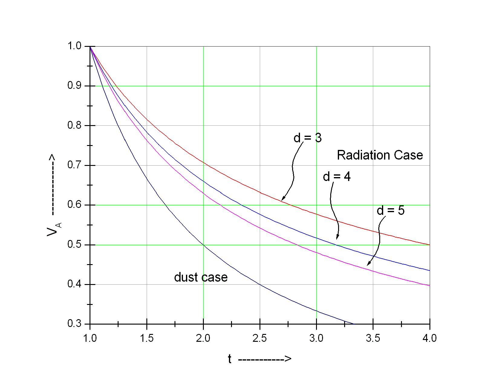
Figure 1: $v_{A}\sim t$ graph

It was pointed before that $\rho_{0}h\sim t^{-2}$ both in higher dimensions and 4D and also in radiation and dust case. For the prerecombination era in (d+1)- dimensional spacetime $B_{0}$ decreases with increasing dimensions, being maximum in 4D. Again for the postrecombination era (i.e, $\alpha=0$) the ambient magnetic field $B_{0}\sim t^{-2}$ for a fixed $`d$’. $B_{0}$ reaches asymptotically $t^{-2}$ for a very large number of dimensions in radiation case and the nature is same as the postrecombination era (see figure 2).

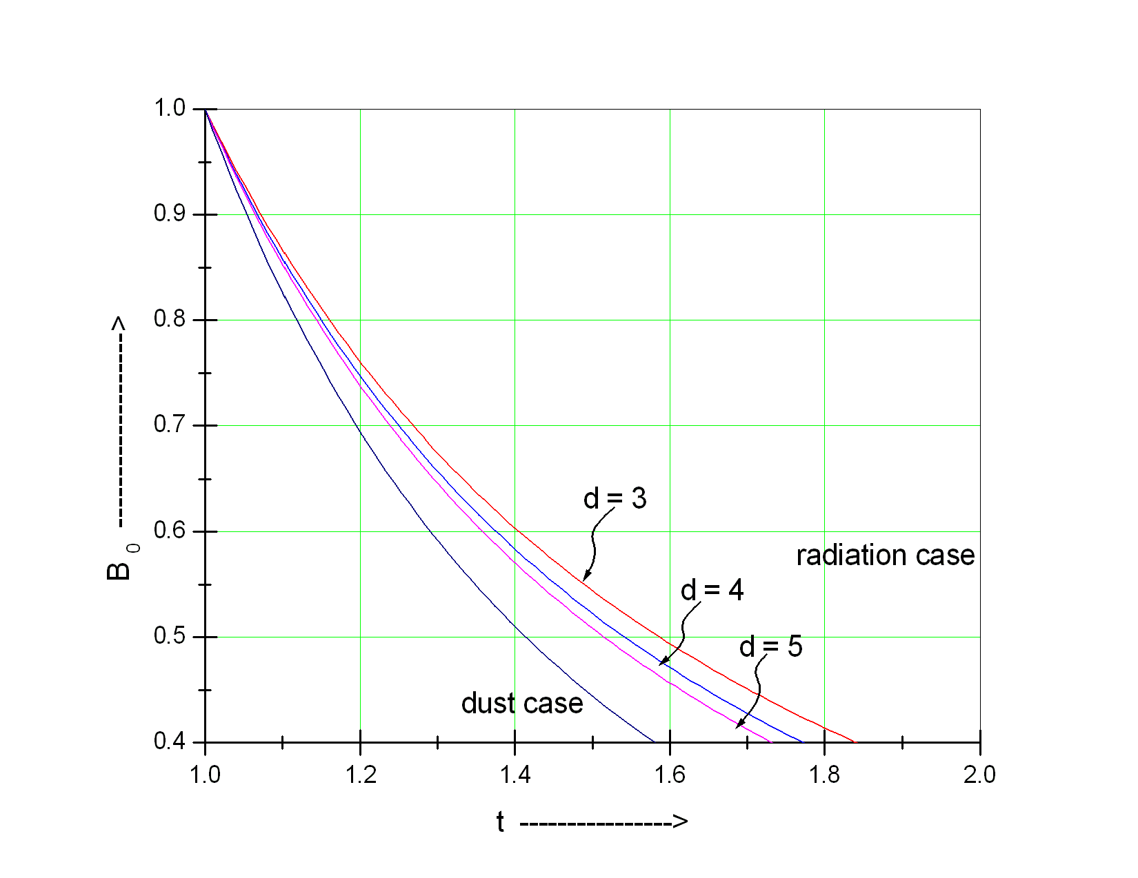
Figure 2: $B_{0}\sim t$ graph

The fact that $v_{A}$ decreases in an expanding background owes an explanation as follows : we know from classical idea that Alfvén wave is generated as in a transverse vibration in a string as an interplay between the unbalanced tension and inertia. When looked upon as lines of force the tension in the string comes out to be $\frac{B^{2}}{8\pi}$, the energy density of the magnetic field. Since with higher dimensions the volume increases the energy density, and consequently the magnetic field B also gets diluted. So the Alfvén velocity also decreases with increasing dimensions.

One can look at from a different standpoint also. As a consequence of flux conservation we may write

$$\dot{\Phi}=\frac{d}{dt}\int A^{d}Bds=\frac{d}{dt}\int t^{\frac{2}{1+\alpha}}=-\varepsilon~{}~{}~{}(e.m.f.)$$ (17)

Since the uniform ambient magnetic field does not produce an e.m.f we see that if $\varepsilon=0$, as the magnetic field must decay in time $t^{-\frac{2}{1+\alpha}}$ with respect to co-moving co-ordinates. This result is also same for 4D case as well as for higher dimensions. Thus as a consequence of magnetic flux conservation the field lines in an expanding universe are conformally diluted.

The theoretical result that with expansion the cosmic magnetic field decays much faster in HD compared to 4D may have non trivial implications in astrophysics. In a recent communication Gang Chen etal. [14] argued that if a primordial magnetic field did exist it should create vorticity and alfvén waves and finally cosmic microwave background (CMB) anisotropies. They later went to discuss the constrints that can be placed on the strength of such a field with the help of the CMB anisotropy data from WMAP experiment. The origin of the observed magnetic galactic field of a few $\mu G$ apparently coherent over a 10 kpc scale continues to evade satisfactory theoretical explanation. A plausible explanation may be the consequence of nonlinear amplification of a tiny seed field by galactic dynamo process [15]. CMB anisotropy data apparently suggests a seed field of $nG$  [14] strength. Now the dynamo mechanism being so efficient vis-a-vis amplification of the seed field at the early era it is quite likely to shoot up the seed field beyond the current value of a few $\mu G$. However that may introduce considerable anisotropy [16] in the manifestly homogeneous and isotropic FRW model. And here the HD model makes its presence felt in allowing the amplified field to decay much faster.

Now, putting $\gamma=\frac{d+1}{d}$ and $n=\frac{2}{d(1+\alpha)}$ in equation (15) we get finally,

$$t^{2}\frac{d^{2}v_{1}}{dt^{2}}+\frac{4d-4d\alpha-2}{d(1+\alpha)}t\frac{dv_{1}}{dt}+\frac{(2d-2d\alpha-2)(1-3\alpha)}{d(1+\alpha)^{2}}v_{1}~{}~{}~{}~{}~{}$$

$$+~{}t^{\frac{4\alpha}{1+\alpha}}v_{Ai}\times\nabla\times\nabla\times v_{1}\times v_{Ai}-t^{\frac{4\alpha}{1+\alpha}}C_{si}^{2}\nabla(\nabla.v_{1})=0$$ (18)

The above equation is quite complex. It can be simplified, however, if we consider the interesting case of the wave moving perpendicularly to both magnetic field and wave vector. In this case

$$v_{Ai}\times\nabla\times(\nabla\times v_{1}\times v_{Ai})=k_{i}^{2}v_{Ai}^{2}v_{1}$$ (19)

and

$$C_{si}^{2}\nabla(\nabla.v_{1})=-C_{si}^{2}k_{i}^{2}v_{1}$$ (20)

so the above equation gives

$$t^{2}\frac{d^{2}v_{1}}{dt^{2}}+\frac{4d-4d\alpha-2}{d(1+\alpha)}t\frac{dv_{1}}{dt}~{}~{}~{}~{}~{}~{}~{}~{}~{}~{}~{}~{}~{}~{}~{}~{}~{}~{}~{}~{}~{}~{}~{}~{}~{}~{}~{}~{}~{}~{}~{}~{}~{}~{}~{}~{}~{}~{}~{}~{}~{}~{}~{}~{}~{}~{}~{}~{}$$

$$+\left[\frac{(2d-2d\alpha-2)(1-3\alpha)}{d(1+\alpha)^{2}}+t^{\frac{4\alpha}{1+\alpha}}k_{i}^{2}(v_{Ai}^{2}+C_{si}^{2})\right]v_{1}=0$$ (21)

where the velocities,$C_{si}$ originates from the acoustic pressure and $v_{Ai}$ from the magnetic field. This is a Bessel type of equation of order, $p=\frac{d+d\alpha-2}{4d\alpha}$  $(\alpha\neq 0)$.

The equation (21) yields a general solution

$$v_{1}=t^{\frac{-3d+5d\alpha+2}{2d(1+\alpha)}}H_{(p)}\left[(v_{Ai}^{2}+C_{si}^{2})k_{i}\frac{1+\alpha}{2\alpha}t^{\frac{2\alpha}{1+\alpha}}\right]$$ (22)

Special Cases: We now briefly discuss the equation (22) for the special cases of ultra relativistic ($T>>m_{c}$) and also stiff fluid back ground. Evidently the prerelativistic case, $\alpha=0$ is not obtainable from the above equation and needs a separate treatment. So we take radiation and for the sake of completeness the stiff fluid case also.

I. Radiation Case : Putting $\alpha=\frac{1}{d}$ the equation (22) reduces to

$$v_{1}=t^{-\frac{(3d-7)}{2(d+1)}}H_{(p_{1})}\left[\frac{d+1}{2}(v_{Ai}^{2}+C_{si}^{2})k_{i}t^{\frac{2}{d+1}}\right]$$ (23)

where the order of the Henkel coefficient is given by $p_{1}=\frac{d-1}{4}$, the frequency of the oscillation $\sim t^{-\frac{d-1}{d+1}}$ and $(v_{Ai}^{2}+C_{s}^{2})^{\frac{1}{2}}$ is known as phase velocity. This mode corresponds to the magnetosonic or fast Alfvén mode because both velocities are simultaneously present. The result is identical to the flat space case also except that frequency redshifts here and is model dependent.

This wave is somewhat similar to an electromagnetic wave, since the time varying magnetic field is perpendicular to the direction of propagation but parallel to the magnetostatic field, whereas the time varying electric field is perpendicular to both the direction of propagation and the magnetostatic field which is a longitudinal wave. However, since the velocity of mass flow and also fluctuating mass density associated with the wave motion are both in the wave propagation direction this wave is called the magnetosonic longitudinal wave. The phase velocity $(v_{Ai}^{2}+C_{s}^{2})^{\frac{1}{2}}$ is independent of frequency so that it is a non dispersive wave. We see that the fluid velocity depends upon dimension also. It will reduce to Holcomb et al  [3] work for $d=3$. As noted earlier the attenuation of the wave propagation is more prominent in the higher dimensional regime compared to the 4D case$\left(v_{1}\sim t^{\frac{-3d+5}{2(d+1)}}\right)$. As the dimension ‘$d$’ increases indefinitely the damping finally becomes independent of ‘$d$’, $d\rightarrow\infty$ and $v_{1}\sim t^{-\frac{3}{2}}$ (see figure 3).

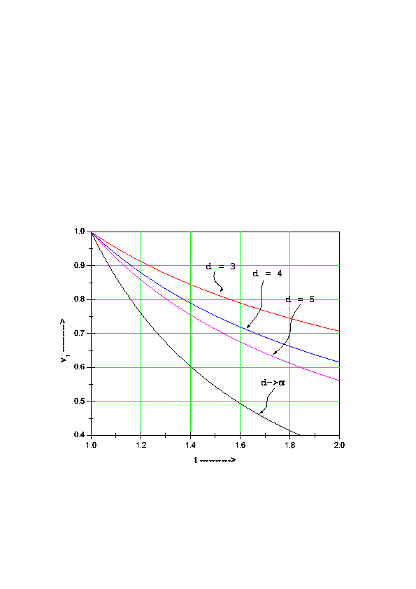
Figure 3: $v_{1}\sim t$ graph

Now if one can consider a relatively cold plasma such that the ‘pressure’ due to magnetic field far exceeds the acoustic pressure one may take $C_{si}=0$, this mode is known as pure or shear Alfvén wave. In this case only magnetic field is present, but the nature of wave will be same as magnetosonic wave. Another interesting feature comes out of the analysis. We have shown earlier  [1] like others in the related field that a free photon redshifts in the ultrarelativistic case and the field variables in the different plasma models also redshift identically. We get exactly similar result for the Alfvén mode also. Though not specifically emphasized in the earlier works this result, in our opinion, is not model independent. The fact that a conformally flat FRW mechanism is chosen in al our works all the field variables here scale with the conformal scale factor. A less symmetrical spacetime would possibly yield different results. We shall, however, subsequently see that the situation drastically changes in the non relativistic background.

On the other hand for very low magnetic field the acoustic pressure dominates and we get pure acoustic wave.

II. Stiff Fluid ($\alpha=1$): For the sake of completeness we also consider the stiff fluid case characterised by $\alpha=1$. Equation (22) gives ($C_{si}$= c = velocity of light ).

$$v_{1}=t^{\frac{d+1}{2d}}H_{\left(\frac{d-1}{2d}\right)}\left[(v_{Ai}^{2}+c^{2})k_{i}t\right]$$ (24)

However, the stiff fluid being not much physically relevant we skip discussion of this result.

III. Dust Case ($\alpha=0$): Here equation (21) becomes,

$$t^{2}\frac{d^{2}v_{1}}{dt^{2}}+\frac{4d-2}{d}t\frac{dv_{1}}{dt}+\left[\frac{2(d-1)}{d}+k_{i}^{2}v_{Ai}^{2}\right]v_{1}=0$$ (25)

It is clear that the form of the two equations corresponding to radiation and dust cases are distinctly different - one resembling the Bessel form while the other to an Euler type. In this case if the magnetic field is very strong so that the magnetic pressure is very much larger than the fluid pressure, then phase velocity of the magnetosonic wave becomes equal to the Alfvén wave velocity $v_{Ai}$. The second one has three solutions depending upon the discriminant $D=(d-2)^{2}-\left(2dk_{i}^{2}v_{Ai}^{2}\right)$:

(a) For $D>0$,

$$v_{1}=c_{1}t^{-\frac{1}{2d}[(3d-2)+\sqrt{D}]}+c_{2}t^{-\frac{1}{2d}[(3d-2)-\sqrt{D}]}$$ (26)

where $c_{1}$ and $c_{2}$ are constants. This is a general solution of equation (21). Here the above mode always dies out without much propagation.

(b) For $D=0$,

$$v_{1}=\left(c_{3}+c_{4}\ln t\right)t^{-\frac{(3d-2)}{2d}}$$ (27)

$c_{3}$ and $c_{4}$ are constants. It is apparent that $v_{1}$is least in the usual 3D. This result is somewhat intriguing when posited against the fact that the phenomena of damping is due to the background expansion, which is maximum in 3D. So other process may be in work besides the expansion rate in this case.

(c)  For $D<0$,

$$v_{1}=c_{5}t^{-\frac{3d-2}{2d}}\cos\left(\frac{\sqrt{D}}{2d}\ln t\right)+c_{6}t^{-\frac{3d-2}{2d}}\sin\left(\frac{\sqrt{D}}{2d}\ln t\right)$$ (28)

where $c_{5}$ and $c_{6}$ are constants. So we get damped oscillatory mode here, although the periodicity is not in cosmic time but in its logarithm. Hence the signature of of D which, in turn, depends on the dimension, external magnetic field and the density of the medium is crucial in determining whether a particular mode will be evanescent or propagating. In fact for oscillation to take place one should have $k_{i}v_{Ai}>\frac{d-1}{d}$. Now for dust $v_{Ai}$ is independent of $`d$’. So as number of dimension increase only very high frequency waves can propagate through a particular plasma medium. The extra dimensions, so to say, try to filter the frequency range. This finding is interesting but its astrophysical implications are yet to be looked into. The shear Alfvén waves are stationary in a certain frequency range which depends upon D. For higher frequencies, the waves do propagate; however, they are not oscillatory in the cosmic time, but in its logarithm.

3. Discussion

As physics in higher dimension is increasingly becoming an important and at the same time a distinct area of activity we are primarily interested in this work to investigate the effect of higher dimensions in the propagation of an electromagnetic wave in plasma media with an expanding background. As commented earlier in the introduction this work may be looked upon as continuation of our earlier work where acoustic and Alfvén modes are not considered. Here the background cosmology chosen is the simplest possible - FRW spacetime generalized to (d+1) dimensions. So the results we obtain differ essentially in some quantitative aspects without introducing much qualitative differences.

The interesting results may be briefly summarised as follows: We know that the expanding background generates a sort of damping such that the plasma variables like the amplitude of the wave, strength of the magnetic field etc. decay. Unlike mechanical damping the expansion creates a thinning of density of magnetic lines of force so that the velocity of the different modes keep on decreasing with time. Naturally for a contracting mode just the opposite will happen. We observe that this damping is the least in the usual 3D space compared to the HD space. As commented in the introduction this exercise may be looked upon as continuation of our earlier work where acoustic or Alfvén waves are not discussed. The locally measured frequencies resemble that of flat spacetime, though due to the expansion of the universe they do decay in time. We have found like others in the related field that in the ultra relativistic limit all modes redshift in the same scale as free photon. In the non relativistic limit, however, the situation drastically changes. Different modes redshift at different rates depending on the plasma density, magnitude of the external magnetic field and interestingly on number of dimensions. So here dimensions may embed a definite signature. These factors also dictate whether a particular mode becomes evanescent or can propagate through the medium. We find that as dimension increases only very high frequency waves can propagate but they are not oscillatory in cosmic time but in its logarithm. Finally coming back to the vexed question of a primordial magnetic field we find the field decays much faster in HD spacetime, which is a good news for the observed isotropy and homogeneity of the present universe because large magnetic field introduces anisotropy.

To end a final comment may be in order. We know that at the early phase when consideration of both higher dimensions and plasma phenomena are interesting the fluid was far from being perfect. Viscosity and heat processes were significant. Possible extension to this work could include formulating these equations for imperfect MHD including such effects as viscosity and finite conductivity. Nonlinear modes such as shocks could also be investigated. Judging by the complexity of the solutions it seems likely that more complicated modes may not be analytically solvable and may require extensive numerical analysis. Our simple analysis has kept intact the basic essence of MHD theory, highlighting the similarities and occasional differences with standard flatspace MHD, which complicated numerical analysis may mask.

Acknowledgment : One of us(SC) acknowledges the financial support of UGC, New Delhi for a MRP award.

References

- [1] D. Panigrahi and S. Chatterjee, JCAP 08 32 (2008).
- [2] D. Hooper and S. Profumo, ‘Dark Matter and Collider Phenomenology of Universal Extra Dimensions’, Physics Reports 453 p 27 - 115 (2007).
- [3] K. A. Holcomb and T. Tajima, Phy. Rev. D40 3809(1989);
- [4] K. A.Holcomb, Astrophysical. J. 362 381(1990).
- [5] C. P. Dettmann, N. E. Frankel,Phys. Rev. D48 5655 (1993)
- [6] A. Sil, N. Banerjee and S. Chatterjee Phy. Rev. D53 7365 (1996) ;
- [7] A. Banerjee, S. Chatterjee, A. Sil and N. Banerjee, Phy. Rev. D50 1161 (1994).
- [8] D. A. Macdonald and K. Thorne, Mon. Not. R. Astron. Soc. 198 345 (1982).
- [9] R. Arnowitt, S. Deser and C. W. Misner, in Gravitation: An Introduction to current Research, edited by L. witten ( Wiley), New York, (1962).
- [10] Pisin Chen and Kwang- Chang Lai, Phys. Rev. Lett. 99 231302 (2007).
- [11] M. Giovannini, Int.J.Mod.Phys. D13 391 (2004)
- [12] S. Chatterjee and B. Bhui, Mon. Not. R. Astron. Soc. 108, 252 (1990).
- [13] S. Wienberg, Gravitation and Cosmology (Wiley, new york, 1972) P-51
- [14] Gang Chen, Pia Mukherjee, Tina Kahniashili, Bharat Ratra, Yun Wang, Astrophysical. J. 611 665 (2004)
- [15] E. G. Zweibel, Astrophysical. J. 329L1(1998)
- [16] B. Ya. Zel’dovich, A. A. Ruzaikin and D. D. Sokoloff, Magnetic Fields in Astrophysics (New York: Gordon and Breach) (1983)