A quantum volume hologram

Abstract

We propose a new scheme for parallel spatially multimode quantum memory for light. The scheme is based on counter-propagating quantum signal wave and strong classical reference wave, like in a classical volume hologram, and therefore can be called a quantum volume hologram. The medium for the hologram consists of a spatially extended ensemble of atoms placed in a magnetic field. The write-in and read-out of this quantum hologram is as simple as that of its classical counterpart and consists of a single pass illumination. In addition we show that the present scheme for a quantum hologram is less sensitive to diffraction and therefore is capable of achieving higher density of storage of spatial modes as compared to previous proposals. A quantum hologram capable of storing entangled images can become an important ingredient in quantum information processing and quantum imaging.

I introduction

Quantum memory for light is an essential part of quantum information protocols, such as quantum repeaters, distributed quantum computation, and quantum networks. A number of approaches based on storage in atomic ensembles were developed recently, including quantum non-demolition (QND) interaction, electromagnetically induced transparency (EIT), Raman interaction and photon echo. For a comprehensive recent review on quantum interfaces between light and matter see Hammerer08 . Multimode quantum memories are in the center of current research due to their potential for enhanced storage capacity and state purification and error correction,e.g., in quantum repeaters Simon07 .

Spatially–multimode parallel quantum protocols for light without memory have been central for the field of quantum imaging. Examples are quantum holographic teleportation Sokolov01 ; Gatti04 and telecloning Magdenko07 , and quantum dense coding of optical images Golubev06 . The spatially multimode light in an entangled Einstein - Podolsky - Rosen (EPR) quantum state Kolobov99 has been recently experimentally demonstrated via four-wave mixing in Lett08 .

A quantum memory protocol based on a QND interaction, for the single–mode case experimentally demonstrated in Julsgaard04 , achieves storage in the ground state of an ensemble of spin–polarized atoms. An extension of the QND–based scheme of quantum memory to spatially multimode configuration, able to store quantum images, has been proposed recently in Vasilyev08 . In this proposal two passes of light are required to store, and another two – to retrieve quantum state of an image from the hologram. In addition, perfect squeezing of the initial state of light and/or atoms is required for an ideal performance of the holographic memory.

Another approach to the multimode quantum memory based on phase-matched backward propagation retrieval out of the EIT and the Raman type memories has been recently proposed for the multiple frequency-encoded qubits storage in a single ensemble Shurmacz08 . A gradient echo memory has been proposed for storage of several frequency encoded modes Sellars08 .

The optical image storage has been demonstrated in recent experiments Camacho07 ; Shuker08 ; Vudyasetu08 . There was observed Camacho07 a several nanoseconds delay of optical pulses which contain on average less than one photon and carry two-dimensional images. The delay has been achieved by using slow light in an atomic ensemble. However, preservation of quantum field properties was not demonstrated in the paper. The storage of classical images in a warm atomic vapor by EIT interaction has been investigated in Shuker08 ; Vudyasetu08 .

In this paper we present a new scheme of the multimode quantum memory which we call a quantum volume hologram. Our proposal makes use of two concepts. The first one stems from a volume hologram, proposed by Denisyuk Denisyuk62 for classical storage of optical images. The volume hologram is written by the counter-propagating signal and reference waves. There are two sublattices, produced by the waves interfering in the medium, each of them stores one quadrature of the signal field. Since both quadratures are stored, there are no virtual and real images during the readout, by contrast to a thin hologram.

The second concept comes from Muschik06 where it was shown that a combination of a constant magnetic field with the QND interaction allows to couple two components of the collective atomic spin used for the quantum memory to two quadratures of light.

In the present paper we propose to write volume hologram (which implies the counter-propagating geometry) onto an atomic ensemble with spins rotating in a constant magnetic field. Hence, in our model all degrees of freedom of atoms and light are symmetrically involved in the interaction. We show that an input state of spatially–multimode light can be written onto the quantum volume hologram in a single pass. A sideband (with respect to the carrier frequency of the strong field $\omega$) $+\Omega$ spectral component of light is written onto the collective spin coherence wave, which propagates in the medium with a certain phase velocity.

Our analysis shows, that the volume hologram for the ground state spin $J=1/2$, when considered in the limit of a single spatial mode, has features similar to those described in Nunn07 for $\Lambda$–scheme of atomic levels (possible only for $J>1/2$). It appears that an effective increase in the number of the system degrees of freedom due to the counter-propagating geometry in combination with the spin rotation has an effect similar to the increased complexity of the atomic level structure in the $\Lambda$–scheme based memories.

The paper is organized as follows. First, we discuss the basics of the model and derive the light and matter equations of motion in the paraxial approximation using averaging over fast oscillations in space and time. Next, we consider transfer of an input multimode quantum state encoded in the signal wavefront at the write and readout stages. Finally, the stored transverse modes number is estimated for the volume and the thin Vasilyev08 quantum hologram and we come to conclusion.

II Single pass volume hologram with spatial resolution

The scheme, illustrating our quantum memory protocol is shown in Fig. 1.

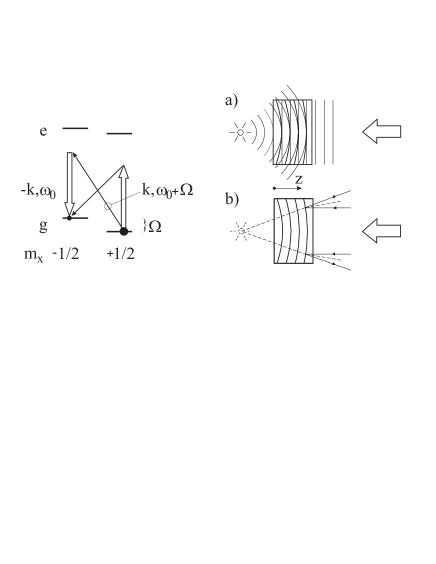
Figure 1: Schematic of the level structure and of the write (a) and readout (b) stages of quantum volume hologram

We consider an ensemble of motionless atoms which we for simplicity assume to have an angular momentum of $J=1/2$ both in the ground and in the excited states, located at random positions. The long-lived ground state spin of an atom ${\vec{J}}^{a}$ is initially oriented along the constant magnetic field in the vertical direction $x$. The atomic spins rotate around the vertical axis with a circular frequency $\Omega$. A classical off-resonant $x$-polarized plane wave at frequency $\omega_{0}$ with a slowly varying amplitude $A_{x}$ (assumed to be real) propagates in $-z$ direction. The input signal wave is a weak quantized $y$-polarized field at the same frequency $\omega_{0}$, propagating in $+z$ direction. In what follows we consider this multimode input field with a slowly varying amplitude $A_{y}(\vec{r},t)\ll A_{x}$ in the paraxial approximation.

In order to construct the Hamiltonian of the system we first consider an atomic layer with the thickness (in $z$ direction) smaller than $\lambda$. Within this layer the phase difference between the signal field and the driving wave is constant. Hence, the interaction within the slice is described by the well known quantum non-demolition (QND) Hamiltonian Hammerer08 . The QND light-matter interaction in the each layer leads to two basic effects: (i) the Faraday rotation of light polarization due to longitudinal quantum $z$-component of collective atomic spin of the slice; and (ii) the atomic spin rotation, caused by the unequal light shifts of the ground state sub-levels with $m_{z}=\pm 1/2$ in the presence of quantum fluctuations of circular light polarizations. The relevant part of the Hamiltonian is Hammerer08 :

$$H=\frac{2\pi k_{0}|d|^{2}}{\omega_{eg}-\omega_{0}}\int_{V}d\vec{r}\sum_{a}J_{z}^{a}(t)S_{z}(\vec{r},t)\delta(\vec{r}-\vec{r}_{a}).$$ (1)

Here $\omega_{eg}$ is the frequency of the atomic transition, $d$ is the dipole matrix element, and $k_{0}=\omega_{0}c$. For the counterpropagating signal and driving waves, the $z$-component of the Stokes vector $S_{z}(\vec{r},t)=2A_{x}\,Im\left[A_{y}(\vec{r},t)e^{2k_{0}z}\right]$ in (1) rapidly (i.e. on the scale $\lambda$) oscillates along $z$. The amplitude $A_{y}$ is defined via

$$A_{y}(z,\vec{\rho},t)=\int\frac{dk_{z}}{2\pi}\int\frac{d\vec{q}}{(2\pi)^{2}}\sqrt{\omega(k)/k_{0}}\,a_{y}(\vec{k})\exp[i(\vec{q}\cdot\vec{\rho}+(k_{z}-k_{0})z-(\omega(k)-\omega_{0})t)],$$

here $a_{y}(\vec{k})$ and $a_{y}^{\dagger}(\vec{k})$ are the annihilation and creation operators for the wave $\vec{k}$, which obey standard commutation relations $[a_{y}(\vec{k}),a_{y}^{\dagger}(\vec{k}\,^{\prime})]=(2\pi)^{3}\delta(\vec{k}-\vec{k}\,^{\prime})$, $[a_{y}(\vec{k}),a_{y}(\vec{k}\,^{\prime})]=0$. By using these commutation relations in the paraxial approximation, one finds Kolobov99 the commutation relation for the slowly varying amplitude of the quantized signal field $A_{y}$,

$$[A_{y}(z,\vec{\rho},t),A_{y}^{\dagger}(z^{\prime},\vec{\rho}\,^{\prime},t)]\equiv c\tilde{\delta}(\vec{r}-\vec{r}\,^{\prime})\approx$$ (2)

$$c\left(1-\frac{i}{k_{0}}\frac{\partial}{\partial z}-\frac{1}{2k^{2}_{0}}\nabla^{\,2}_{\bot}\right)\delta(\vec{r}-\vec{r}\,^{\prime}),$$

where $\vec{r}=(\vec{\rho},z)$, $\vec{k}=(\vec{q},k_{z})$. We do not consider here the $y$-polarized quantized field co-propagating with the driving wave because its evolution is independent of the signal wave under consideration.

We introduce the density of the collective spin as $\vec{J}(\vec{r})=\sum_{a}\vec{J}^{a}\delta(\vec{r}-\vec{r}_{a})$. The averaged over random positions of the atoms commutation relation for the $y$, $z$ components of the collective spin is

$$\overline{[J_{y}(\vec{r}),J_{z}(\vec{r}\,^{\prime})]}=i\sum_{a}\langle J_{x}^{a}\rangle\overline{\delta(\vec{r}-\vec{r}_{a})\delta(\vec{r}\,^{\prime}-\vec{r}_{a})}^{a}=in_{a}\langle J_{x}^{a}\rangle\delta(\vec{r}-\vec{r}\,^{\prime}).$$

Here $n_{a}$ is the average density of atoms. The field-like variable for the spin subsystem,

$$B(\vec{r},t)=\{J_{y}(\vec{r},t)+iJ_{z}(\vec{r},t)\}/\sqrt{2n_{a}\langle J_{x}^{a}\rangle},$$

obeys the standard boson commutation relation:

$$\overline{[B(\vec{r},t),B^{{\dagger}}(\vec{r}\,^{\prime},t)]}=\delta(\vec{r}-\vec{r}\,^{\prime}).$$ (3)

In view of the fact that the atoms are prepared in the spin up state, the operator $B^{{\dagger}}$ can be considered as the creation operator for atoms in the spin down state, or the collective projection operator $|+1/2\rangle\to|-1/2\rangle$.

The full Hamiltonian of our model includes the energy of a free electromagnetic field, the interaction of the atomic spin with constant magnetic field and the effective Hamiltonian of the QND interaction. The Hamiltonian reads,

$$H=\int_{V}d\vec{r}\left\{\frac{\hbar\omega_{0}}{c}A_{y}^{\dagger}(z,\vec{\rho},t)\,A_{y}(z,\vec{\rho},t)+\hbar\Omega\,B^{\dagger}(z,\vec{\rho},t)\,B(z,\vec{\rho},t)-\right.$$ (4)

$$\left.\frac{\sqrt{2}\pi k_{0}|d|^{2}}{\omega_{eg}-\omega_{0}}\sqrt{n\langle J_{x}^{a}\rangle}A_{x}(z,t)\big{[}B(z,\vec{\rho},t)-h.c.\big{]}\big{[}A_{y}(z,\vec{\rho},t)e^{i2k_{0}z}-h.c.\big{]}\right\}.$$

We describe the evolution of our system in the Heisenberg picture. Using the commutation relations (2) and (3) for the field and atomic variables, after simple transformations we obtain:

$$\left(\frac{\partial}{\partial z}-\frac{i}{2k_{0}}\nabla^{\,2}_{\bot}+\frac{1}{c}\frac{\partial}{\partial t}\right)A_{y}(z,\vec{\rho},t)=\frac{\kappa}{\sqrt{LT}}\,{\rm Im}B(z,\vec{\rho},t)e^{-i2k_{0}z},$$ (5)

$$\frac{\partial}{\partial t}B(z,\vec{\rho},t)=-i\Omega B(z,\vec{\rho},t)+\frac{\kappa}{\sqrt{LT}}{\rm Im}\left[A_{y}(z,\vec{\rho},t)e^{i2k_{0}z}\right].$$ (6)

Here $T$ is the duration of the flat-top pulse of the driving field and $L$ is the atomic cell length. The dimensionless coupling constant

$$\kappa=\frac{2\pi k_{0}|d|^{2}}{\hbar(\omega_{eg}-\omega_{0})}\sqrt{2n_{a}\langle J_{x}^{a}\rangle A_{x}^{2}LT},$$ (7)

should be of the order unity for the memory to work. The coupling constant can be written as $\kappa^{2}=\alpha_{0}\eta$, where $\alpha_{0}$ is the resonant optical depth and $\eta$ is the probability of spontaneous emission Hammerer08 . Since $\eta\ll 1$ is required in order to neglect the effect of spontaneous emission from the excited atomic level, the usual condition for an efficient quantum interface $\alpha_{0}=\lambda^{2}n_{a}L/2\pi\gg 1$ should be fulfilled. We introduce the Fourier transform via

$$a(z,\vec{q},t)=\int d\vec{\rho}\,A_{y}(z,\vec{\rho},t)e^{-i\vec{q}\,\vec{\rho}},$$ (8)

and similar for atomic variables, and arrive at the set of basic equations in the Fourier domain,

$$\left(\frac{\partial}{\partial z}+i\frac{\vec{q}\,^{2}}{2k_{0}}+\frac{1}{c}\frac{\partial}{\partial t}\right)a(z,\vec{q},t)=\frac{\kappa}{\sqrt{LT}}\frac{1}{2i}\left[b(z,\vec{q},t)-b^{\dagger}(z,-\vec{q},t)\right]e^{-i2k_{0}z},$$ (9)

$$\frac{\partial}{\partial t}b(z,\vec{q},t)=-i\Omega b(z,\vec{q},t)+\frac{\kappa}{\sqrt{LT}}\frac{1}{2i}\left[a(z,\vec{q},t)e^{i2k_{0}z}-a^{\dagger}(z,-\vec{q},t)e^{-i2k_{0}z}\right].$$ (10)

The considered above field and atomic amplitudes are rapidly oscillating at frequency of the order $\Omega$. In what follows we introduce the slowly varying amplitudes of collective spin $b_{\pm k}(z,\vec{q},t)$ in the rotating at $\Omega$ frame, and slowly varying amplitudes $a_{\pm\Omega}(z,\vec{q},t)$ for the signal field sidebands at frequencies $\omega_{0}\pm\Omega$.

Next, we should take into account that the field amplitudes are defined as slowly varying along the $z$ axis, but the spin amplitudes are not, as seen from (10). The fast modulation of the collective spin at the longitudinal spatial frequency $2k_{0}$ is just a consequence of the counter propagating geometry of the volume hologram. The thin atomic slices discussed above have a length of the order of a fraction of $\lambda$. This imposes limitations on the atomic motion during the storage time: the atoms should not transport coherence to another slice. A solid state, an optical lattice, or an ultra cold atomic ensemble should be used to fulfil this condition. The slow in space and time variables look like

$$a_{\pm\Omega}(z,\vec{q},t)=a(z,\vec{q},t)e^{\pm i\Omega t},$$ (11)

$$b_{\pm k}(z,\vec{q},t)=b(z,\vec{q},t)e^{i(\Omega t\mp 2k_{0}z)}.$$

Quantum memory is realized via the dynamical coupling between $a_{\Omega}(z,\vec{q},t)$ and $b_{k}(z,\vec{q},t)$. We insert these variables into (9), (10) and perform averaging on a time scale $1/\Omega\ll t_{av}\ll T$ and on a spatial scale in $z$ direction $\lambda\ll z_{av}\ll L$. This implies that the pulse duration and the cell length are taken large enough, $\Omega T\gg 1$ and $k_{0}L\gg 1$, where the last condition is typical also for classical volume holograms.

The equations of motion read,

$$\frac{\partial}{\partial z}a_{\Omega}(z,\vec{q},t)=\left[-\frac{1}{c}\frac{\partial}{\partial t}+i\left(\frac{\Omega}{c}-\frac{\vec{q}\,^{2}}{2k_{0}}\right)\right]a_{\Omega}(z,\vec{q},t)-i\frac{\kappa}{2\sqrt{LT}}b_{k}(z,\vec{q},t),$$ (12)

$$\frac{\partial}{\partial t}b_{k}(z,\vec{q},t)=-i\frac{\kappa}{2\sqrt{LT}}a_{\Omega}(z,\vec{q},t).$$ (13)

In what follows we neglect the retardation effects. Both the pulse length in space, estimated as $c/\delta\Omega$, where $\delta\Omega$ is the signal spectral width, and the spatial length $c/\Omega$ of modulation at frequency $\Omega$ are assumed to be much larger than the cell length, hence $\delta\Omega/c\ll\Omega/c\ll 1/L$. This allows to omit the terms $\sim 1/c$ on the right side of (12) as compared to the term $\sim b/\sqrt{LT}$, which is estimated as $\sim a/L$. Here we make use of (13) and find for typical values $\kappa\sim 1$ and $t\sim T$ an estimate $b\sim\sqrt{T/L}\,a$.

Next, we go over to the amplitudes

$$\tilde{a}_{\Omega}(z,\vec{q},t)=a_{\Omega}(z,\vec{q},t)\exp\left(i\frac{q^{2}}{2k_{0}}z\right),\qquad\tilde{b}_{k}(z,\vec{q},t)=b_{k}(z,\vec{q},t)\exp\left(i\frac{q^{2}}{2k_{0}}z\right),$$ (14)

and arrive at the equations

$$\frac{\partial}{\partial z}\tilde{a}_{\Omega}(z,\vec{q},t)=-i\frac{\kappa}{2\sqrt{LT}}\,\tilde{b}_{k}(z,\vec{q},t),\qquad\frac{\partial}{\partial t}\tilde{b}_{k}(z,\vec{q},t)=-i\frac{\kappa}{2\sqrt{LT}}\,\tilde{a}_{\Omega}(z,\vec{q},t).$$ (15)

As compared to the equations, previously discussed (e.g., Mishina06 ; Nunn07 and references therein) for the $\Lambda$–scheme Raman–type models of spatially single mode quantum memory, we do not encounter in (15) the deleterious effect of the Stark shift of atomic levels by a classical control pulse. The level shift makes the phase matching and evolution more complicated, especially for a time–dependent profile of the control field. This simplification is due to the more symmetrical nature of the QND interaction.

It follows from (15) that in our parallel quantum memory, based on the volume hologram, the signal and the spin coherence waves with an arbitrary $\vec{q}$ (in paraxial approximation) are interacting like the waves propagating along $z$ direction in a spatially single mode Raman–type memory. The diffraction does not modify the state exchange between light and matter, and our memory is able to store as many orthogonal spatial mode with different $\vec{q}$ as one can fit into a hologram of transverse area $S$. We take $\Delta q_{x,y}\sim 2\pi/\sqrt{S}$, $|\vec{q}|\ll 2\pi/\lambda$, and assume that the number of transverse modes is much less than $4S/\lambda^{2}$.

The solution in terms of the amplitudes (14) is found as an extension to the spatially multimode case of the results previously obtained for the Raman–type model,

$$\tilde{a}_{\Omega}(z,\vec{q},t)=\tilde{a}_{\Omega}(0,\vec{q},t)-\frac{\kappa}{2\sqrt{LT}}\int_{0}^{t}dt^{\prime}\sqrt{\frac{z}{t-t^{\prime}}}\,J_{1}\left(\kappa\sqrt{\frac{z(t-t^{\prime})}{LT}}\right)\tilde{a}_{\Omega}(0,\vec{q},t^{\prime})$$ (16)

$$-i\frac{\kappa}{2\sqrt{LT}}\int_{0}^{z}dz^{\prime}\,J_{0}\left(\kappa\sqrt{\frac{(z-z^{\prime})t}{LT}}\right)\tilde{b}_{k}(z^{\prime},\vec{q},0),$$

$$\tilde{b}_{k}(z,\vec{q},t)=\tilde{b}_{k}(z,\vec{q},0)-\frac{\kappa}{2\sqrt{LT}}\int_{0}^{z}dz^{\prime}\sqrt{\frac{t}{z-z^{\prime}}}\,J_{1}\left(\kappa\sqrt{\frac{(z-z^{\prime})t}{LT}}\right)\tilde{b}_{k}(z^{\prime},\vec{q},0)$$ (17)

$$-i\frac{\kappa}{2\sqrt{LT}}\int_{0}^{t}dt^{\prime}\,J_{0}\left(\kappa\sqrt{\frac{z(t-t^{\prime})}{LT}}\right)\tilde{a}_{\Omega}(0,\vec{q},t^{\prime}).$$

Consider the dimensionless coordinates and amplitudes,

$$\frac{z}{L}=\xi,\quad\frac{t}{T}=\tau,\quad a_{\Omega}(z,\vec{q},t)\sqrt{T}=\alpha_{\Omega}(\xi,\vec{q},\tau),\quad b_{k}(z,\vec{q},t)\sqrt{L}=\beta_{k}(\xi,\vec{q},\tau).$$ (18)

Here $\alpha(z,\vec{\rho},t)^{\dagger}\alpha(z,\vec{\rho},t)$ corresponds to the number of signal photons per $cm^{2}$ of the beam cross section during the interaction time $T$, and $\beta(z,\vec{\rho},t)^{\dagger}\beta(z,\vec{\rho},t)$ gives the number of flipped spins per $cm^{2}$ of the hologram cross section at the length $L$. The equations above become

$$\tilde{\alpha}_{\Omega}^{(out)}(\vec{q},\tau)=\int_{0}^{1}d\tau^{\prime}G_{1}(\tau-\tau^{\prime},1)\tilde{\alpha}_{\Omega}^{(in)}(\vec{q},\tau^{\prime})-i\int_{0}^{1}d\xi^{\prime}G_{0}(1-\xi^{\prime},\tau)\tilde{\beta}_{k}^{(in)}(\xi^{\prime},\vec{q}),$$ (19)

$$\tilde{\beta}_{k}^{(out)}(\xi,\vec{q})=\int_{0}^{1}d\xi^{\prime}G_{1}(\xi-\xi^{\prime},1)\tilde{\beta}_{k}^{(in)}(\xi^{\prime},\vec{q})-i\int_{0}^{1}d\tau^{\prime}G_{0}(1-\tau^{\prime},\xi)\tilde{\alpha}_{\Omega}^{(in)}(\vec{q},\tau^{\prime}),$$ (20)

where $\tilde{\alpha}_{\Omega}^{(in)}(\vec{q},\tau)=\tilde{\alpha}_{\Omega}(0,\vec{q},\tau)$, $\tilde{\alpha}_{\Omega}^{(out)}(\vec{q},\tau)=\tilde{\alpha}_{\Omega}(1,\vec{q},\tau)$, and $\tilde{\beta}^{(in)}(\xi,\vec{q})=\tilde{\beta}_{k}(\xi,\vec{q},0)$, $\tilde{\beta}^{(out)}(\xi,\vec{q})=\tilde{\beta}_{k}(\xi,\vec{q},1)$. The integral kernels are given by

$$G_{0}(p,q)=\frac{\kappa}{2}J_{0}(\kappa\sqrt{pq}),\quad G_{1}(p,q)=\delta(p)-\frac{\kappa}{2}J_{1}(\kappa\sqrt{qp})\sqrt{q/p}\,\theta(p),$$ (21)

with the $n$th Bessel function of the first kind denoted by $J_{n}$.

Similar to the analysis of Nunn07 , we make use of the fact that the kernels $G_{0,1}$ share eigen functions,

$$G_{0}(1-x,y) = \sum_{i}\phi_{i}(y)\lambda_{i}\phi_{i}(1-x),$$ (22)

$$G_{1}(y-x,1) = \sum_{i}\phi_{i}(y)\mu_{i}\phi_{i}(1-x),$$

and their eigen values satisfy the constraint $\lambda_{i}^{2}+\mu_{i}^{2}=1$ for all $i$. By applying the variables decomposition of the form

$$\tilde{\alpha}^{(in)}_{\Omega}(\vec{q},\tau) = \sum_{j}\tilde{\alpha}^{(in)}_{\Omega,j}(\vec{q})\phi_{j}(1-\tau),$$ (23)

$$\tilde{\beta}^{(in)}_{k}(\xi,\vec{q}) = \sum_{j}\tilde{\beta}^{(in)}_{k,j}(\vec{q})\phi_{j}(1-\xi),$$

one arrives at the input–output transformation for one cycle of the light–matter interaction:

$$\tilde{\alpha}^{(out)}_{\Omega}(\vec{q},\tau) = \sum_{i}\left[\mu_{i}\tilde{\alpha}^{(in)}_{\Omega,i}(\vec{q})-i\lambda_{i}\tilde{\beta}^{(in)}_{k,i}(q)\right]\phi_{i}(\tau),$$ (24)

$$\tilde{\beta}^{(out)}_{k}(\xi,\vec{q}) = \sum_{i}\left[-i\lambda_{i}\tilde{\alpha}^{(in)}_{\Omega,i}(\vec{q})+\mu_{i}\tilde{\beta}^{(in)}_{k,i}(q)\right]\phi_{i}(\xi).$$

The transformation is of a beamsplitter type, it is unitary and hence respects the correct bosonic commutation relations. The Eq. (24) shows, that if the light signal stored in an atomic hologram has the temporal profile of an eigen mode of $G_{0}$ with the eigen value $\lambda_{i}$ close to unity, the initial state of the atomic spins in the mode $i$ in erased since the corresponding eigen value $\mu_{i}$ is close to zero.

In order to read out the image stored in the hologram, one has to repeat the procedure and pass another classical light pulse through the atoms. To describe the whole write–readout cycle of parallel quantum memory, we combine the transformations $\left\{{\tilde{\alpha}_{\Omega}}^{W(in)}(\vec{q},\tau),\,{\tilde{\beta}_{k}}^{W(in)}(\xi,\vec{q})\right\}\to{\tilde{\beta}_{k}}^{W(out)}(\xi,\vec{q})$ for the write stage, and $\left\{{\tilde{\alpha}_{\Omega}}^{R(in)}(\vec{q},\tau),\,{\tilde{\beta}_{k}}^{R(in)}(\xi,\vec{q})={\tilde{\beta}_{k}}^{W(out)}(\xi,\vec{q})\right\}\to{\tilde{\alpha}_{\Omega}}^{R(out)}(\vec{q},\tau)$ for the readout stage, and restore the diffraction factor (see (14)). This yields,

$$\alpha_{\Omega}^{R(out)}(\vec{q},\tau)=\exp\left(-i\frac{q^{2}}{2k_{0}}L\right)\sum_{i}\left\{\mu_{i}\alpha_{\Omega,i}^{R(in)}(\vec{q})-i\lambda_{i}\sum_{j}f_{ij}\left[\mu_{j}\tilde{\beta}_{k,j}^{W(in)}(\vec{q})-i\lambda_{j}\alpha_{\Omega,j}^{W(in)}(\vec{q})\right]\right\}\phi_{i}(\tau),$$ (25)

where

$$f_{ij}=\int_{0}^{1}d\xi\phi_{i}(1-\xi)\phi_{j}(\xi),$$ (26)

is the eigen functions overlap factor. In Fig.2 we plot the first eigen functions evaluated numerically.

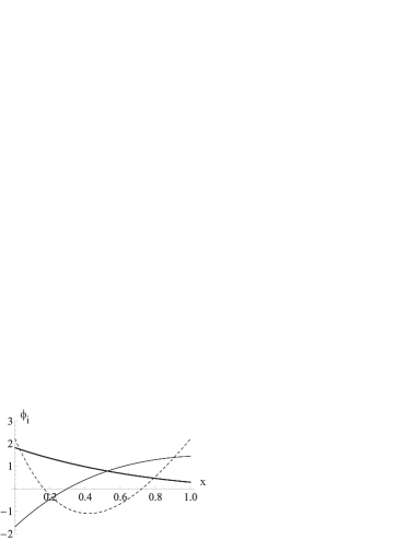
Figure 2: The first three eigen functions: $\phi_{1}$, $\phi_{2}$, and $\phi_{3}$ (the bold, thin and dashed line respectively) for $\kappa=4$. The eigen values are $\lambda_{1}\approx 0.988$, $\lambda_{2}\approx-0.518$, and $\lambda_{3}\approx 0.043$.

The Eq.(25) shows that the input (at the write stage) quantized amplitude of the signal field in the $i$th eigen mode gets restored at $z=L$ with the factor $\sim\exp\left(-iq^{2}L/2k_{0}\right)\lambda_{i}^{2}f_{ii}$. Like in the Raman–type schemes, our model demonstrates the time reversal symmetry between the input and output modes, as follows from the input (II) and output (25) signal decomposition. The read-in coupling parameter $\kappa\approx 4$ and a read-out coupling parameter in excess of 20 is required to achieve memory efficiency $\geq 0.95$ Nunn07 .

The storage capacity, that is the number of transverse modes that the quantum hologram can store is one of the most important parameters for the memory applications. The memory capacity of the previously proposed Vasilyev08 thin quantum hologram is strongly limited by diffraction. Namely, the diffraction spread of an input image element of the linear size $d$ should be small, $\lambda/d\cdot L\leq d$. Hence, the number $N$ of the resolved by the thin hologram image elements (modes) is determined by the sample Fresnel number $F_{N}$, so that $N\sim S/d^{2}\sim S/\lambda L=F_{N}$, where $S$ is the sample cross section. The authors of Shurmacz08 who have considered the multiple optical modes storage in an atomic ensemble with appropriately phase-matched backward propagating retrieval also estimate the number of stored transverse modes to be equal to $F_{N}$.

In comparison, the effect of diffraction on the signal wavefront stored in the volume hologram is the same as in free space and can be compensated simply by using a lens system with the input focal plane at $z=0$. The limitation on the capacity for the volume hologram comes first from the paraxial approximation $\lambda/d\leq\varepsilon$, where $\varepsilon\ll 1$ is the small parameter of the paraxial approximation. The second limitation is due to the geometry of the sample, $\lambda/d\cdot L\approx\sqrt{S}$, so that the quantized waves propagate inside the atomic cell. Hence the number of stored modes in the volume hologram is estimated to be $S/d^{2}\sim{\rm min}\{\varepsilon^{2}S/\lambda^{2},\,F_{N}^{2}\}$. For not too elongated samples with $\sqrt{S}/L\geq\varepsilon$ the number of modes is equal to $\varepsilon^{2}S/\lambda^{2}$ which is larger than for memories proposed so far. There are indications that for the co-propagating write-in and read-out $\Lambda$– scheme based multimode memories the capacity is also of the order of $\varepsilon^{2}S/\lambda^{2}$ Sorensen09 .

III Conclusions

We have presented an extension of the classical volume hologram into the quantum domain. The volume quantum hologram can store entangled and other quantum images and offers a new approach to a parallel spatially multimode quantum memory for light. The equations of motion for the quantized field and spin coherence waves are derived and examined in paraxial approximation. Our analysis could be of use for the spatially–multimode generalization of other quantum memory models.

The counter–propagating geometry of the classical and quantized fields, combined with the spins rotation in a constant magnetic field, allows for the efficient quantum image transfer between light and matter in a single pass of light. The volume hologram proposed here does not require any extra operations, such as squeezing, in order to achieve, in principle, perfect performance.

In our scheme, different spatial modes of the incoming field are stored in the corresponding orthogonal spatial modes of the atomic ensemble. We show that the quantum volume hologram is less sensitive to diffraction and is capable of storing more spatial modes as compared to the previously proposed Vasilyev08 thin hologram in the co–propagating geometry.

Although we considered spin $1/2$ atoms, our analysis can be easily generalized to an arbitrary angular momentum states in alkali atoms provided that the optical detuning is greater than the excited state hyperfine structure Hammerer08 . Future work on volume quantum holograms will include modified geometries of the interacting waves which should allow for relaxing of the requirement of motionless atoms, as well as studies of multimode quantum entanglement between light and matter.

We would like to thank Anders Sørensen for fruitful discussions. This research has been funded by the European Commission FP7 under the grant agreement n 221906, project HIDEAS. The authors also acknowledge the support of the Russian Foundation for Basic Research under the projects 05-02-19646, 08-02-00771, and 08-02-92504 (D.V.), and the support by INTAS (Grant 7904). Part of the research was performed within the framework of GDRE ”Lasers et techniques optiques de l’information”.

References

- (1) K. Hammerer, A.S. Sørensen, E.S. Polzik, arXiv:0807.3358v2[quant-ph].
- (2) C. Simon, H. de Riedmatten, M. Afzelius, N. Sangouard, H. Zbinden, and N. Gisin, Phys. Rev. Lett. 98, 190503 (2007).
- (3) I. V. Sokolov, M. I. Kolobov, A. Gatti, L. A. Lugiato, Opt. Comm. 193, 175 (2001).
- (4) A. Gatti, I. V. Sokolov, M. I. Kolobov and L. A. Lugiato, Eur. Phys. J. D 30, 123 (2004).
- (5) L. V. Magdenko, I .V. Sokolov, and M. I. Kolobov, Phys. Rev. A 75(4), 2324 (2007).
- (6) Yu. M. Golubev, T. Yu. Golubeva, M. I. Kolobov and I. V. Sokolov, J. Mod. Opt.: Special issue on Quantum Imaging, 53, 699 (2006).
- (7) M. I. Kolobov, Rev. Mod. Phys. 71, 1539 (1999).
- (8) V. Boyer, A.M. Marino, R.C. Pooser, P.D. Lett, Science 321, 544 (2008).
- (9) B. Julsgaard, J. Sherson, J. Fiurasek, J. I. Cirac, and E. S. Polzik, Nature 432, 482 (2004); e-print quant-ph/0410072.
- (10) D. V. Vasilyev, I. V. Sokolov, and E. S. Polzik, Phys. Rev. A 77, 020302(R) (2008).
- (11) K. Surmacz, J. Nunn, K. Reim, K. C. Lee, V. O. Lorenz, B. Sussman, I. A. Walmsley, and D. Jaksch, Phys. Rev. A 78, 033806 (2008).
- (12) G. Hetet, J.J. Longdell, M.J. Sellars, P.K. Lam, B.C. Buchler, Phys. Rev. 101, 203601 (2008).
- (13) Ryan M. Camacho, Curtis J. Broadbent, Irfan Ali-Khan, and John C. Howell, Phys. Rev. Lett. 98, 043902 (2007).
- (14) M. Shuker, O. Firstenberg, R. Pugatch, A. Ron, and N. Davidson, Phys. Rev. Lett. 100, 223601 (2008).
- (15) Praveen K. Vudyasetu, Ryan M. Camacho, and John C. Howell, Phys. Rev. Lett. 100, 123903 (2008).
- (16) Yu. N. Denisyuk, Dokl. Akad. Nauk SSSR, 144(6), 1275 (1962); Sov. Phys. - Doklady, 7, 543 (1962).
- (17) C. Muschik, K. Hammerer E. S. Polzik, ans J. I. Cirac, Phys. Rev. A 73, 062329 (2006).
- (18) J. Nunn, I. A. Walsmley, M. G. Raymer, K. Surmacz, F. C. Waldermann, Z. Wang, and D. Jaksch, Phys. Rev. A 75, 011401(R) (2007).
- (19) O. S. Mishina, D. V. Kupriyanov, J. H. Muller, E. S. Polzik, e-print quant-ph/0611228v2.
- (20) A. S. Sørensen, private communication.