Abstract

The physics of compressive sensing (CS) and the gradient-based recovery algorithms are presented. First, the different forms for CS are summarized. Second, the physical meanings of coherence and measurement are given. Third, the gradient-based recovery algorithms and their geometry explanations are provided. Finally, we conclude the report and give some suggestion for future work.

Keywords: Compressive Sensing; Coherence; Measurement; Gradient-Based Recovery Algorithms.

1 Introduction

The well-known Nyquist/Shannon sampling theorem that the sampling rate must be at least twice the maximum frequency of the signal is a golden rule used in visual and audio electronics, medical imaging devices, radio receivers and so on. However, can we simply recover a signal from a small number of linear measurements? Yes, we can, answered firmly by Emmanuel J. Candès, Justin Romberg, and Terence Tao [1][2][3]. They brought us the tool called Compressive Sensing (CS) [4][5][6] several years ago which avoids large digital data set and enables us to build the data compression directly from the acquisition. The mathematical theory underlying CS is deep and beautiful and draws from diverse fields, but we don’t focus too much on the mathematical proofs. Here, we will give some physical explanations and discuss relevant recovery algorithms.

2 Exact Recovery of Sparse Signals

Given a time-domain signal $f\in{\mathbb{R}^{N\times 1}}$, there are four different forms for CS. (a) If $f$ is sparse in the time-domain and the measurements are acquired in the time-domain also, then the optimization problem can be given by

$$\min{\|f\|_{{1}}}\,\,\,\,s.t.\,\,\,\,\mathcal{M}_{0}f=y$$ (1)

where $\mathcal{M}_{0}\in{\mathbb{R}^{M\times N}}$ is the observation matrix and $y\in{\mathbb{R}^{M\times 1}}$ are the measurements. (b) If $f$ is sparse in the time-domain and the measurements are acquired in the transform-domain (Fourier transform, discrete cosine transform, wavelet transform, X-let transform, etc), then the optimization problem can be given by

$$\min{\|\Psi^{{\dagger}}\tilde{f}\|_{{1}}}\,\,\,\,s.t.\,\,\,\,\mathcal{M}_{0}\tilde{f}=\tilde{y}$$ (2)

where $\Psi^{{\dagger}}$ is the inverse transform matrix and satisfies $\Psi^{{\dagger}}\Psi=\Psi\Psi^{{\dagger}}=I$. (c) If $f$ is sparse in the transform-domain and the measurements are acquired in the time-domain, then the optimization problem can be given by

$$\min{\|\Psi f\|_{{1}}}\,\,\,\,s.t.\,\,\,\,\mathcal{M}_{0}f=y.$$ (3)

(d) If $f$ is sparse in the transform-domain and the measurements are acquired in the transform-domain also, then the optimization problem can be given by

$$\min{\|\tilde{f}\|_{{1}}}\,\,\,\,s.t.\,\,\,\,\mathcal{M}_{0}\tilde{f}=\tilde{y}.$$ (4)

From the above equations, the meanings of the sparsity can be generalized. If the number of the non-zero elements is very small compared with the length of the time-domain signal, the signal is sparse in the time-domain. If the most important $K$ components in the transform-domain can represent signal accurately, we can say the signal is sparse in the transform-domain. Because we can set other unimportant components to be zero and implement the inverse transform, the time-domain signal can be reconstructed with very small numerical error. The sparsity property also makes the lossy data compression possible. For the image processing, the derivatives of the image (especially for the geometric image) along the horizontal and vertical directions are sparse. For the physical society, we can say the wave function is sparse with the specific basis representations. Before you go into the CS world, you must know what is sparse in what domain.

The second question is what is the size limit for the measurements $y$ in order to perfectly recover the $K$ sparse signal. Usually, $M\gtrsim K\log_{2}(N)$ or $M\approx 4K$ for the general signal or image. Further, if the signal $f$ is sparse in the transform-domain $\Psi$ and the measurements are acquired in the time-domain, then $M\gtrsim\chi\left(\Psi,\mathcal{M}_{0}\right)K\log_{2}(N)$, where $\chi\left(\Psi,\mathcal{M}_{0}\right)$ is the coherence index between the basis system $\Psi$ and the measurement system $\mathcal{M}_{0}$ [3]. The incoherence leads to the small $\chi$ and therefore fewer measurements are required. The coherence index $\chi$ can be easily found, if we rewrite (3) as

$$\min{\|\tilde{f}\|_{{1}}}\,\,\,\,s.t.\,\,\,\,\mathcal{M}_{0}\Psi^{{\dagger}}\tilde{f}=y.$$ (5)

Similarly, (2) can be rewritten as

$$\min{\|f\|_{{1}}}\,\,\,\,s.t.\,\,\,\,\mathcal{M}_{0}\Psi f=\tilde{y}$$ (6)

Third, what are the inherent properties for the observation matrix? The observation matrix obeys what is known as a uniform uncertainty principle (UUP).

$$C_{1}\frac{M}{N}\leq\frac{\left|\left|\mathcal{M}_{0}f\right|\right|_{2}^{2}}{\left|\left|f\right|\right|_{2}^{2}}\leq C_{2}\frac{M}{N}$$ (7)

where $C_{1}\lesssim 1\lesssim C_{2}$. An alternative condition, which is called restricted isometry property (RIP), can be given by

$$1-\delta_{k}\leq\frac{\left|\left|\mathcal{M}_{0}f\right|\right|_{2}^{2}}{\left|\left|f\right|\right|_{2}^{2}}\leq 1+\delta_{k}$$ (8)

where $\delta_{k}$ is a constant and is not too close to $1$. The properties show the three facts: (a) The measurements $y$ can maintain the energy of the original time-domain signal $f$. In other words, the measurement process is stable. (b) If $f$ is sparse, then $\mathcal{M}_{0}$ must be dense. This is the reason why the theorem is called UUP. (c) If we want to perfectly recover $f$ from the measurements $y$, at least $2K$ measurements are required. According to the UUP and RIP theorems, it is convenient to set the observation matrix $\mathcal{M}_{0}$ to a random matrix (normal distribution, uniform distribution, or Bernoulli distribution).

Four, why $l_{1}$ norm is used in (1)(2)(3)(4)? For the real application, the size of measurement $M\ll N$. As a result, one will face the problem how to solve an underdetermined matrix equation. In other words, there are a huge amount of different candidate signals that could all result in the given measurements. Thus, one must introduce some additional constraints to select the best candidate. The classical solution to such problems would be minimizing the $l_{2}$ norm (the pseudo-inverse solution), which minimizes the amount of energy in the system. However, this leads to poor results for most practical applications, as the recovered signal seldom has zero components. A more attractive solution would be minimizing the $l_{0}$ norm, or equivalently maximize the number of zero components in the basis system. However, this is NP-hard (it contains the subset-sum problem), and so is computationally infeasible for all but the tiniest data sets. Thus, the $l_{1}$ norm, or the sum of the absolute values, is usually what is to be minimized. Finding the candidate with the smallest $l_{1}$ norm can be expressed relatively easily as a linear convex optimization program, for which efficient solution methods already exist. This leads to comparable results as using the $l_{0}$ norm, often yielding results with many components being zero. For simplicity, we take the 2-D case for example. The boundaries of $l_{0}$, $l_{1}$, and $l_{2}$ norms are cross, diamond, and circle, respectively. (See Fig. 1). The underdetermined matrix equation can be seen as a straight line. If the intersection between the straight line and the boundary is located at the x-axis or y-axis, the recovered result will be sparse. Obviously, the intersection will always be located at the axes if ${p}\leq 1$ for the $l_{p}$ norm.

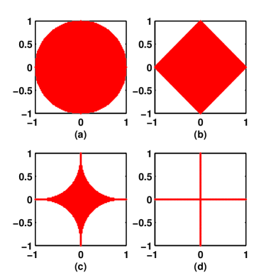
Fig. 1: The geometries of $l_{p}$ norm: (a) $p=2$; (b) $p=1$; (c) $p=0.5$; (d) $p=0$.

Five, can CS have a good performance in a noisy environment? Yes, it can. Because the recovery algorithm can get the most important $K$ components and force other components (including noise components) to be zero. For the image processing, the recovery algorithm will not smooth the image but yield the sharp edge.

Finally, let us review how CS encode and decode the time-domain signal $f$. For the encoder, it gets the measurements $y$ or $\tilde{y}$ according to the observation matrix $\mathcal{M}_{0}$. For the decoder, it recovers $f$ or $\tilde{f}$ by solving the convex optimization problem (1)(2)(3)(4) with $y$ ($\tilde{y}$), $\mathcal{M}_{0}$, and $\Psi$. Hence, CS can be seen as a fast encoder with lower sampling rate (fewer data set). The sampling rate only depends on the sparsity of $f$ in some domains and goes beyond the limit of the Nyquist/Shannon sampling theorem. However, CS will face a challenging problem: How to perfectly recover the signal with low computational complexity and memory?

3 Physics of Compressive Sensing

The most important concepts of the CS theory involve Coherence and Measurement.

In physics, coherence is a property of waves, that enables stationary (i.e. temporally and spatially constant) interference. More generally, coherence describes all correlation properties between physical quantities of a wave. When interfering, two waves can add together to create a larger wave (constructive interference) or subtract from each other to create a smaller wave (destructive interference), depending on their relative phase. The coherence of two waves follows from how well correlated the waves are as quantified by the cross-correlation function. The cross-correlation quantifies the ability to predict the value of the second wave by knowing the value of the first. As an example, consider two waves perfectly correlated for all times. At any time, if the first wave changes, the second will change in the same way. If combined they can exhibit complete constructive interference at all times. It follows that they are perfectly coherent. So, the second wave needs not be a separate entity. It could be the first wave at a different time or position. In this case, sometimes called self-coherence, the measure of correlation is the autocorrelation function. Take the Thomas Young’s double-slit experiment for example, a coherent light source illuminates a thin plate with two parallel slits cut in it, and the light passing through the slits strikes a screen behind them. The wave nature of light causes the light waves passing through both slits to interfere, creating an interference pattern of bright and dark bands on the screen. In fact, the dark bands can relate to the zero components in the signal processing field. It is well known that we select the basis functions coherent with the signal or image. If the signal is the square wave, the haar wavelet is a good choice. If the signal is the sine wave, the Fourier transform is a good choice. The coherence index between a signal and a basis system will decide the sparsity of the signal in the transform-domain. In other words, fewer basis functions will be used or more components in the transform-domain are to be zero if the signal and the basis functions are coherent. For the CS, however, the observation matrix $\mathcal{M}_{0}$ and the time-domain signal $f$ should be incoherent. In addition, the observation matrix $\mathcal{M}_{0}$ and the basis system $\Psi$ also should be incoherent. If it is not the case, the reconstruction matrix $\mathcal{M}_{0}\Psi^{{\dagger}}$ in (5) will be sparse, which violates the UUP theorem.

Then, let us talk about quantum mechanics and the measurement. In physics, a wave function or wavefunction is a mathematical tool used in quantum mechanics to describe any physical system. The values of the wave function are probability amplitudes (complex numbers). The squares of the absolute values of the wave functions $|f|^{2}$ give the probability distribution (the chance of finding the subject at a certain time and position) that the system will be in any of the possible quantum states. The modern usage of the term wave function refers to a complex vector or function, i.e. an element in a complex Hilbert space. An element of a vector space can be expressed in different bases; and so the same applies to wave functions. The components of a wave function describing the same physical state take different complex values depending on the basis being used; however the wave function itself is not dependent on the basis chosen. Similarly, in the signal processing field, we use different basis functions to represent the signal or image.

The quantum state of a system is a mathematical object that fully describes the quantum system. Once the quantum state has been prepared, some aspect of it is measured (for example, its position or energy). It is a postulate of quantum mechanics that all measurements have an associated operator (called an observable operator). The expected result of the measurement is in general described not by a single number, but by a probability distribution that specifies the likelihoods that the various possible results will be obtained. The measurement process is often said to be random and indeterministic. Suppose we take a measurement corresponding to observable operator $\hat{O}$, on a state whose quantum state is $f$. The mean value (expectation value) of the measurement is $\langle f,\hat{O}f\rangle$ and the variance of the measurement is $\langle f,\hat{O}^{2}f\rangle-(\langle f,\hat{O}f\rangle)^{2}$. Each descriptor (mean, variance, etc) of the measurement involves a part of information of the quantum state. In the signal processing field, the observation matrix $\mathcal{M}_{0}$ is a random matrix and each measurement $y_{i}$ captures a portion of information of the signal $f$. Due to the UUP and RIP theorems, all the measurements make the same contribution to recovering $f$. In other words, each measurement $y_{i}$ is equally important or unimportant. The unique property will make CS very powerful in the communication field (channel coding).

4 Gradient-Based Recovery Algorithms

A fast, low-consumed, and reliable recovery algorithm is the core of the CS theory. There are a lot of outstanding work on the topic[7][8][9][10]. Based on their work, we developed the gradient-based recovery algorithms. In particular, we did not reshape the image (matrix) to the signal (vector), which will consume a large amount of memory. We treat each column of the image as a vector and the comparable results also can be obtained. For the sparse image in the time-domain, the $l_{1}$ norm constraint is used. For the general image (especially for the geometric image), the total variation constraint is used. Considering the non-differentiability of the function $|f_{j,k}|$ at the origin point, the subgradient or smooth approximation strategies[10] are employed.

A Gradient Algorithms and Their Geometries

Before solving the constrained convex optimization problems, the clear and deep understandings for the gradient-based algorithms are necessary. Given a linear matrix equation

$$\mathcal{M}_{0}f=y$$ (9)

the solution $f$ can be found by solving the following minimization problem

$$\min_{f}L(f)\equiv\frac{1}{2}||\mathcal{M}_{0}f-y||_{2}^{2}$$ (10)

The gradient-based algorithms for solving (10) can be written as

$$f^{i+1}=f^{i}-\mu^{i}\nabla L(f^{i})$$ (11)

where $\mu^{i}$ is the iteration step size and

$$\nabla L(f^{i})=\mathcal{M}_{0}^{{\dagger}}(\mathcal{M}_{0}f^{i}-y)$$ (12)

A variety of settings for $\mu^{i}$ result in different algorithms involving the gradient method, the steepest descent method, and the Newton’s method. The gradient method sets $\mu^{i}$ to a small constant. The steepest descent method sets $\mu^{i}$ to

$$\mu^{i}=\frac{\left\langle\nabla L(f^{i}),\nabla L(f^{i})\right\rangle}{\left\langle\nabla L(f^{i}),\mathcal{M}_{0}^{{\dagger}}\mathcal{M}_{0}\nabla L(f^{i})\right\rangle+\varepsilon}$$ (13)

which minimizes the residual $R^{i}=\mathcal{M}_{0}f^{i}-y$ in each iteration. Here, the small $\varepsilon$ is used for avoiding a zero denominator. For the Newton’s method, $\mu^{i}$ is taken as a constant matrix

$$\mu^{i}=\left(\mathcal{M}_{0}^{{\dagger}}\mathcal{M}_{0}+\varepsilon I\right)^{-1}$$ (14)

Here, the small $\varepsilon$ is used for avoiding a nearly singular matrix.

To understand the geometries for the three gradient-based algorithms, a simple case is taken for example. A 2-D function $f(x,y)=(x+y)^{2}+(x+1)^{2}+(y+3)^{2}$ has a local minimum $f^{*}=\left(\frac{1}{3},-\frac{5}{3}\right)$. The contour of the function and the trajectory of $f^{i}$ are drawn in Fig. 2.

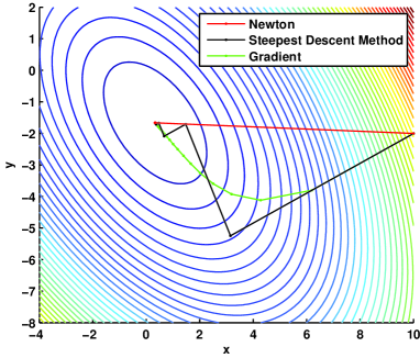
Fig. 2: The geometries for the gradient-based algorithms.

The convergence of the gradient method is worst. The steepest descent method converges fast at the first several steps but slowly as the iteration step increases. The Newton’s method is best and needs only one step for the 2-D case.

Next, we will apply the steepest descent method and the Newton’s method to recover the signal or image $f$ by using (1). The treatments for other convex optimization problems (2)(3)(4) are similar.

B $l_{1}$ Norm Strategy

We assume $f_{j,k}$ is the pixel of an $N\times N$ image $f$ at the j-th row and the k-th column ($1\leq j\leq N$ and $1\leq k\leq N$). The convex optimization problem (1) for the sparse image can be converted to

$$\min_{f}H(f)\equiv L(f)+\lambda\|f\|_{1}$$ (15)

where $\|f\|_{1}=\sum_{j,k}|f_{j,k}|$. The above equation is a Lagrange multiplier formulation. The first term relates to the underdetermined matrix equation (9) and the second $l_{1}$-penalty term will assure a regularized sparse solution. The parameter $\lambda$ balances the weight of the first term and the second term.

Because $|f_{j,k}|$ is not differentiable at the origin point, we can define a new subgradient for each $f_{j,k}$ as follows

$$\nabla_{j,k}{H(f)}=\left\{\begin{array}[]{cl}&\nabla_{j,k}{L(f)}+\lambda\,\mathrm{sign}(f_{j,k}),\,\,|f_{j,k}|\geq\varepsilon\\ &\nabla_{j,k}L(f)+\lambda,\,\,|f_{j,k}|<\varepsilon,\,\,\nabla_{j,k}L(f)<-\lambda\\ &\nabla_{j,k}L(f)-\lambda,\,\,|f_{j,k}|<\varepsilon,\,\,\nabla_{j,k}L(f)>\lambda\\ &0,\,\,|f_{j,k}|<\varepsilon,\,\,\left|\nabla_{j,k}L(f)\right|\leq\lambda\end{array}\right.$$ (20)

Then the gradient-based algorithm can be written as

$$f_{j,k}^{i+1}=f_{j,k}^{i}-\mu_{k}^{i}\nabla_{j,k}H(f^{i})$$ (21)

where $j$ and $k$ are, respectively, the row index and the column index of the image $f$ and $i$ denotes the i-th iteration step. The $\mu_{k}^{i}$ has been given in (13) and (14). Bear in mind, the image will be treated column by column when computing $\mu_{k}^{i}$ and $\nabla_{j,k}{L(f^{i})}$.

For the steepest descent method, the parameter $\lambda$ can be taken as a small positive constant ($\lambda=0.001-0.01$). But for the Newton’s method, the parameter $\lambda$ must be gradually decreased as the iteration step increases ($\lambda^{i+1}=(0.99-0.999)\times\lambda^{i}$).

C Total Variation Strategy

For a general image, especially for a geometric image, it is not sparse in the time-domain. Hence, the $l_{1}$ norm strategy developed in the previous subsection will break down.

The convex optimization problem for the general image can be given by

$$\min_{f}H(f)\equiv L(f)+\lambda\,\rm{TV}(f)$$ (22)

where $\rm{TV}(f)$ is the total variation of the image $f$. The derivatives of $f$ along the vertical and horizontal directions can be defined as

$$D_{j,k}^{v}f=\left\{\begin{array}[]{lc}f_{j,k}-f_{j+1,k}&1\leq j<N\\ 0&j=N\end{array}\right.$$ (25)

$$D_{j,k}^{h}f=\left\{\begin{array}[]{lc}f_{j,k}-f_{j,k+1}&1\leq k<N\\ 0&k=N\end{array}\right.$$ (28)

The total variation of the image $f$ is the summation for the magnitude of the gradient of each pixel [11]

$$\rm{TV}(f)=\sum_{j,k}{\sqrt{\left(D_{j,k}^{v}f\right)^{2}+\left(D_{j,k}^{h}f\right)^{2}}}=\sum_{j,k}\left|\nabla_{j,k}f\right|$$ (29)

After some simple derivations, the gradient of the total variation with each pixel is given by

$$\begin{split}\nabla_{j,k}\left(\rm{TV}(f)\right)&=\frac{D_{j,k}^{v}f}{\left|\nabla_{j,k}f\right|}+\frac{D_{j,k}^{h}f}{\left|\nabla_{j,k}f\right|}\\ &-\frac{D_{j-1,k}^{v}f}{\left|\nabla_{j-1,k}f\right|}-\frac{D_{j,k-1}^{h}f}{\left|\nabla_{j,k-1}f\right|}\end{split}$$ (30)

When treating (30), the smooth approximation strategy is used for avoiding a zero denominator, i.e.

$$\left|\nabla_{j,k}f\right|=\sqrt{\left(D_{j,k}^{v}f\right)^{2}+\left(D_{j,k}^{h}f\right)^{2}+\varepsilon}$$ (31)

The gradient-based algorithm has been given in (21).

5 Numerical Experiments and Results

A Cases of $l_{1}$ Norm Strategy

The first image we’d like to recover is a $64\times 64$ sparse diamond as shown in Fig. 3.

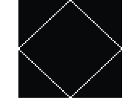
Fig. 3: The $64\times 64$ sparse diamond.

Notice that the image itself is sparse in the time-domain, we need not to transform the image into other domains, such as the wavelet domain or Fourier domain. The size of the observation matrix for the nearly perfect reconstruction should be at least larger than $12\times 64$ where $12$ is calculated by $2\cdot\log_{2}{64}=12$. If our observation matrices are generated by the uniform distribution from $0$ to $1$, after $20000$ iteration steps, Fig. 4 can be obtained. The subplot (a) shows the recovered image with a $10\times 64$ observation matrix, while (b), (c), and (d) are recovered with $12\times 64$, $15\times 64$, and $20\times 64$ random observation matrices respectively. When the size of the observation matrix is small, the poor reconstructed images are shown in (a) and (b). But when the observation matrix gets larger and larger, the better results can be obtained as shown in (c) and (d).

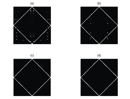
Fig. 4: The recovered diamond figures by the Newton’s method from the observation matrices with different sizes: (a) $10\times 64$; (b) $12\times 64$; (c) $15\times 64$; (d) $20\times 64$.

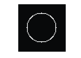
Fig. 5: The $64\times 64$ sparse circle.

Another $64\times 64$ image we wish to recover is a circle as shown in Fig. 5. Although the circle is sparse on the whole, but it is not the case for some columns. These columns may require more measurements if we treat an $n\times n$ image as $n$ vectors. Using the steepest descent method, we can recover the image after several iterations. Here, we don’t want to compare the Newton’s method with the steepest descent method to find which one is more powerful and effective. (Actually, their performances are almost the same for the image.) What we want to show is the sparsity of an image affects the recovered results a lot. Fig. 6 shows the recovered results from the observation matrices with different sizes slightly larger than the previous case. For the subplots (a) and (b), the results are undesirable. The subplot (c) is better and almost perfect reconstruction is obtained for the subplot (d). Again, we notice that for the small observation matrix, the recovered results may vary drastically. If the size of the observation matrix is large enough, the reconstructed image is accurate or even exact in any repeated experiments. The subplots (a), (b), and (c) in Fig. 6 show that those columns which are less sparse are the hardest to recover when the small observation matrix is utilized. For the case, the total variation strategy may be a better choice. In a word, a large observation matrix can capture more information of the image and therefore the image can be recovered with higher probability.

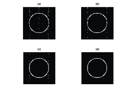
Fig. 6: The recovered circle figures by the steepest descent method from the observation matrices with different sizes: (a) $15\times 64$; (b) $20\times 64$; (c) $25\times 64$; (d) $30\times 64$.

B Cases of Total Variation Strategy

If the image is not sparse in the time-domain, it also can be recovered from the measurements without represented as the basis functions $\Psi$ whose coefficients may be sparse. For instance, the geometric figure composed of a solid circle and a solid square is shown in Fig. 7. It is easy to imagine the derivatives of the image are sparse. We apply the total variation strategy to recover the image.

Fig. 7: The geometric figure.

The size of the object image again is $64\times 64$ and the $20\times 64$ observation matrix is employed. Fig. 8 is the typical measurements $y$ and Fig.  9 is the reconstructed image from $y$. The peak signal to noise ratio (PSNR) calculated is always above $90$ for the repeated experiments (different observation matrices with the same size), which suggests that the observation matrix is large enough to recover the original image with an extremely accurate result.

Fig. 8: The measurement of the geometric figure.

Fig. 9: The recovered geometric image by the steepest descent method: $20\times 64$ observation matrix is employed.

The next two images Cameraman and Boats in Fig. 10 are quite well-known in the image processing field. We still treat the $256\times 256$ image as $256$ vectors. Although the result may not be so good as that we obtain by treating the $256\times 256$ image as a long vector of size $65536\times 1$, we do save a great amount of memory and calculation time. The size of our observation matrix $\mathcal{M}_{0}$ is $100\times 256$ rather than $25600\times 65536$ ($25600\approx 65536/2.56$). The recovery algorithm is implemented in the wavelet-domain, and the PSNR for the subplots (a) and (b) in Fig. 11 are $29.4$ and $30.9$, respectively. In addition, the gradient-based total variation algorithm also has a good performance for the geometric image Peppers. (Showing too many results are not necessary).

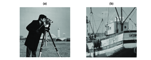
Fig. 10: The general image: (a) Cameraman; (b) Boats.

Fig. 11: The recovered images by the Newton’s method: $100\times 256$ observation matrix is employed. (a) Cameraman; (b) Boats.

6 Discussions and Future Work

The above are just some simple experiments for demonstrating that the CS was able to recover an image accurately from a few of random projections. One should understand that the main advantage of CS is not how small size it can compress the image to. In fact, if a signal is $K$ sparse in some domains, we indeed require $3K$ to $5K$ measurements to recover the signal. An obvious advantage of CS is that it can encode the signal or image fast. In particular, the prior knowledge about the signal is not important. For example, it is not necessary for us to know the exact positions and values of the most important components beforehand. What we care is whether the image is sparse in some domains or not. A fixed observation matrix can be applied to measure different signals, which makes the applications of CS for encoding and decoding possible. Meanwhile, the measurements play the same role in recovering the signal or image, which makes CS very powerful in military applications (radar imaging) where we cannot afford the risk caused by the loss of the most important $K$ components. Since each random projection (measurement) is equally (un)important, the CS is not sensitive to the noises or measurement errors and can provide the robust and stable performances.

Although many researchers have made great progresses in the convex optimization problems and demonstrated the accurate results on the scale we interest (hundreds of thousands of measurements and millions of pixels), the more efficient algorithms are still required. Actually, solving the $l_{1}$ minimization problem is about 30-50 times as expensive as solving the least squares problem. However, the unbalanced computational burden gives us a chance that the measurements are acquired by the sensors with lower power, and then the signal or image will be recovered on the central supercomputer. The algorithms, such as the conjugate gradient method and the generalized minimal residual method, will become our next candidates for accelerating the recovery algorithm.

The physical understandings and applications for CS are under way, although a single-pixel camera has shocked the field of optics. We are aware that the CS has penetrated many fields and become a hotspot. We expect more mathematicians, physicist, and engineers make contributions for the CS field.

7 Acknowledgement

The authors are not from signal or image processing society. Hence, some technical words may not be right. We hope the report can give some help for the researchers form the signal processing, image processing, and physical societies.

References

- [1] Emmanuel J. Candès, Justin K. Romberg, and Terence Tao, “Robust uncertainty principles: Exact signal reconstruction from highly incomplete frequency information,” IEEE Transactions On Information Theory, vol. 52, pp. 489-509, Feb. 2006.
- [2] David L. Donoho, “Compressed sensing,” IEEE Transactions On Information Theory, vol. 52, pp. 1289-1306, Apr. 2006.
- [3] Emmanuel J. Candès and Michael B. Wakin, “People hearing without listening:” An introduction to compressive sampling, Report.
- [4] Richard G. Baraniuk, “Compressive sensing,” IEEE Signal Processing Magazine, pp. 118-124, Jul. 2007.
- [5] Emmanuel J. Candès and Michael B. Wakin, “An introduction to compressive sampling,” IEEE Signal Processing Magazine, pp. 21-230, Mar. 2008.
- [6] Justin K. Romberg, “Imaging via compressive sampling,” IEEE Signal Processing Magazine, pp. 14-20, Mar. 2008.
- [7] Emmanuel J. Candès and Justin K. Romberg, “Signal recovery from random projections,” Proceedings of SPIE-IS&T Electronic Imaging, vol. 5674, pp. 76-86, Mar. 2005.
- [8] Emmanuel J. Candès and Terence Tao, “Decoding by linear programming,” IEEE Transactions On Information Theory, vol. 51, pp. 4203-4215, Dec. 2005.
- [9] Joel A. Tropp and Anna C. Gilbert, “Signal recovery from partial information via orthogonal matching pursuit,” IEEE Transactions On Information Theory, vol. 53, pp. 4655-4666, Dec. 2007.
- [10] Mark Schmidt, Glenn Fung, and Rómer Rosales, Fast optimization methods for L1 regularization: A comparative study and two new approaches, Machine Learning: ECML 2007, vol. 4701, Sep. 2007.
- [11] Leonid I. Rudin, Stanley Osher, and Emad Fatemi, “Nonlinear total variation based noise removal algorithms,” Physica D, vol. 60, pp. 259-268, Nov. 1992.