Well-posed elliptic Neumann problems
involving irregular data and domains

Abstract

Nonlinear elliptic Neumann problems, possibly in irregular domains and with data affected by low integrability properties, are taken into account. Existence, uniqueness and continuous dependence on the data of generalized solutions are established under a suitable balance between the integrability of the datum and the (ir)regularity of the domain. The latter is described in terms of isocapacitary inequalities. Applications to various classes of domains are also presented.

Résumé

Nous considérons des problèmes de Neumann pour des équations elliptiques non linéaires dans domaines éventuellement non réguliers et avec des données peu régulières. Un équilibre entre l’intégrabilité de la donnée et l’(ir)régularité du domaine nous permet d’obtenir l’existence, l’unicité et la dépendance continue de solutions généralisées. L’irrégularité du domaine est décrite par des inegalités “isocapacitaires”. Nous donnons aussi des applications à certaines classes de domaines.

1 Introduction and main results

The present paper deals with existence, uniqueness and continuous dependence on the data of solutions to nonlinear elliptic Neumann problems having the form

(1.1) $$\begin{cases}-{\rm div}(a(x,\nabla u))=f(x)&{\rm in}\,\,\,\Omega\\ a(x,\nabla u)\cdot{\bf n}=0&{\rm on}\,\,\,\partial\Omega\,.\end{cases}$$

Here:

$\Omega$ is a connected open set in ${{\mathbb{R}}^{n}}$, $n\geq 2$, having finite Lebesgue measure $|\Omega|$;

$a~{}:~{}\Omega~{}\times~{}{{\mathbb{R}}^{n}}~{}\rightarrow~{}{{\mathbb{R}}^{n}}$ is a Carathéodory function;

$f\in L^{q}(\Omega)$ for some $q\in[1,\infty]$ and satisfies the compatibility condition

(1.2) $$\int_{\Omega}f(x)dx=0.$$

Moreover, $``\cdot"$ stands for inner product in ${{\mathbb{R}}^{n}}$, and ${\bf n}$ denotes the outward unit normal on $\partial\Omega$.

Standard assumptions in the theory of nonlinear elliptic partial differential equations amount to requiring that there exist an exponent $p>1$, a function $h\in L^{p^{\prime}}(\Omega)$, where $p^{\prime}=\frac{p}{p-1}$, and a constant $C$ such that, for a.e. $x\in\Omega$ :

(1.3) $$a(x,\xi)\cdot\xi\geq|\xi|^{p}\quad\hbox{for}\,\,\,\xi\in{{\mathbb{R}}^{n}}\,;$$

(1.4) $$|a(x,\xi)|\leq C(|\xi|^{p-1}+h(x))\quad\hbox{for}\,\,\,\xi\in{{\mathbb{R}}^{n}}\,;$$

(1.5) $$[a(x,\xi)-a(x,\eta)]\cdot(\xi-\eta)>0\quad\hbox{for}\,\,\,\xi,\eta\in{{\mathbb{R}}^{n}}\,\,\,\hbox{with}\,\,\,\xi\neq\eta\,.$$

The $p$-Laplace equation, corresponding to the choice $a(x,\xi)=|\xi|^{p-2}\xi$, and, in particular, the (linear) Laplace equation when $p=2$, can be regarded as prototypal examples on which our analysis provides new results.

When $\Omega$ is sufficiently regular, say with a Lipschitz boundary, and $q$ is so large that $f$ belongs to the topological dual of the classical Sobolev space $W^{1,p}(\Omega)$, namely $q>\frac{np}{np-n+p}$ if $p<n$, $q>1$ if $p=n$, and $q\geq 1$ if $p>n$, the existence of a unique (up to additive constants) weak solution to problem (1.1) under (1.2)-(1.5) is well known, and quite easily follows via the Browder-Minthy theory of monotone operators.

In the present paper, problem (1.1) will be set in a more general framework, where these customary assumptions on $\Omega$ and $f$ need not be satisfied. Of course, solutions to (1.1) have to be interpreted in an extended sense in this case. The notion of solution $u$, called approximable solution throughout this paper, that will be adopted arises quite naturally in dealing with problems involving irregular domains and data. Loosely speaking, it amounts to demanding that $u$ be a distributional solution to (1.1) which can be approximated by a sequence of solutions to problems with the same differential operator and boundary condition, but with regular right-hand sides. A precise definition can be found in Section 2.3. We just anticipate here that an approximable solution $u$ need not be a Sobolev function in the usual sense; nevertheless, a generalized meaning to its gradient $\nabla u$ can be given.

Definitions of solutions of this kind, and other definitions which, a posteriori, turn out to be equivalent, have been extensively employed in the study of elliptic Dirichlet problems with a right-hand side $f$ affected by low integrability properties. Initiated in [Ma2, Ma3] and [St] in the linear case, and in [BG1, BG2] in the nonlinear case, this study has been the object of several contributions in the last twenty years, including [AM, BBGGPV, DaA, DM, DMOP, De, LM, M1, M2, DHM, GIS, FS]. These investigations have pointed out that, when dealing with (homogeneous) Dirichlet boundary conditions, existence and uniqueness of solutions can be established as soon as $f\in L^{1}(\Omega)$, whatever $\Omega$ is. In fact, the regularity of $\Omega$ does not play any role in this case, the underlying reason being that the level sets of solutions cannot reach $\partial\Omega$.

The situation is different when Neumann boundary conditions are prescribed. Actually, inasmuch as the boundary of the level sets of solutions and $\partial\Omega$ can actually overlap, the geometry of the domain $\Omega$ comes now into play. We shall prove that problem (1.1) is still uniquely solvable, provided that the (ir)regularity of $\Omega$ and the integrability of $f$ are properly balanced. In fact, even if $f$ highly integrable, in particular essentially bounded, some regularity on $\Omega$ has nevertheless to be retained. In the special case when $\Omega$ is smooth, or at least with a Lipschitz boundary, our results overlap with contributions from [AMST, BeGu, Dr, DV, Po, Pr, DLR].

Our approach relies upon isocapacitary inequalities, which have recently been shown in [CM1] to provide suitable information on the regularity of the domain $\Omega$ in the study of problems of the form (1.1). In fact, isocapacitary inequalities turn out to be more effective than the more popular isoperimetric inequalities in this kind of applications. The use of the standard isoperimetric inequality in the study of elliptic Dirichlet problems, and of relative isoperimetric inequalities in the study of Neumann problems, was introduced in [Ma2, Ma3]. The isoperimetric inequality was also independently employed in [Ta1, Ta2] in the proof of symmetrization principles for solutions to Dirichlet problems. Ideas from these papers have been developed in a rich literature, including [Al, AFLT, ALT, Ke1]. Specific contributions to the study of Neumann problems are [AMT, Be, Ci2, A.Fe, V.Fe1, MS1, MS2]. We refer to [Ke2, Tr, Va] for an exhaustive bibliography on these topics.

The relative isoperimetric inequality in $\Omega$ tells us that

(1.6) $$\lambda(|E|)\leq P(E;\Omega)\qquad\quad\hbox{for every measurable set $E\subset\Omega$ with $|E|\leq|\Omega|/2$},$$

where $P(E;\Omega)$ denotes the perimeter of a measurable set $E$ relative to $\Omega$, and $\lambda:[0,|\Omega|/2]\rightarrow[0,\infty)$ is the isoperimetric function of $\Omega$.

Replacing the relative perimeter by a suitable $p$-capacity on the right-hand side of (1.6) leads to the isocapacitary inequality in $\Omega$. Such inequality reads

(1.7) $$\nu_{p}(|E|)\leq C_{p}(E,G)\quad\hbox{for every measurable sets $E\subset G\subset\Omega$ with $|G|\leq|\Omega|/2$},$$

where $C_{p}(E,G)$ is the $p$-capacity of the condenser $(E;G)$ relative to $\Omega$, and ${\nu_{p}}:[0,|\Omega|/2]\rightarrow[0,\infty]$ is the isocapacitary function of $\Omega$.

Precise definitions concerning perimeter and capacity, together with their properties entering in our discussion, are given in Section 2.4. Let us emphasize that although (1.6) and (1.7) are essentially equivalent for sufficiently smooth domains $\Omega$, the isocapacitary inequality (1.7) offers, in general, a finer description of the regularity of bad domains $\Omega$. Accordingly, our main results will be formulated and proved in terms of the function $\nu_{p}$. Their counterparts involving $\lambda$ will be derived as corollaries - see Section 5. Special instances of bad domains and data will demonstrate that the use of $\nu_{p}$ instead of $\lambda$ can actually lead to stronger conclusions in connection with existence, uniqueness and continuous dependence on the data of solutions to problem (1.1).

Roughly speaking, the faster the function $\nu_{p}(s)$ decays to $0$ as $s\to 0^{+}$, the worse is the domain $\Omega$, and, obviously, the smaller is $q$, the worse is $f$. Accordingly, the spirit of our results is that problem (1.1) is actually well-posed, provided that $\nu_{p}(s)$ does not decay to $0$ too fast as $s\to 0^{+}$, depending on how small $q$ is. Our first theorem provides us with conditions for the unique solvability (up to additive constants) of (1.1) under the basic assumptions (1.2)–(1.5).

Theorem 1.1

Let $\Omega$ be an open connected subset of ${{\mathbb{R}}^{n}}$, $n\geq 2$, having finite measure. Assume that $f\in L^{q}(\Omega)$ for some $q\in[1,\infty]$ and satisfies (1.2). Assume that (1.3)-(1.5) are fulfilled, and that either

(i) $1<q\leq\infty$ and

(1.8) $$\int_{0}^{|\Omega|/2}\bigg{(}\frac{s}{\nu_{p}(s)}\bigg{)}^{\frac{q^{\prime}}{p}}ds<\infty\,,$$

or

(ii) $q=1$ and

(1.9) $$\int_{0}^{|\Omega|/2}\bigg{(}\frac{s}{\nu_{p}(s)}\bigg{)}^{\frac{1}{p}}\frac{ds}{s}<\infty\,.$$

Then there exists a unique (up to additive constants) approximable solution to problem (1.1).

The second main result of this paper is concerned with the case when the differential operator in (1.1) is not merely strictly monotone in the sense of (1.5), but fulfils the strong monotonicity assumption that, for a.e. $x\in\Omega$,

(1.10) $$[a(x,\xi)-a(x,\eta)]\cdot(\xi-\eta)\geq\begin{cases}C|\xi-\eta|^{p}&{\rm if}\,\,\,p\geq 2\\ C\displaystyle{\frac{|\xi-\eta|^{2}}{(|\xi|+|\eta|)^{2-p}}}&{\rm if}\,\,\,1<p<2\,,\end{cases}$$

for some positive constant $C$ and for $\xi,\eta\in{{\mathbb{R}}^{n}}$. In addition to the result of Theorem 1.1, the continuous dependence of the solution to (1.1) with respect to $f$ can be established under the reinforcement of (1.5) given by (1.10). In fact, when (1.10) is in force, a partially different approach can be employed, which also simplifies the proof of the statement of Theorem 1.1.

Observe that, in particular, assumption (1.10) certainly holds provided that, for a.e. $x\in\Omega$, the function $a(x,\xi)=(a_{1}(x,\xi),\dots,a_{n}(x,\xi))$ is differentiable with respect to $\xi$, vanishes for $\xi=0$, and satisfies the ellipticity condition

$$\sum_{i,j=1}^{n}\frac{\partial a_{i}}{\partial\xi_{j}}(x,\xi)\eta_{i}\eta_{j}\geq C|\xi|^{p-2}|\eta|^{2}\qquad\hbox{for $\xi,\eta\in{{\mathbb{R}}^{n}}$},$$

for some positive constant $C$.

Theorem 1.2

Let $\Omega$, $p$, $q$ and $f$ be as in Theorem 1.1. Assume that (1.3), (1.4) and (1.10) are fulfilled. Assume that either $1<q\leq\infty$ and (1.8) holds, or $q=1$ and (1.9) holds.

Then there exists a unique (up to additive constants) approximable solution to problem (1.1) depending continuously on the right-hand side of the equation. Precisely, if $g$ is another function from $L^{q}(\Omega)$ such that $\int_{\Omega}g(x)dx=0$, and $v$ is the solution to (1.1) with $f$ replaced by $g$, then

(1.11) $$\|\nabla u-\nabla v\|_{L^{p-1}(\Omega)}\leq C\|f-g\|_{L^{q}(\Omega)}^{\frac{1}{r}}\big{(}\|f\|_{L^{q}(\Omega)}+\|g\|_{L^{q}(\Omega)}\big{)}^{\frac{1}{p-1}-\frac{1}{r}}$$

for some constant $C$ depending on $p$, $q$ and on the left-hand side either of (1.8) or (1.9). Here, $r=\max\{p,2\}$.

Let us notice that the balance condition between $q$ and $\nu_{p}$ in Theorems 1.1 and 1.2 requires a separate formulation according to whether $q>1$ or $q=1$. In fact, assumption (1.9) is a qualified version of the limit as $q\to 1^{+}$ of (1.8). This is as a consequence of the different a priori (and continuous dependence) estimates upon which Theorems 1.1 and 1.2 rely. Actually, $L^{1}(\Omega)$ is a borderline space, and when $f\in L^{1}(\Omega)$ the natural sharp estimate involves a weak type (i.e. Marcinkiewicz) norm of the gradient of the solution $u$. Instead, when $f\in L^{q}(\Omega)$ with $q>1$, a strong type (i.e. Lebesgue) norm comes into play in a sharp bound for the gradient of $u$. This gap is intrinsic in the problem, as witnessed by the basic case of the Laplace (or p-Laplace) operator in a smooth domain.

The paper is organized as follows. In Section 2 we collect definitions and basic properties concerning functions spaces of measurable (Subsection 2.1) and weakly differentiable functions (Subsection 2.2), solutions to problem (1.1) (Subsection 2.3), perimeter and capacity (Subsection 2.4). Section 3 is devoted to the proof of Theorem 1.1, which is accomplished in Subsection 3.2, after deriving the necessary a priori estimates in Subsection 3.1. Continuous dependence estimates under the strong monotonicity assumption (1.10) are established in Subsection 4.1 of Section 4; they are a key step in the proof of Theorem 1.2 given in Subsection 4.2. Finally, Section 5 contains applications of our results to special domains and classes of domains. Versions of Theorems 1.1 and 1.2 involving the isoperimetric function are also preliminarily stated. With their help, the advantage of the use of isocapacitary inequalities instead of isoperimetric inequalities is demonstrated in concrete examples.

2 Background and preliminaries

2.1 Rearrangements and rearrangement invariant spaces

Let us denote by $\mathcal{M}(\Omega)$ the set of measurable functions in $\Omega$, and let $u\in\mathcal{M}(\Omega)$. The distribution function $\mu_{u}:[0,\infty)\rightarrow[0,\infty)$ of $u$ is defined as

(2.1) $$\mu_{u}(t)=|\{x\in\Omega:|u(x)|\geq t\}|,\qquad\hbox{for $t\geq 0$}.$$

The decreasing rearrangement $u^{*}:[0,|\Omega|]\rightarrow[0,\infty]$ of $u$ is given by

(2.2) $$u^{*}(s)=\sup\,\{t\geq 0:\mu_{u}(t)\geq s\}|,\qquad\hbox{for }s\in[0,|\Omega|].$$

We also define $u_{*}:[0,|\Omega|]\rightarrow[0,\infty]$, the increasing rearrangement of $u$, as

$$u_{*}(s)=u^{*}(|\Omega|-s),\qquad\hbox{for }s\in[0,|\Omega|].$$

The operation of decreasing rearrangement is neither additive nor subadditive. However,

(2.3) $$(u+v)^{*}(s)\leq u^{*}(s/2)+v^{*}(s/2),\qquad\hbox{for }s\in[0,|\Omega|],$$

for any $u,v\in\mathcal{M}(\Omega)$, and hence, via Young’s inequality,

(2.4) $$(uv)^{*}(s)\leq u^{*}(s/2)v^{*}(s/2),\qquad\hbox{for }s\in[0,|\Omega|].$$

A basic property of rearrangements is the Hardy-Littlewood inequality, which tells us that

(2.5) $$\int_{0}^{|\Omega|}u^{*}(s)v_{*}(s)\,ds\leq\int_{\Omega}|u(x)v(x)|\,dx\leq\int_{0}^{|\Omega|}u^{*}(s)v^{*}(s)\,ds\$$

for any $u,v\in\mathcal{M}(\Omega)$.

A rearrangement invariant (r.i., for short) space $X(\Omega)$ on $\Omega$ is a Banach function space, in the sense of Luxemburg, equipped with a norm $\|\cdot\|_{X(\Omega)}$ such that

(2.6) $$\|u\|_{X(\Omega)}=\|v\|_{X(\Omega)}\qquad\quad\hbox{whenever $u^{*}=v^{*}$}.$$

Since we are assuming that $|\Omega|<\infty$, any r.i. space $X(\Omega)$ fulfills

$$L^{\infty}(\Omega)\to X(\Omega)\to L^{1}(\Omega)\,,$$

where the arrow “$\to$” stands for continuous embedding.

Given any r.i. space $X(\Omega)$, there exists a unique r.i. space $\overline{X}(0,|\Omega|)$, the representation space of $X(\Omega)$ on $(0,|\Omega|)$, such that

(2.7) $$\|u\|_{X(\Omega)}=\|u^{*}\|_{\overline{X}(0,|\Omega|)}$$

for every $u\in X(\Omega)$. A characterization of the norm $\|\cdot\|_{\overline{X}(0,|\Omega|)}$ is available (see [BS, Chapter 2, Theorem 4.10 and subsequent remarks]). However, in our applications, an expression for $\overline{X}(0,|\Omega|)$ will be immediately derived via basic properties of rearrangements. In fact, besides the standard Lebesgue spaces, we shall only be concerned with Lorentz and Marcinkiewicz type spaces. Recall that, given $\sigma,\varrho\in(0,\infty)$, the Lorentz space $L^{\sigma,\varrho}(\Omega)$ is the set of all functions $u\in\mathcal{M}(\Omega)$ such that the quantity

(2.8) $$\|u\|_{L^{\sigma,\varrho}(\Omega)}=\left(\int_{0}^{|\Omega|}(s^{\frac{1}{\sigma}}u^{*}(s))^{\varrho}\frac{ds}{s}\right)^{1/\varrho}$$

is finite. The expression $\|\cdot\|_{L^{\sigma,\varrho}(\Omega)}$ is an (r.i.) norm if and only if $1\leq\varrho\leq\sigma$. When $\sigma\in(1,\infty)$ and $\varrho\in[1,\infty)$, it is always equivalent to the norm obtained on replacing $u^{*}(s)$ by $\frac{1}{s}\int_{0}^{s}u^{*}(r)dr$ on the right-hand side of (2.8); the space $L^{\sigma,\varrho}(\Omega)$, endowed with the resulting norm, is an r.i. space. Note that $L^{\sigma,\sigma}(\Omega)=L^{\sigma}(\Omega)$ for $\sigma>0$. Moreover, $L^{\sigma,\varrho_{1}}(\Omega)\subsetneqq L^{\sigma,\varrho_{2}}(\Omega)$ if $\varrho_{1}<\varrho_{2}$, and, since $|\Omega|<\infty$, $L^{\sigma_{1},\varrho_{1}}(\Omega)\subsetneqq L^{\sigma_{2},\varrho_{2}}(\Omega)$ if $\sigma_{1}>\sigma_{2}$ and $\varrho_{1},\varrho_{2}\in(0,\infty].$

Let $\omega:(0,|\Omega|)\rightarrow(0,\infty)$ be a bounded non-decreasing function. The Marcinkiewicz space $M_{\omega}(\Omega)$ associated with $\omega$ is the set of all functions $u\in\mathcal{M}(\Omega)$ such that the quantity

(2.9) $$\|u\|_{M_{\omega}(\Omega)}=\sup_{s\in(0,|\Omega|)}\omega(s)u^{*}(s)$$

is finite. The expression (2.9) is equivalent to a norm, which makes $M_{\omega}(\Omega)$ an r.i. space, if and only if $\sup_{s\in(0,|\Omega|)}\frac{\omega(s)}{s}\int_{0}^{s}\frac{dr}{\omega(r)}<\infty$ .

2.2 Spaces of Sobolev type

Given any $p\in[1,\infty]$, we denote by $W^{1,p}(\Omega)$ the standard Sobolev space, namely

$$W^{1,p}(\Omega)=\{u\in L^{p}(\Omega):\,\,\hbox{$u$ is weakly differentiable in $\Omega$ and $|\nabla u|\in L^{p}(\Omega)$}\}.$$

The space $W_{loc}^{1,p}(\Omega)$ is defined analogously, on replacing $L^{p}(\Omega)$ by $L_{loc}^{p}(\Omega)$ on the right-hand side.

Given any $t>0$, let $T_{t}:\mathbb{R}\rightarrow\mathbb{R}$ be the function given by

(2.10) $$T_{t}(s)=\begin{cases}s&{\rm if}\,\,\,|s|\leq t\\ t\,{\rm sign}(s)&{\rm if}\,\,\,|s|>t\,.\end{cases}$$

For $p\in[1,\infty]$, we set

(2.11) $$W^{1,p}_{T}(\Omega)=\left\{u:\hbox{$u\in\mathcal{M}(\Omega)$ and $T_{t}(u)\in W^{1,p}(\Omega)$ for every $t>0$}\right\}\,.$$

The space $W_{T,loc}^{1,p}(\Omega)$ is defined accordingly, on replacing $W^{1,p}(\Omega)$ by $W_{loc}^{1,p}(\Omega)$ on the right-hand side of (2.11). If $u\in W_{T,loc}^{1,p}(\Omega)$, there exists a (unique) measurable function $Z_{u}:\Omega\to{{\mathbb{R}}^{n}}$ such that

(2.12) $$\nabla\big{(}T_{t}(u)\big{)}=\chi_{\{|u|<k\}}Z_{u}\qquad\quad\hbox{a.e. in $\Omega$}$$

for every $t>0$ [BBGGPV, Lemma 2.1]. Here $\chi_{E}$ denotes the characteristic function of the set $E$. One has that $u\in W_{loc}^{1,p}(\Omega)$ if and only if $u\in W_{T,loc}^{1,p}(\Omega)\cap L_{loc}^{p}(\Omega)$ and $Z_{u}\in L_{loc}^{p}(\Omega,{{\mathbb{R}}^{n}})$, and, in this case, $Z_{u}=\nabla u$. An analogous property holds provided that “loc” is dropped everywhere. In what follows, with abuse of notation, for every $u\in W_{T,loc}^{1,p}(\Omega)$ we denote $Z_{u}$ by $\nabla u$.

Given $p\in(0,\infty]$, define

$$V^{1,p}(\Omega)=\left\{u:u\in W_{T,loc}^{1,1}(\Omega)\hbox{ and }|\nabla u|\in L^{p}(\Omega)\right\}\,.$$

Note that, if $p\geq 1$, then

$$V^{1,p}(\Omega)=\left\{u:u\in W_{loc}^{1,1}(\Omega)\hbox{ and }|\nabla u|\in L^{p}(\Omega)\right\}\,,$$

a customary space of weakly differentiable functions. Moreover, if $p\geq 1$, the set $\Omega$ is connected, and $B$ is any ball such that $\overline{B}\subset\Omega$, then $V^{1,p}(\Omega)$ is a Banach space equipped with the norm

$$\|u\|_{V^{1,p}(\Omega)}=\|u\|_{L^{p}(B)}+\|\nabla u\|_{L^{p}(\Omega)}.$$

Note that, replacing $B$ by another ball results an equivalent norm. The topological dual of $V^{1,p}(\Omega)$ will be denoted by $(V^{1,p}(\Omega))^{\prime}$.

Given any ball $B$ as above, define the subspace $V^{1,p}_{B}(\Omega)$ of $V^{1,p}(\Omega)$ as

$$V^{1,p}_{B}(\Omega)=\left\{u\in V^{1,p}(\Omega):\,\,\int_{B}u\,dx=0\right\}\,.$$

Proposition 2.1

Let $p\in[1,\infty]$. Let $\Omega$ be a connected open set in ${{\mathbb{R}}^{n}}$ having finite measure, and let $B$ be any ball such that $\overline{B}\subset\Omega$. Then the quantity

(2.13) $$\|u\|_{V_{B}^{1,p}(\Omega)}=\|\nabla u\|_{L^{p}(\Omega)}$$

defines a norm in $V_{B}^{1,p}(\Omega)$ equivalent to $\|\cdot\|_{V^{1,p}(\Omega)}$. Moreover, if $p\in(1,\infty)$, then $V_{B}^{1,p}(\Omega)$, equipped with this norm, is a separable and reflexive Banach space.

Proof, sketched. The only nontrivial property that has to be checked in order to show that $\|\cdot\|_{V_{B}^{1,p}(\Omega)}$ is actually a norm is the fact that $\|u\|_{V_{B}^{1,p}(\Omega)}=0$ only if $u=0$. This is a consequence of the Poincare type inequality which tells us that, for every smooth open set $\Omega^{\prime}$ such that $\overline{B}\subset\Omega^{\prime}$ and $\overline{\Omega^{\prime}}\subset\Omega$,

(2.14) $$\|u\|_{L^{p}(\Omega^{\prime})}\leq C\|\nabla u\|_{L^{p}(\Omega^{\prime})}\,$$

for some constant $C=C(p,\Omega^{\prime},|B|)$ and for every $u\in V_{B}^{1,p}(\Omega)$ (see e.g. [Zi, Chapter 4]). The same inequality plays a role in showing that $V_{B}^{1,p}(\Omega)$, equipped with the norm $\|\cdot\|_{V_{B}^{1,p}(\Omega)}$, is complete. When $p\in(1,\infty)$, the separability and the reflexivity of $V_{B}^{1,p}(\Omega)$ follow via the same argument as for the standard Sobolev space $W^{1,p}(\Omega)$, on making use of the fact that the map $L:V_{B}^{1,p}(\Omega)\rightarrow(L^{p}(\Omega))^{n}$ given by $Lu=\nabla u$ is an isometry of $V_{B}^{1,p}(\Omega)$ into $(L^{p}(\Omega))^{n}$, and that $(L^{p}(\Omega))^{n}$ is a separable and reflexive Banach space.

2.3 Solutions

When $f\in(V^{1,p}(\Omega))^{\prime}$, and (1.2)–(1.4) are in force, a standard notion of solution to problem (1.1) is that of weak solution. Recall that a function $u\in V^{1,p}(\Omega)$ is called a weak solution to (1.1) if

(2.15) $$\int_{\Omega}a(x,\nabla u)\cdot\nabla\Phi\,dx=\int_{\Omega}f\Phi\,dx\,\qquad\quad\hbox{for every $\Phi\in V^{1,p}(\Omega)$.}$$

An application of the Browder-Minthy theory for monotone operators, resting upon Proposition 2.1, yields the following existence and uniqueness result. The proof can be accomplished along the same lines as in [Ze, Porposition 26.12 and Corollary 26.13]. We omit the details for brevity.

Proposition 2.2

Let $p\in(1,\infty)$ and let $\Omega$ be a bounded connected open set in ${{\mathbb{R}}^{n}}$ having finite measure. If $f\in(V^{1,p}(\Omega))^{\prime}$, then under assumptions (1.2)–(1.5) there exists a unique (up to additive constants) weak solution $u\in V^{1,p}(\Omega)$ to problem (1.1).

The definition of weak solution does not fit the case when $f\notin(V^{1,p}(\Omega))^{\prime}$, since the right-hand side of (2.15) need not be well-defined. This difficulty can be circumvented on restricting the class of test functions $\Phi$ to $W^{1,\infty}(\Omega)$, for instance. This leads to a counterpart, in the Neumann problem setting, of the classical definition of solution to the Dirichlet problem in the sense of distributions. It is however well-known [Se] that such a class of test functions may be too poor for the solution to be uniquely determined, even under an appropriate monotonicity assumption as (1.5).

In order to overcome this drawback, we adopt a definition of solution, in the spirit e.g. of [DaA] and [DM], obtained in the limit from solutions to approximating problems with regular right-hand sides. The idea behind such a definition is that the additional requirement of being approximated by solutions to regular problems identifies a distinguished proper distributional solution to problem (1.1). Specifically, if $\Omega$ is an open set in ${{\mathbb{R}}^{n}}$ having finite measure, and $f\in L^{q}(\Omega)$ for some $q\in[1,\infty]$ and fulfills (1.2), then a function $u\in V^{1,p-1}(\Omega)$ will be called an approximable solution to problem (1.1) under assumptions (1.3) and (1.4) if:

(i)

(2.16) $$\int_{\Omega}a(x,\nabla u)\cdot\nabla\Phi\,dx=\int_{\Omega}f\Phi\,dx\,\qquad\quad\hbox{for every $\Phi\in W^{1,\infty}(\Omega)$,}$$

and

(ii) a sequence $\{f_{k}\}\subset L^{q}(\Omega)\cap(V^{1,p}(\Omega))^{\prime}$ exists such that $\int_{\Omega}f_{k}(x)dx=0$ for $k\in\mathbb{N}$,

$$f_{k}\rightarrow f\qquad\hbox{in $L^{q}(\Omega)$},$$

and the sequence of weak solutions $\{u_{k}\}\subset V^{1,p}(\Omega)$ to problem (1.1), with $f$ replaced by $f_{k}$, satisfies

$$u_{k}\rightarrow u\quad\hbox{ a.e. in $\Omega$}.$$

A few brief comments about this definition are in order. Customary counterparts of such a definition for Dirichlet problems [DaA, DM] just amount to (a suitable version of) property (ii). Actually, the existence of a generalized gradient of the limit function $u$, in the sense of (2.12), and the fact that $u$ is a distributional solution directly follow from analogous properties of the approximating solutions $u_{k}$. This is due to the fact that, whenever $f\in L^{1}(\Omega)$, a priori estimates in suitable Lebesgue spaces for the gradient of approximating solutions to homogeneous Dirichlet problems are available, irrespective of whether $\Omega$ is regular or not. As a consequence, one can pass to the limit in the equations fulfilled by $u_{k}$, and hence infer that $u$ is a distributional solution to the original Dirichlet problem. When Neumann problems are taken into account, the existence of a generalized gradient of $u$ and the validity of (i) is not guaranteed anymore, inasmuch as a priori estimates for $|\nabla u_{k}|$ depend on the regularity of $\Omega$. The membership of $u$ in $V^{1,p-1}(\Omega)$ and equation (i) have consequently to be included as part of the definition of solution.

Let us also mention that the definition of approximable solution can be shown to be equivalent to other definitions patterned on those of entropy solution [BBGGPV] and of renormalized solution [LM] given for Dirichlet problems.

2.4 Perimeter and capacity

The isoperimetric function $\lambda:[0,|\Omega|/2]\to[0,\infty)$ of $\Omega$ is defined as

(2.17) $$\lambda(s)=\inf\{P(E,\Omega):s\leq|E|\leq|\Omega|/2\}\qquad\quad\hbox{for $s\in[0,|\Omega|/2]$}\,.$$

Here, $P(E;\Omega)$ is the perimeter of $E$ relative to $\Omega$, which agrees with ${\cal H}^{n-1}(\partial^{M}E\cap\Omega)$, where ${\cal H}^{n-1}$ denotes the $(n-1)$-dimensional Hausdorff measure, and $\partial^{M}E$ stands for the essential boundary of $E$ (see e.g. [AFP, Ma4]).

The relative isoperimetric inequality (1.6) is a straightforward consequence of definition (2.17). On the other hand, the isoperimetric function $\lambda$ is known only for very special domains, such as balls [Ma4, BuZa] and convex cones [LP]. However, various qualitative and quantitative properties of $\lambda$ have been investigated, in view of applications to Sobolev inequalities [HK, Ma1, Ma4, MP], eigenvalue estimates [Ch, Ci2, Ga], a priori bounds for solutions to Neumann problems (see the references in Section 1).

In particular, the function $\lambda$ is known to be strictly positive in $(0,|\Omega|/2]$ when $\Omega$ is connected [Ma4, Lemma 3.2.4]. Moreover, the asymptotic behavior of $\lambda(s)$ as $s\to 0^{+}$ depends on the regularity of the boundary of $\Omega$. For instance, if $\Omega$ has a Lipschitz boundary, then

(2.18) $$\lambda(s)\approx s^{1/n^{\prime}}\qquad\quad\hbox{as $s\to 0^{+}$}$$

[Ma4, Corollary 3.2.1/3]. Here, and in what follows, the relation $\approx$ between two quantities means that the relevant quantities are bounded by each other up to multiplicative constants. The asymptotic behavior of the function $\lambda$ for sets having an Hölder continuous boundary in the plane was established in [Ci1]. More general results for sets in ${{\mathbb{R}}^{n}}$ whose boundary has an arbitrary modulus of continuity follow from [La]. Finer asymptotic estimates for $\lambda$ can be derived under additional assumptions on $\partial\Omega$ (see e.g. [CY, Ci3]).

The approach of the present paper relies upon estimates for the Lebesgue measure of subsets of $\Omega$ via their relative condenser capacity instead of their relative perimeter. Recall that the standard $p$-capacity of a set $E\subset\Omega$ can be defined for $p\geq 1$ as

(2.19) $$C_{p}(E)=\inf\left\{\int_{\Omega}|\nabla u|^{p}\,dx:u\in W^{1,p}_{0}(\Omega),u\geq 1\,\,\,\hbox{in some neighbourhood of}\,\,\,E\right\},$$

where $W^{1,p}_{0}(\Omega)$ denotes the closure in $W^{1,p}(\Omega)$ of the set of smooth compactly supported functions in $\Omega$. A property concerning the pointwise behavior of functions is said to hold $C_{p}$-quasi everywhere in $\Omega$, $C_{p}$-q.e. for short, if it is fulfilled outside a set of $p$-capacity zero.

Each function $u\in W^{1,p}(\Omega)$ has a representative $\widetilde{u}$, called the precise representative, which is $C_{p}$-quasi continuous, in the sense that for every $\varepsilon>0$, there exists a set $A\subset\Omega$, with $C_{p}(A)<\varepsilon$, such that $f_{|\Omega\setminus A}$ is continuous in $\Omega\setminus A$. The function $\widetilde{u}$ is unique, up to subsets of $p$-capacity zero. In what follows, we assume that any function $u\in W^{1,p}(\Omega)$ agrees with its precise representative.

A standard result in the theory of capacity tells us that, for every set $E\subset\Omega$,

(2.20) $$C_{p}(E)=\inf\left\{\int_{\Omega}|\nabla u|^{p}\,dx:u\in W^{1,p}_{0}(\Omega),u\geq 1\,\,\,\hbox{$C_{p}$-q.e. in}\,\,\,E\right\}$$

– see e.g. [Da, Proposition 12.4] or [MZ, Corollary 2.25]. In the light of (2.20), we adopt the following definition of capacity of a condenser. Given sets $E\subset G\subset\Omega$, the capacity $C_{p}(E,G)$ of the condenser $(E,G)$ relative to $\Omega$ is defined as

(2.21) $$C_{p}(E,G)=\inf\left\{\int_{\Omega}|\nabla u|^{p}\,dx:u\in W^{1,p}(\Omega),\hbox{$u\geq 1$ $C_{p}$-q.e. in $E$ and $u\leq 0$ $C_{p}$-q.e. in $\Omega\setminus G$}\right\}\,.$$

Accordingly, the $p$-isocapacitary function ${\nu_{p}}:[0,|\Omega|/2)\to[0,\infty)$ of $\Omega$ is given by

(2.22) $$\nu_{p}(s)=\inf\left\{C_{p}(E,G):\hbox{$E$ and $G$ are measurable subsets of $\Omega$ such that}\right.\\ \left.\hbox{$E\subset G\subset\Omega$, $s\leq|E|$ and $|G|\leq|\Omega|/2$}\right\}\qquad\hbox{for $s\in[0,|\Omega|/2)$}.$$

The function $\nu_{p}$ is clearly non-decreasing. In what follows, we shall always deal with the left-continuous representative of $\nu_{p}$, which, owing to the monotonicity of $\nu_{p}$, is pointwise dominated by the right-hand side of (2.22).

The isocapacitary inequality (1.7) immediately follows from definition (2.22). The point is again to get information about the behavior of $\nu_{p}(s)$ as $s\to 0^{+}$. Such a behavior is known to related, for instance, to validity of Sobolev embeddings for $V^{1,p}(\Omega)$ – see [Ma4, MP], where further results concerning $\nu_{p}$ can also be found. In particular, a slight variant of the results of [MP, Section 8.5] tells us that

(2.23) $$V^{1,p}(\Omega)\to L^{\sigma}(\Omega)$$

if and only if either $1\leq p\leq\sigma<\infty$ and

(2.24) $$\sup_{0<s<|\Omega|/2}\frac{s^{\frac{p}{\sigma}}}{\nu_{p}(s)}<\infty\,,$$

or $1\leq\sigma\leq p$ and

(2.25) $$\int_{0}^{|\Omega|/2}\bigg{(}\frac{s^{p/\sigma}}{\nu_{p}(s)}\bigg{)}^{\frac{\sigma}{p-\sigma}}\frac{ds}{s}<\infty\,.$$

As far as relations between $\lambda$ and $\nu_{p}$ are concerned, given any connected open set $\Omega$ with finite measure one has that

(2.26) $$\nu_{1}(s)\approx\lambda(s),\quad\hbox{as $s\to 0^{+}$,}$$

as shown by an easy variant of [Ma4, Lemma 2.2.5]. When $p>1$, the functions $\lambda$ and $\nu_{p}$ are related by

(2.27) $$\nu_{p}(s)\geq\bigg{(}\int_{s}^{|\Omega|/2}\frac{dr}{\lambda(r)^{p^{\prime}}}\bigg{)}^{1-p},\qquad\quad\hbox{for $s\in(0,|\Omega|/2)$}$$

[Ma4, Proposition 4.3.4/1]. Hence, in particular, $\nu_{p}$ is strictly positive in $(0,|\Omega|/2)$ for every connected open set having finite measure, and

(2.28) $$\lim_{s\to|\Omega|/2^{-}}\nu_{p}(s)=\infty\,.$$

A reverse inequality in (2.27) does not hold in general, even up to a multiplicative constant. This accounts for the fact that the results on problem (1.1) which can be derived in terms of $\nu_{p}$ are stronger, in general, than those resting upon $\lambda$. However, the two sides of (2.27) are equivalent when $\Omega$ is sufficiently regular. This is the case, for instance, if $\Omega$ is bounded and has a Lipschitz boundary. In this case, combining (2.18) and (2.27), and choosing small concentric balls as sets $E$ and $G$ to estimate the right-hand side in definition (2.22) easily show that

(2.29) $$\nu_{p}(s)\approx s^{\frac{n-p}{n}}\qquad\quad\hbox{as $s\to 0^{+}$}\,,$$

if $p\in[1,n)$, whereas

(2.30) $$\nu_{n}(s)\approx\Big{(}\log\frac{1}{s}\Big{)}^{1-n}\qquad\quad\hbox{as $s\to 0^{+}$}\,.$$

3 Strictly monotone operators

3.1 A priori estimates

In view of their use in the proofs of Theorems 1.1 and 1.2, we collect here a priori estimates for the solution $u$ to problem (1.1) and for its gradient $\nabla u$, under assumptions (1.3)–(1.5). Both pointwise estimates for their decreasing rearrangements, and norm estimates are presented. Our results are stated for weak solutions to (1.1) under the assumption that $f\in(V^{1,p}(\Omega))^{\prime}$, this being sufficient for them to be applied to the approximating problems. We emphasize, however, that these results continue to hold for approximable solutions when $f\notin(V^{1,p}(\Omega))^{\prime}$, as it is easily shown on adapting the approximation arguments that will be exploited in the proof of Theorem 1.1. Thus, the results of the present section can also be regarded as regularity results for approximable solutions to problem (1.1).

We begin with estimates for $u$, which are contained in Theorems 3.1 and 3.2 below. In what follows, we set

(3.1) $${\rm med}(u)=\sup\{t\in\mathbb{R}:|\{u>t\}|\geq|\Omega|/2\}\,,$$

the median of $u$. Hence, if

(3.2) $${\rm med}(u)=0\,,$$

then

(3.3) $$|\{u>0\}|\leq|\Omega|/2\qquad\hbox{and}\qquad|\{u<0\}|\leq|\Omega|/2\,.$$

Moreover, we adopt the notation $u_{+}=\frac{|u|+u}{2}$ and $u_{-}=\frac{|u|-u}{2}$ for the positive and the negative part of a function $u$, respectively.

Theorem 3.1

Let $\Omega$, $p$ and $a$ be as in Theorem 1.1. Assume that $f\in L^{1}(\Omega)\cap(V^{1,p}(\Omega))^{\prime}$ and fulfills (1.2). Let $u$ be the weak solution to problem (1.1) such that ${\rm med}(u)=0$. Then

(3.4) $$u_{\pm}^{*}(s)\leq\int_{s}^{|\Omega|/2}\bigg{(}\int_{0}^{r}f_{\pm}^{*}(\rho)d\rho\bigg{)}^{\frac{1}{p-1}}\,d(-D\nu_{p}^{\frac{1}{1-p}})(r),\qquad\hbox{for $s\in(0,|\Omega|/2)$.}$$

Here, $D\nu_{p}^{\frac{1}{1-p}}$ denotes the derivative in the sense of measures of the non-increasing function $\nu_{p}^{\frac{1}{1-p}}$.

Theorem 3.2

Let $\Omega$, $p$ and $a$ be as in Theorem 1.1. Assume that $f\in L^{q}(\Omega)\cap(V^{1,p}(\Omega))^{\prime}$ for some $q\in[1,\infty]$ and fulfills (1.2). Let $u$ be the weak solution to problem (1.1) such that ${\rm med}(u)=0$. Let $\sigma\in(0,\infty)$. Then, there exists a constant $C$ such that

(3.5) $$\|u\|_{L^{\sigma}(\Omega)}\leq C\|f\|_{L^{q}(\Omega)}^{\frac{1}{p-1}}\,,$$

if either

(i) $1<q<\infty$, $q(p-1)\leq\sigma<\infty$ and

(3.6) $$\sup_{0<s<|\Omega|/2}\frac{s^{\frac{p-1}{\sigma}+\frac{1}{q^{\prime}}}}{{\nu_{p}}(s)}<\infty\,,$$

or

(ii) $1<q<\infty$, $0<\sigma<q(p-1)$ and

(3.7) $$\int_{0}^{|\Omega|/2}\bigg{(}\frac{s}{{\nu_{p}}(s)}\bigg{)}^{\frac{\sigma q}{q(p-1)-\sigma}}ds<\infty\,,$$

or

(iii) $0<\sigma\leq 1$, $q=\infty$ and

(3.8) $$\int_{0}^{|\Omega|/2}\Big{(}\frac{s}{{\nu_{p}}(s)}\Big{)}^{\frac{\sigma}{p-1}}ds<\infty\,.$$

Moreover the constant $C$ in (3.5) depends only on $p$, $q$, $\sigma$ and on the left-hand side either of (3.6), or (3.7), or (3.8), respectively.

Theorem 3.1 is proved in [CM1]. Theorem 3.2 can be derived from Theorem 3.1, via suitable weighted Hardy type inequalities. In particular, a proof of cases $(i)$ and $(ii)$ can be found in [CM1, Theorem 4.1]. Case $(iii)$ follows from case $(vi)$ of [CM1, Theorem 4.1], via a weighted Hardy type inequality for nonincreasing functions [HM, Theorem 3.2 (b)].

We are now concerned with gradient estimates. A counterpart of Theorem 3.1 for $|\nabla u|$ is the content of the next result.

Theorem 3.3

Let $\Omega$, $p$ and $a$ be as in Theorem 1.1. Assume that $f\in L^{1}(\Omega)\cap(V^{1,p}(\Omega))^{\prime}$ and fulfills (1.2). Let $u$ be the weak solution to (1.1) satisfying $med(u)=0$. Then

(3.9) $$|\nabla u_{\pm}|^{*}(s)\leq\left(\frac{2}{s}\int_{\frac{s}{2}}^{|\Omega|/2}\left(\int_{0}^{r}f_{\pm}(\rho)\,d\rho\right)^{p^{\prime}}d(-D\nu_{p}^{\frac{1}{1-p}})(r)\right)^{\frac{1}{p}}\qquad\hbox{for $s\in(0,|\Omega|)$.}$$

The proof of Theorem 3.3 combines lower and upper estimates for the integral of $|\nabla u|^{p-1}$ over the boundary of the level sets of $u$. The relevant lower estimate involves the isocapacitary function $\nu_{p}$. Given $u\in V^{1,p}(\Omega)$, we define $\psi_{u}:[0,\infty)\to[0,\infty)$ as

(3.10) $$\psi_{u}(t)=\int_{0}^{t}\frac{d\tau}{\big{(}\int_{\{u=\tau\}}|\nabla u|^{p-1}d{\cal H}^{n-1}(x)\big{)}^{1/(p-1)}}\qquad\quad\hbox{for $t\geq 0$}\,.$$

As a consequence of [Ma4, Lemma 2.2.2/1], one has that

(3.11) $$C_{p}(\{u\geq t\},\{u>0\})\leq\psi_{u}(t)^{1-p}\qquad\quad\hbox{for $t>0$}.$$

Thus, if $u\in V^{1,p}(\Omega)$ and fulfils (3.2), then on estimating the infimum on the right-hand side of (2.22) by the choice $E=\{u_{\pm}\geq t\}$ and $G=\{u_{\pm}>0\}$, and on making use of (3.11) applied with $u$ replaced by $u_{+}$ and $u_{-}$, we deduce that

(3.12) $$\nu_{p}(|\{u_{\pm}\geq t\}|)\leq\psi_{u_{\pm}}(t)^{1-p}\qquad\quad\hbox{for $t>0$}.$$

The upper estimate is contained in the following lemma from [CM1], a version for Neumann problems of a result of [Ma3, Ta1, Ta2].

Lemma 3.4

Under the same assumptions as in Theorem 3.1,

(3.13) $$\int_{\{u_{\pm}=t\}}|\nabla u|^{p-1}d{\cal H}^{n-1}(x)\leq\int_{0}^{\mu_{u_{\pm}}(t)}f_{\pm}^{*}(r)\,dr\qquad\quad\hbox{for a.e. $t>0$.}$$

Proof of Theorem 3.3. We shall prove (3.9) for $u_{+}$, the proof for $u_{-}$ being analogous. Consider the function $U:(0,|\Omega|/2]\rightarrow[0,\infty)$ given by

(3.14) $$U(s)=\int_{\{u_{+}\leq u_{+}^{*}(s)\}}|\nabla u_{+}|^{p}\,dx,\qquad\qquad\hbox{for $s\in(0,|\Omega|/2]$.}$$

Since $u\in W^{1,p}(\Omega)$, the function $u_{+}^{*}$ is locally absolutely continuous (a.c., for short) in $(0,|\Omega|/2)$ - see e.g. [CEG], Lemma 6.6. The function

$$(0,\infty)\ni t\mapsto\int_{\{u_{+}\leq t\}}|\nabla u_{+}|^{p}\,dx$$

is also locally a.c., inasmuch as, by coarea formula,

(3.15) $$\int_{\{u_{+}\leq t\}}|\nabla u_{+}|^{p}\,dx=\int_{0}^{t}\int_{\{u_{+}=\tau\}}|\nabla u_{+}|^{p-1}d{\cal H}^{n-1}(x)d\tau,\qquad\hbox{for }t>0.$$

Thus, $U$ is locally a.c., for it is the composition of monotone a.c. functions, and by (3.15)

(3.16) $$U^{\prime}(s)=-{u_{+}^{*}}^{\prime}(s)\int_{\{u_{+}=u_{+}^{*}(s)\}}|\nabla u_{+}|^{p-1}d{\cal H}^{n-1}(x),\quad\hbox{for a.e. $s\in(0,|\Omega|/2)$}.$$

Similarly, the function

$$(0,|\Omega|/2)\ni s\mapsto\psi_{u_{+}}(u_{+}^{*}(s)),$$

where $\psi_{u_{+}}$ is defined as in (3.10), is locally a.c., and

(3.17) $$\frac{d}{ds}\left(\psi_{u_{+}}(u_{+}^{*}(s))\right)=\frac{{u_{+}^{*}}^{\prime}(s)}{\int_{\{u_{+}=u_{+}^{*}(s)\}}|\nabla u_{+}|^{p-1}d{\cal H}^{n-1}(x)}\qquad\hbox{for a.e. $s\in(0,|\Omega|/2)$}.$$

Let us set

$$W(s)=\frac{d}{ds}\left(\psi_{u_{+}}(u_{+}^{*}(s))\right)\quad\qquad\hbox{for a.e. $s\in(0,|\Omega|/2)$}.$$

From (3.16), (3.17) and (3.13), we obtain that

(3.18) $$-U^{\prime}(s)\leq W(s)\left(\int_{0}^{s}f^{*}_{+}(r)\,dr\right)^{p^{\prime}},\qquad\hbox{for a.e. $s\in(0,|\Omega|/2)$}.$$

Note that in deriving (3.18) we have made use of the fact that $\mu_{u_{+}}(u_{+}^{*}(s))=s$ if $s$ does not belong to any interval where $u_{+}^{*}$ is constant, and that ${u_{+}^{*}}^{\prime}=0$ in any such interval. Since $\psi_{u_{+}}(u_{+}^{*}(|\Omega|/2))=\psi_{u_{+}}(0)=0$, from (3.12) we obtain that

(3.19) $$\int_{s}^{|\Omega|/2}W(r)\,dr=\psi_{u_{+}}(u_{+}^{*}(s))\leq\nu_{p}^{\frac{1}{1-p}}(s)=\int_{s}^{|\Omega|/2}d(-D\nu_{p}^{\frac{1}{1-p}})(r),\qquad\hbox{for }s\in(0,|\Omega|/2)\,.$$

Owing to Hardy’s lemma (see e.g. [BS, Chapter 2, Proposition 3.6]), inequality (3.19) entails that

(3.20) $$\int_{0}^{|\Omega|/2}\phi(r)W(r)dr\leq\int_{0}^{|\Omega|/2}\phi(r)d(-D\nu_{p}^{\frac{1}{1-p}})(r)$$

for every non-decreasing function $\phi:(0,|\Omega|/2)\rightarrow[0,\infty)$. In particular, fixed any such function $\phi$, we have that

(3.21) $$\int_{0}^{|\Omega|/2}\phi(r)\left(\int_{0}^{r}f^{*}_{+}(\rho)\,d\rho\right)^{p^{\prime}}W(r)dr\leq\int_{0}^{|\Omega|/2}\phi(r)\left(\int_{0}^{r}f^{*}_{+}(\rho)\,d\rho\right)^{p^{\prime}}d(-D\nu_{p}^{\frac{1}{1-p}})(r).$$

Coupling (3.18) and (3.21) yields

(3.22) $$\int_{0}^{|\Omega|/2}-U^{\prime}(r)\phi(r)dr\leq\int_{0}^{|\Omega|/2}\phi(r)\left(\int_{0}^{r}f^{*}_{+}(\rho)\,d\rho\right)^{p^{\prime}}d(-D\nu_{p}^{\frac{1}{1-p}})(r).$$

Next note that

(3.23) $$\int_{s}^{|\Omega|/2}-U^{\prime}(r)dr=U(s)=\int_{\{u_{+}\leq u^{*}(s)\}}|\nabla u_{+}|^{p}dx\geq\int_{s}^{|\Omega|/2}|\nabla u_{+}|^{*}(r)^{p}dr$$

for $s\in(0,|\Omega|/2)$, where the inequality follows from the first inequality in (2.5) and from the inequality $|\{0\leq u_{+}\leq u_{+}^{*}(s)\}|\geq|\Omega|/2-s.$ Inequality (3.23), via Hardy’s lemma again, ensures that

(3.24) $$\int_{0}^{|\Omega|/2}|\nabla u_{+}|^{*}(r)^{p}\phi(r)dr\leq\int_{0}^{|\Omega|/2}-U^{\prime}(r)\phi(r)dr\,.$$

Fixed any $s\in(0,|\Omega|/2)$, we infer from (3.22) and (3.24) that

(3.25) $$|\nabla u_{\pm}|^{*}(s)^{p}\int_{0}^{s}\phi(r)dr\leq\int_{0}^{|\Omega|/2}\phi(r)\left(\int_{0}^{r}f_{\pm}(\rho)\,d\rho\right)^{p^{\prime}}d(-D\nu_{p}^{\frac{1}{1-p}})(r).$$

Inequality (3.9) follows from (3.25) on choosing $\phi=\chi_{[s/2,|\Omega|/2]}$.        

Estimates for Lebesgue norms of $|\nabla u|$ are provided by the next result.

Theorem 3.5

Let $\Omega$, $p$ and $a$ be as in Theorem 1.1. Assume that $f\in L^{q}(\Omega)\cap(V^{1,p}(\Omega))^{\prime}$ for some $q\in[1,\infty]$ and fulfills (1.2). Let $u$ be a weak solution to problem (1.1). Let $0<\sigma\leq p$. Then there exists a constant $C$ such that

(3.26) $$\|\nabla u\|_{L^{\sigma}(\Omega)}\leq C\|f\|_{L^{q}(\Omega)}^{\frac{1}{p-1}}\,,$$

if either

(i) $q>1$, $q(p-1)\leq\sigma$ and

(3.27) $$\sup_{0<s<\frac{|\Omega|}{2}}\frac{s^{1+\frac{p(p-1)}{\sigma}-\frac{p}{q}}}{{\nu_{p}}(s)}<\infty\,,$$

or

(ii) $1<q<\infty$, $0<\sigma<q(p-1)$ and

(3.28) $$\int_{0}^{|\Omega|/2}\bigg{(}\frac{s}{{\nu_{p}}(s)}\bigg{)}^{\frac{\sigma q}{p[q(p-1)-\sigma]}}ds<\infty\,,$$

or

(iii) $q=\infty$ and

(3.29) $$\int_{0}^{|\Omega|/2}\Big{(}\frac{s}{{\nu_{p}}(s)}\Big{)}^{\frac{\sigma}{p(p-1)}}ds<\infty\,,$$

or

(iv) $q=1$ and

(3.30) $$\int_{0}^{|\Omega|/2}\Big{(}\frac{s}{{\nu_{p}}(s)}\Big{)}^{\frac{\sigma}{p(p-1)}}\frac{ds}{s^{\frac{\sigma}{p-1}}}<\infty\,.$$

Moreover the constant $C$ in (3.26) depends only on $p$, $q$, $\sigma$ and on the left-hand side either of (3.27), or (3.28), or (3.29) or (3.30), respectively.

Cases (i)–(iii) of Theorem 3.5 are proved in [CM1, Theorem 5.1]; an alternative proof can be given by an argument analogous to that of Theorem 4.1, Section 4. Case (iv) is a straightforward consequence of the following proposition.

Proposition 3.6

Let $\Omega$, $p$ and $a$ be as in Theorem 1.1. Assume that $f\in L^{1}(\Omega)\cap(V^{1,p}(\Omega))^{\prime}$ and fulfills (1.2). Let $u$ be a weak solution to (1.1). Let $\omega_{p}:(0,|\Omega|)\rightarrow[0,\infty)$ be the function defined by

(3.31) $$\omega_{p}(s)=(s{\nu_{p}}^{\frac{1}{p-1}}(s/2))^{\frac{1}{p}},\qquad\hbox{for }s\in(0,|\Omega|).$$

Then there exists a constant $C=C(p,n)$ such that

(3.32) $$\|\nabla u\|_{M_{\omega_{p}}(\Omega)}\leq C\|f\|_{L^{1}(\Omega)}^{\frac{1}{p-1}}\,,$$

where $M_{\omega_{p}}(\Omega)$ is the Marcinkiewicz space defined as in (2.9)

Proof. If $u$ is normalized in such a way that ${\rm med}(u)=0$, by estimate (3.9) one gets that

$$|\nabla u_{\pm}|^{*}(s)\leq\|f_{\pm}\|_{L^{1}(\Omega)}^{\frac{1}{p-1}}\left(\frac{2}{s}\int_{\frac{s}{2}}^{|\Omega|/2}d(-D\nu_{p}^{\frac{1}{1-p}})(r)\right)^{\frac{1}{p}}\leq 2^{\frac{1}{p}}\|f_{\pm}\|_{L^{1}(\Omega)}^{\frac{1}{p-1}}\left(\frac{1}{s}\nu_{p}^{\frac{1}{1-p}}(s/2)\right)^{\frac{1}{p}}$$

for $s\in(0,|\Omega|)$. Inequality (3.32) follows.        

Let us note that Theorem 3.3 can also be used to provide a further alternate proof of Cases (i)–(iii) of Theorem 3.5 when $\sigma<p$. In fact, these cases are special instances of Theorem 3.9 below, dealing with a priori estimates for Lorentz norms of the gradient. Theorem 3.9 in turn rests upon the following corollary of Theorem 3.3.

Corollary 3.7

Let $\Omega$, $p$ and $a$ be as in Theorem 1.1. Let $X(\Omega)$ be an r.i. space and let $f\in X(\Omega)\cap(V^{1,p}(\Omega))^{\prime}$. Let $u$ be a weak solution to problem (1.1). Assume that $Y(\Omega)$ is an r.i. space such that

(3.33) $$\left\|\left(\frac{1}{s}\int_{s}^{|\Omega|}\left(\int_{0}^{r}\phi(\rho)\,d\rho\right)^{p^{\prime}}d(-D\nu_{p}^{\frac{1}{1-p}})(r)\right)^{\frac{1}{p}}\right\|_{\overline{Y}(0,|\Omega|)}\leq C\|\phi\|^{\frac{1}{p-1}}_{\overline{X}(0,|\Omega|)},$$

for some constant $C$ and every nonnegative and non-increasing function $\phi\in\overline{X}(0,|\Omega|)$. Then there exists a constant $C_{1}=C_{1}(C)$ such that

(3.34) $$\|\nabla u\|_{Y(\Omega)}\leq C_{1}\|f\|^{\frac{1}{p-1}}_{X(\Omega)}.$$

Proof. Inequality (3.34) immediatly follows from (3.9), (3.33) and the fact that the dilation operator $H$ defined on any function $\phi\in\mathcal{M}(0,|\Omega|)$ by

$$H\phi(s)=\phi(s/2),\qquad\hbox{for }s\in(0,|\Omega|),$$

is bounded in any r.i. space on $(0,|\Omega|)$ (see e.g. [BS, Chapter 3, Proposition 5.11]).        

Remark 3.8

If $X(\Omega)$ is such that the Hardy type inequality

(3.35) $$\left\|\frac{1}{s}\int_{0}^{s}\phi(r)dr\right\|_{\overline{X}(0,|\Omega|)}\leq C_{2}\|\phi\|_{\overline{X}(0,|\Omega|)}$$

holds every nonnegative and non-increasing function $\phi\in\overline{X}(0,|\Omega|)$ and for some constant $C_{2}$, and

(3.36) $$\left\|\left(\frac{1}{s}\int_{s}^{|\Omega|}\phi(r)^{p^{\prime}}r^{p^{\prime}}d(-D\nu_{p}^{\frac{1}{1-p}})(r)\right)^{\frac{1}{p}}\right\|_{\overline{Y}(0,|\Omega|)}\leq C_{3}\|\phi\|^{\frac{1}{p-1}}_{\overline{X}(0,|\Omega|)},$$

for some constant $C_{3}$ and every $\phi$ as above, then (3.34) holds with $C_{1}=C_{1}(C_{2},C_{3})$. Indeed, if (3.36) is in force, then (3.33) holds with $\phi$ replaced by $\frac{1}{s}\int_{0}^{s}\phi(r)dr$ on the right-hand side. Inequality (3.34) then follows via (3.35).

Theorem 3.9

Let $\Omega$, $p$ and $a$ be as in Theorem 1.1. Let $0<\sigma<p$, $1<q<\infty$, $0<\gamma,\varrho<\infty$. Let $f\in L^{q,\frac{\gamma}{p-1}}(\Omega)\cap(V^{1,p}(\Omega))^{\prime}$ and let $u$ be a weak solution to problem (1.1). Then there exists a constant $C$ such that

(3.37) $$\|\nabla u\|_{L^{\sigma,\varrho}(\Omega)}\leq C\|f\|_{L^{q,\frac{\gamma}{p-1}}(\Omega)}^{\frac{1}{p-1}}\,$$

if either

(i) $\gamma\leq\varrho$ and

(3.38) $$\sup_{0<s<\frac{|\Omega|}{2}}\frac{s^{1+\frac{p(p-1)}{\sigma}-\frac{p}{q}}}{{\nu_{p}}(s)}<\infty\,,$$

or

(ii) $\gamma>\varrho$ and

(3.39) $$\int_{0}^{|\Omega|/2}\bigg{(}\frac{s^{1+\frac{p(p-1)}{\sigma}-\frac{p}{q}}}{{\nu_{p}}(s)}\bigg{)}^{\frac{\varrho\gamma}{p(\gamma-\varrho)(p-1)}}\frac{ds}{s}<\infty\,.$$

Moreover the constant $C$ in (3.37) depends only on $p$, $q$, $\sigma$, $\varrho$, $\gamma$ and on the left-hand side either of (3.38) or (3.39), respectively.

The proof of Theorem 3.9 relies upon Corollary 3.7 and on a characterization of weighted one-dimensional Hardy-type inequalities for non-increasing functions established in [Go]. The arguments to be used are similar to those exploited in the proof of [CM1, Theorem 4.1]. The details are omitted for brevity.

3.2 Proof of Theorem 1.1

A key step in our proof of Theorem 1.1 is the following uniform integrability result for the gradient of weak solutions to (1.1) with $f\in(V^{1,p}(\Omega))^{\prime}$, which relies upon Theorem 3.3.

Lemma 3.10

Let $\Omega$, $p$ and $a$ be as in Theorem 1.1. Assume that $f\in L^{q}(\Omega)\cap(V^{1,p}(\Omega))^{\prime}$ for some $q\in[1,\infty]$ and fulfills (1.2). Then there exists a function $\varsigma:(0,\infty)\to[0,\infty)$, depending on $\Omega$, $p$ and $q$, satisfying

(3.40) $$\lim_{s\to 0^{+}}\varsigma(s)=0\,,$$

and such that, if $u$ is a weak solution to (1.1) satisfying (3.2), then

(3.41) $$\int_{F}|\nabla u_{\pm}|^{p-1}dx\leq\varsigma(|F|)\,\|f_{\pm}\|_{L^{q}(\Omega)}$$

for every measurable set $F\subset\Omega$.

Proof. By the Hardy-Littlewood inequality (2.5) and Theorem 3.3, we have that

(3.42) $$\int_{F}|\nabla u_{\pm}|^{p-1}dx \leq\int_{0}^{|F|}|\nabla u_{\pm}|^{*}(s)^{p-1}ds$$

$$\leq 2^{1/p}\int_{0}^{|F|/2}\bigg{(}\frac{1}{s}\int_{s}^{|\Omega|/2}\bigg{(}\int_{0}^{r}f_{\pm}^{*}(\rho)d\rho\bigg{)}^{p^{\prime}}d(-D\nu_{p}^{\frac{1}{1-p}})(r)\bigg{)}^{\frac{1}{p^{\prime}}}ds$$

$$\leq 2^{1/p}\int_{0}^{|F|/2}\bigg{(}\frac{1}{s}\int_{s}^{|F|/2}\bigg{(}\int_{0}^{r}f_{\pm}^{*}(\rho)d\rho\bigg{)}^{p^{\prime}}d(-D\nu_{p}^{\frac{1}{1-p}})(r)\bigg{)}^{\frac{1}{p^{\prime}}}ds$$

$$+p\,2^{1/p}\Big{(}\frac{|F|}{2}\Big{)}^{1/p}\bigg{(}\int_{|F|/2}^{|\Omega|/2}\bigg{(}\int_{0}^{r}f_{\pm}^{*}(\rho)d\rho\bigg{)}^{p^{\prime}}d(-D\nu_{p}^{\frac{1}{1-p}})(r)\bigg{)}^{\frac{1}{p^{\prime}}}\,.$$

Assume first that $1<q\leq\infty$ and (1.8) is in force. Let us preliminarily observe that

(3.43) $$\lim_{s\to 0^{+}}\Big{(}\frac{s}{{\nu_{p}}(s)}\Big{)}^{\frac{q^{\prime}}{p}}s=0\,,$$

since

$$\int_{0}^{s}\Big{(}\frac{r}{{\nu_{p}}(r)}\Big{)}^{\frac{q^{\prime}}{p}}dr\geq\frac{1}{{\nu_{p}}(s)^{\frac{q^{\prime}}{p}}}\int_{0}^{s}r^{\frac{q^{\prime}}{p}}dr=\frac{p}{q^{\prime}+p}\frac{s^{\frac{q^{\prime}}{p}+1}}{{\nu_{p}}(s)^{\frac{q^{\prime}}{p}}}\quad\hbox{for $s\in(0,|\Omega|/2)$\,.}$$

Consider the second addend on the rightmost side of (3.42). We claim that there exists a function $\kappa:(0,\infty)\to[0,\infty)$ such that

(3.44) $$\lim_{s\to 0^{+}}s^{1/p}\kappa(s)=0\,,$$

and

(3.45) $$\bigg{(}\int_{s}^{|\Omega|/2}\bigg{(}\int_{0}^{r}f_{\pm}(\rho)d\rho\bigg{)}^{p^{\prime}}d(-D\nu_{p}^{\frac{1}{1-p}})(r)\bigg{)}^{\frac{1}{p^{\prime}}}\leq\kappa(s)\|f_{\pm}^{*}\|_{L^{q}(0,|\Omega|/2)}\,.$$

To verify this claim, assume first that $p^{\prime}\geq q$. By a weighted Hardy inequality [Ma4, Section 1.3], inequality (3.45) holds with

(3.46) $$\kappa(s)=C\sup_{s\leq r\leq|\Omega|/2}{\nu_{p}}(r)^{-1/p}r^{\frac{1}{q^{\prime}}}\,,$$

for some constant $C=C(p,q)$. Moreover, $\kappa$ fulfils (3.44), since

(3.47) $$\lim_{s\to 0^{+}}s^{1/p}\sup_{s\leq r\leq|\Omega|/2}{\nu_{p}}(r)^{-1/p}r^{\frac{1}{q^{\prime}}}=0\,.$$

Indeed, equation (3.47) holds trivially if $\displaystyle{\sup_{0<r\leq|\Omega|/2}}{\nu_{p}}(r)^{-1/p}r^{\frac{1}{q^{\prime}}}<\infty$. If this is not the case, then for each $s\in(0,|\Omega|/2)$ define

$$r(s)=\inf\Big{\{}r\in[s,|\Omega|/2]:2{\nu_{p}}(r)^{-1/p}r^{\frac{1}{q^{\prime}}}\geq\sup_{s\leq\rho\leq|\Omega|/2}{\nu_{p}}(\rho)^{-1/p}\rho^{\frac{1}{q^{\prime}}}\Big{\}}$$

and observe that the function $r(s)$ converges monotonically to $0$ as $s$ goes to $0$, and that

(3.48) $$\lim_{s\to 0^{+}}\Big{(}s^{1/p}\sup_{s\leq r\leq|\Omega|/2}{\nu_{p}}(r)^{-1/p}r^{\frac{1}{q^{\prime}}}\Big{)} \leq 2\lim_{s\to 0^{+}}s^{1/p}{\nu_{p}}(r(s))^{-1/p}r(s)^{\frac{1}{q^{\prime}}}$$

$$\leq 2\lim_{s\to 0^{+}}\Big{(}\frac{r(s)}{{\nu_{p}}(r(s))}\Big{)}^{\frac{1}{p}}r(s)^{1/q^{\prime}}=0\,,$$

by (3.43).

Consider next the case when $p^{\prime}<q$. An appropriate weighted Hardy inequality [Ma4, Section 1.3] now tells us that inequality (3.45) holds with

(3.49) $$\kappa(s)=C\bigg{(}\int_{0}^{|\Omega|/2}\bigg{(}r^{\frac{1}{p-1}}\int_{r}^{|\Omega|/2}\chi_{(s,|\Omega|/2)}(\rho)d(-D\nu_{p}^{\frac{1}{1-p}})(\rho)\bigg{)}^{\frac{q}{q-p^{\prime}}}dr\bigg{)}^{\frac{q-p^{\prime}}{qp^{\prime}}}\,,$$

for some constant $C=C(p,q)$. Here, the exponents $\frac{q}{q-p^{\prime}}$ and $\frac{q-p^{\prime}}{qp^{\prime}}$ are replaced by $1$ and $\frac{1}{p^{\prime}}$, respectively, when $q=\infty$. We have that

(3.50) $$\kappa(s) =C\bigg{(}\int_{0}^{s}\big{(}r^{\frac{1}{p-1}}\nu_{p}(s)^{\frac{1}{1-p}}\big{)}^{\frac{q}{q-p^{\prime}}}dr+\int_{s}^{|\Omega|/2}\big{(}r^{\frac{1}{p-1}}\nu_{p}(r)^{\frac{1}{1-p}}\big{)}^{\frac{q}{q-p^{\prime}}}dr\bigg{)}^{\frac{q-p^{\prime}}{qp^{\prime}}}$$

$$\leq C\frac{s^{1/q^{\prime}}}{{\nu_{p}}(s)^{1/p}}+C\bigg{(}\int_{s}^{|\Omega|/2}\bigg{(}\frac{r}{\nu_{p}(r)}\bigg{)}^{\frac{q}{(p-1)(q-p^{\prime})}}dr\bigg{)}^{\frac{q-p^{\prime}}{qp^{\prime}}}.$$

Thus,

(3.51) $$s^{1/p}\kappa(s) \leq C\Big{(}\frac{s}{{\nu_{p}}(s)}\Big{)}^{\frac{1}{p}}s^{1/q^{\prime}}+Cs^{1/p}\bigg{(}\int_{s}^{|\Omega|/2}\bigg{(}\frac{r}{\nu_{p}(r)}\bigg{)}^{\frac{q}{(p-1)(q-p^{\prime})}}dr\bigg{)}^{\frac{q-p^{\prime}}{qp^{\prime}}}$$

$$\leq C\Big{(}\frac{s}{{\nu_{p}}(s)}\Big{)}^{\frac{1}{p}}s^{1/q^{\prime}}+Cs^{1/p}\sup_{s\leq r\leq|\Omega|/2}\Big{(}\frac{r}{{\nu_{p}}(r)}\Big{)}^{\frac{q^{\prime}}{p^{2}}}\bigg{(}\int_{s}^{|\Omega|/2}\bigg{(}\frac{r}{\nu_{p}(r)}\bigg{)}^{\frac{q^{\prime}}{p}}dr\bigg{)}^{\frac{q-p^{\prime}}{qp^{\prime}}}\,,$$

and hence $\kappa(s)$ fulfils (3.44) also in this case, by (3.43), by (1.8) and by the fact that

$$\lim_{s\to 0^{+}}s^{1/p}\Big{(}\sup_{s\leq r\leq|\Omega|/2}\Big{(}\frac{r}{{\nu_{p}}(r)}\Big{)}^{\frac{q^{\prime}}{p^{2}}}\Big{)}=0,$$

as an analogous argument as in the proof of (3.48) shows.

We have thus proved that

(3.52) $$s^{1/p}\bigg{(}\int_{s}^{|\Omega|/2}\bigg{(}\int_{0}^{r}f_{\pm}(\rho)d\rho\bigg{)}^{p^{\prime}}d(-D\nu_{p}^{\frac{1}{1-p}})(r)\bigg{)}^{\frac{1}{p^{\prime}}}\leq\varsigma(|E|)\,\|f_{\pm}^{*}\|_{L^{q}(0,|\Omega|/2)}\qquad\hbox{for $s\in(0,|\Omega|/2)$},$$

for some function $\varsigma$ as in the statement.

Let us now take into account the first addend on the rightmost side of (3.42). We shall show that

(3.53) $$\int_{0}^{s}r^{-1/p^{\prime}}\bigg{(}\int_{r}^{s}f_{\pm}^{**}(\rho)^{p^{\prime}}\rho^{p^{\prime}}d(-D\nu_{p}^{\frac{1}{1-p}})(\rho)\bigg{)}^{\frac{1}{p^{\prime}}}dr\\ \leq C\bigg{(}\int_{0}^{s}\bigg{(}\frac{r}{\nu_{p}(r)}\bigg{)}^{\frac{q^{\prime}}{p}}dr\bigg{)}^{\frac{1}{q^{\prime}}}\|f_{\pm}^{**}\|_{L^{q}(0,s)}\qquad\hbox{for $s\in(0,|\Omega|/2)$},$$

for some constant $C=C(p,q)$. It suffices to establish (3.53) for some fixed number $s$, say $1$, since the general case then follows by scaling. As a consequence of [Go, Theorem 1.1 and Remark 1.4], the inequality

(3.54) $$\int_{0}^{1}r^{-1/p^{\prime}}\bigg{(}\int_{r}^{1}\phi(\rho)^{p^{\prime}}\rho^{p^{\prime}}d(-D\nu_{p}^{\frac{1}{1-p}})(\rho)\bigg{)}^{\frac{1}{p^{\prime}}}dr\leq C\|\phi\|_{L^{q}(0,1)}$$

holds for every nonnegative non-increasing function $\phi$ in $(0,1)$ if

(3.55) $$\bigg{(}\int_{0}^{1}\bigg{(}\int_{0}^{r}\bigg{(}\rho^{p^{\prime}}{\nu_{p}}(\rho)^{\frac{1}{1-p}}+\int_{\rho}^{r}\bigg{(}\frac{\theta}{{\nu_{p}}(\theta)}\bigg{)}^{\frac{1}{p-1}}d\theta\bigg{)}^{\frac{1}{p^{\prime}}}\rho^{-\frac{1}{p^{\prime}}}d\rho\bigg{)}^{q^{\prime}}r^{-q^{\prime}}dr\bigg{)}^{\frac{1}{q^{\prime}}}<\infty\,.$$

Moreover, the constant $C$ on the right-hand side of (3.54) does not exceed the integral on the left-hand side of (3.55) (up to a multiplicative constant depending on $p$ and $q$). Thus, inequality (3.53) will follow if we show that

(3.56) $$\int_{0}^{1}\bigg{(}\int_{0}^{r}\bigg{(}\rho^{p^{\prime}}{\nu_{p}}(\rho)^{\frac{1}{1-p}}+\int_{\rho}^{r}\bigg{(}\frac{\theta}{{\nu_{p}}(\theta)}\bigg{)}^{\frac{1}{p-1}}d\theta\bigg{)}^{\frac{1}{p^{\prime}}}\rho^{-\frac{1}{p^{\prime}}}d\rho\bigg{)}^{q^{\prime}}r^{-q^{\prime}}dr\leq C\int_{0}^{1}\bigg{(}\frac{r}{\nu_{p}(r)}\bigg{)}^{\frac{q^{\prime}}{p}}dr\,,$$

for some constant $C=C(p,q)$. The standard Hardy inequality entails that

(3.57) $$\int_{0}^{1}\bigg{(}\int_{0}^{r}\bigg{(}\frac{\rho}{\nu_{p}(\rho)}\bigg{)}^{\frac{1}{p}}d\rho\bigg{)}^{q^{\prime}}r^{-q^{\prime}}dr\leq C\int_{0}^{1}\bigg{(}\frac{r}{\nu_{p}(r)}\bigg{)}^{\frac{q^{\prime}}{p}}dr\,,$$

for some constant $C=C(q)$. Thus, it only remains to prove that

(3.58) $$\int_{0}^{1}\bigg{(}\int_{0}^{r}\bigg{(}\int_{\rho}^{r}\bigg{(}\frac{\theta}{{\nu_{p}}(\theta)}\bigg{)}^{\frac{1}{p-1}}d\theta\bigg{)}^{\frac{1}{p^{\prime}}}\rho^{-\frac{1}{p^{\prime}}}d\rho\bigg{)}^{q^{\prime}}r^{-q^{\prime}}dr\leq C\int_{0}^{1}\bigg{(}\frac{r}{\nu_{p}(r)}\bigg{)}^{\frac{q^{\prime}}{p}}dr\,,$$

for some constant $C=C(p,q)$. Consider first the case when $p<q$. By a Hardy type inequality again, we have that

(3.59) $$\int_{0}^{1}\bigg{(}\int_{0}^{r}\bigg{(} \int_{\rho}^{r}\bigg{(}\frac{\theta}{{\nu_{p}}(\theta)}\bigg{)}^{\frac{1}{p-1}}d\theta\bigg{)}^{\frac{1}{p^{\prime}}}\rho^{-\frac{1}{p^{\prime}}}d\rho\bigg{)}^{q^{\prime}}r^{-q^{\prime}}dr$$

$$\leq\int_{0}^{1}\bigg{(}\int_{0}^{r}\bigg{(}\int_{\rho}^{1}\bigg{(}\frac{\theta}{{\nu_{p}}(\theta)}\bigg{)}^{\frac{1}{p-1}}d\theta\bigg{)}^{\frac{1}{p^{\prime}}}\rho^{-\frac{1}{p^{\prime}}}d\rho\bigg{)}^{q^{\prime}}r^{-q^{\prime}}dr$$

$$\leq C\int_{0}^{1}\bigg{(}\int_{r}^{1}\bigg{(}\frac{\theta}{{\nu_{p}}(\theta)}\bigg{)}^{\frac{1}{p-1}}d\theta\bigg{)}^{\frac{q^{\prime}}{p^{\prime}}}r^{-\frac{q^{\prime}}{p^{\prime}}}dr\,.$$

On the other hand, since ${\nu_{p}}$ is a non-increasing function, by [Go, Theorem 1.1 and Remark 1.4], the right-hand side of (3.59) does not exceed the right-hand side of (3.58), and hence (3.58) follows. Assume now that $p\geq q$. Then

(3.60) $$\int_{0}^{1}\bigg{(}\int_{0}^{r}\bigg{(} \int_{\rho}^{r}\bigg{(}\frac{\theta}{{\nu_{p}}(\theta)}\bigg{)}^{\frac{1}{p-1}}d\theta\bigg{)}^{\frac{1}{p^{\prime}}}\rho^{-\frac{1}{p^{\prime}}}d\rho\bigg{)}^{q^{\prime}}r^{-q^{\prime}}dr$$

$$\leq\int_{0}^{1}\bigg{(}\int_{0}^{r}\bigg{(}\frac{\theta}{{\nu_{p}}(\theta)}\bigg{)}^{\frac{1}{p-1}}d\theta\bigg{)}^{\frac{q^{\prime}}{p^{\prime}}}\bigg{(}\int_{0}^{r}\rho^{-\frac{1}{p^{\prime}}}d\rho\bigg{)}^{q^{\prime}}r^{-q^{\prime}}dr$$

$$\leq C\int_{0}^{1}\bigg{(}\frac{r}{\nu_{p}(r)}\bigg{)}^{\frac{q^{\prime}}{p}}dr\,,$$

for some constant $C=C(p,q)$, where the last inequality holds by the Hardy inequality. Inequality (3.58) is established also in this case. Thus, inequality (3.56), and hence (3.53), is fully proved. Combining (3.42), (3.52) and (3.53), and making use of the fact that

$$\|f_{\pm}^{**}\|_{L^{q}(0,s)}\leq C\|f_{\pm}^{*}\|_{L^{q}(0,s)}$$

for some constant $C=C(q)$, by the Hardy inequality, conclude the proof in the case when $1<q\leq\infty$.

Let us finally focus on the case when $q=1$. The counterpart of (3.43) is now

(3.61) $$\lim_{s\to 0^{+}}\frac{s}{{\nu_{p}}(s)}=0\,.$$

Inequality (3.45) holds with

(3.62) $$\kappa(s)=C{\nu_{p}}(s)^{-1/p}\,,$$

and hence, by (3.61), the function $\kappa$ fulfils (3.44). Inequality (3.52) is thus established. On the other hand,

(3.63) $$\int_{0}^{s}r^{-1/p^{\prime}} \bigg{(}\int_{r}^{s}f_{\pm}^{**}(\rho)^{p^{\prime}}\rho^{p^{\prime}}d(-D\nu_{p}^{\frac{1}{1-p}})(\rho)\bigg{)}^{\frac{1}{p^{\prime}}}dr$$

$$\leq\|f_{\pm}^{*}\|_{L^{1}(0,|\Omega|/2)}\int_{0}^{s}r^{-1/p^{\prime}}\bigg{(}\int_{r}^{s}d(-D\nu_{p}^{\frac{1}{1-p}})(\rho)\bigg{)}^{\frac{1}{p^{\prime}}}dr$$

$$\leq\|f_{\pm}^{*}\|_{L^{1}(0,|\Omega|/2)}\int_{0}^{s}\bigg{(}\frac{r}{\nu_{p}(r)}\bigg{)}^{1/p}\frac{dr}{r}\,.$$

The conclusion follows via (3.42), (3.52) and (3.63).        

We are now ready to prove Theorem 1.1.

Proof of Theorem 1.1 Our assumptions ensure that a sequence $\{f_{k}\}\subset L^{q}(\Omega)\cap(V^{1,p}(\Omega))^{\prime}$ exists such that

(3.64) $$f_{k}\rightarrow f\qquad\hbox{in }L^{q}(\Omega)$$

and

(3.65) $$\int_{\Omega}f_{k}\,dx=0\qquad\hbox{for }k\in\mathbb{N}.$$

Indeed, if $1\leq q<\infty$, any sequence $\{f_{k}\}$ of continuous compactly supported functions fulfilling (3.64) and (3.65) does the job; when $q=\infty$, it suffices to take $f_{k}=f$ for $k\in\mathbb{N}$, since $V^{1,p}(\Omega)\to L^{1}(\Omega)$ provided that (1.9) is in force, by (2.25). We may also clearly assume that

(3.66) $$\|f_{k}\|_{L^{q}(\Omega)}\leq 2\|f\|_{L^{q}(\Omega)},\qquad\hbox{for }k\in\mathbb{N}.$$

By Proposition 2.2, for each $k\in\mathbb{N}$ there exists an unique weak solution $u_{k}\in V^{1,p}(\Omega)$ to the problem

(3.67) $$\begin{cases}-{\rm div}(a(x,\nabla u_{k}))=f_{k}(x)&{\rm in}\,\,\,\Omega\\ a(x,\nabla u_{k})\cdot{\bf n}=0&{\rm on}\,\,\,\partial\Omega\end{cases}$$

fulfilling

(3.68) $${\rm med}(u_{k})=0.$$

Hence,

(3.69) $$\int_{\Omega}a(x,\nabla u_{k})\cdot\nabla\Phi\,dx=\int_{\Omega}f_{k}\Phi\,dx\,,$$

for every $\Phi\in V^{1,p}(\Omega)$.

We split the proof of the existence of an approximable solution to (1.1) in steps. The outline of the argument is related to that of [BBGGPV, DMOP].

Step 1. There exists a measurable function $u:\Omega\to\mathbb{R}$ such that

(3.70) $$u_{k}\rightarrow u\qquad\hbox{a.e. in }\Omega,$$

up to subsequences. Hence, property (ii) of the definition of approximable solution holds.

Given any $t,\tau>0$, one has that

(3.71) $$|\{|u_{k}-u_{m}|>\tau\}|\leq|\{|u_{k}|>t\}|+|\{|u_{m}|>t\}|+|\{|T_{t}(u_{k})-T_{t}(u_{m})|>\tau\}|,$$

for $k,m\in\mathbb{N}$. By (3.4) and (3.66),

(3.72) $$(u_{k})_{\pm}^{*}(s)\leq\nu_{p}(s)^{\frac{1}{1-p}}\|(f_{k})_{\pm}\|_{L^{1}(\Omega)}^{\frac{1}{p-1}}\leq 2^{\frac{1}{p-1}}|\Omega|^{\frac{1}{q^{\prime}(p-1)}}\nu_{p}(s)^{\frac{1}{1-p}}\|f\|_{L^{q}(\Omega)}^{\frac{1}{p-1}}\quad\hbox{for }s\in(0,|\Omega|/2),$$

and for $k\in\mathbb{N}$, whence

(3.73) $$\mu_{(u_{k})_{\pm}}(t)\leq\nu_{p}^{-1}\left(\frac{2|\Omega|^{\frac{1}{q^{\prime}}}\|f\|_{L^{q}(\Omega)}}{t^{p-1}}\right),\qquad\hbox{for }t>0,$$

and for $k\in\mathbb{N}$. Here, $\nu_{p}^{-1}$ denotes the generalized left-continuous inverse of $\nu_{p}$. Thus, fixed any $\varepsilon>0$, the number $t$ can be chosen so large that

(3.74) $$|\{|u_{k}|>t\}|<\varepsilon\quad\hbox{and}\quad|\{|u_{m}|>t\}|<\varepsilon.$$

Next, fix any smooth open set $\Omega_{\varepsilon}\subset\subset\Omega$ such that

(3.75) $$|\Omega\setminus\Omega_{\varepsilon}|<\varepsilon.$$

On choosing $\Phi=T_{t}(u_{k})$ in (3.69) and making use of (3.66) we obtain that

(3.76) $$\int_{\Omega}|\nabla T_{t}(u_{k})|^{p}\,dx=\int_{\{|u_{k}|<t\}}|\nabla u_{k}|^{p}\,dx\leq\int_{\{|u_{k}|<t\}}a(x,\nabla u_{k})\cdot\nabla u_{k}\,dx\leq 2t|\Omega|^{\frac{1}{q^{\prime}}}\|f\|_{L^{q}(\Omega)},$$

for $k\in\mathbb{N}$. In particular the sequence $\{T_{t}(u_{k})\}$ is bounded in $W^{1,p}(\Omega_{\varepsilon})$. By the compact embedding of $W^{1,p}(\Omega_{\varepsilon})$ into $L^{p}(\Omega_{\varepsilon})$, $T_{t}(u_{k})$ converges (up to subsequences) to some function in $L^{p}(\Omega_{\varepsilon})$. In particular, $\{T_{t}(u_{k})\}$ is a Cauchy sequence in measure in $\Omega_{\varepsilon}$. Thus,

(3.77) $$|\{|T_{t}(u_{k})-T_{t}(u_{m})|>\tau\}|\leq|\Omega\setminus\Omega_{\varepsilon}|+|\Omega_{\varepsilon}\cap\{|T_{t}(u_{k})-T_{t}(u_{m})|>\tau\}|<2\varepsilon$$

provided that $k$ and $m$ are sufficiently large. By (3.71), (3.74) and (3.77), $\{u_{k}\}$ is (up to subsequences) a Cauchy sequence in measure in $\Omega$, and hence there exists a measurable function $u:\Omega\rightarrow\mathbb{R}$ such that (3.70) holds.

Step 2.

(3.78) $$\{\nabla u_{k}\}\hbox{\emph{ is a Cauchy sequence in measure}.}$$

Given any $t,\tau,\delta>0$, we have that

(3.79) $$|\{|\nabla u_{k}-\nabla u_{m}|>t\}| \leq|\{|\nabla u_{k}|>\tau\}|+|\{|\nabla u_{m}|>\tau\}|+|\{|u_{k}-u_{m}|>\delta\}|$$

$$+|\{|u_{k}-u_{m}|\leq\delta,|\nabla u_{k}|\leq\tau,|\nabla u_{m}|\leq\tau,|\nabla u_{k}-\nabla u_{m}|>t\}|,$$

for $k,m\in\mathbb{N}$. Either assumption (1.8) or (1.9), according to whether $q\in(1,\infty]$ or $q=1$, and Theorem 3.5 ensure, via (3.66), that

(3.80) $$\|\nabla u_{k}\|_{L^{p-1}(\Omega)}\leq C\|f\|_{L^{q}(\Omega)}^{\frac{1}{p-1}}\,,$$

for some constant $C$ independent of $k$. Hence,

(3.81) $$|\{|\nabla u_{k}|>\tau\}|\leq\bigg{(}\frac{C\|f\|_{L^{q}(\Omega)}^{\frac{1}{p-1}}}{\tau}\bigg{)}^{p-1},$$

for $k\in\mathbb{N}$ and for some constant $C$ independent of $k$. Thus $\tau$ can be chosen so large that

(3.82) $$|\{|\nabla u_{k}|>\tau\}|<\varepsilon,\qquad\hbox{for }k\in\mathbb{N}.$$

Next, set

(3.83) $$G=\{|u_{k}-u_{m}|\leq\delta,|\nabla u_{k}|\leq\tau,|\nabla u_{m}|\leq\tau,|\nabla u_{k}-\nabla u_{m}|\geq t\}.$$

We claim that, if (3.82) is fulfilled, then

(3.84) $$|G|<\varepsilon.$$

To verify our claim, observe that, if we define

$$S=\{(\xi,\eta)\in{\mathbb{R}}^{2n}:|\xi|\leq\tau,|\eta|\leq\tau,|\xi-\eta|\geq\tau\},$$

and $l:\Omega\rightarrow[0,\infty)$ as

$$l(x)=\inf\{[a(x,\xi)-a(x,\eta)]\cdot(\xi-\eta):(\xi,\eta)\in S\},$$

then $l(x)\geq 0$ and

(3.85) $$|\{l(x)=0\}|=0.$$

Actually, this is a consequence of (1.5) and of the fact that $S$ is compact and $a(x,\xi)$ is continuous in $\xi$ for every $x$ outside a subset of $\Omega$ of Lebesgue measure zero.

Now,

(3.86) $$\begin{split}\int_{G}l(x)\,dx&\leq\int_{G}[a(x,\nabla u_{k})-a(x,\nabla u_{m})]\cdot(\nabla u_{k}-\nabla u_{m})\,dx\\ &\leq\int_{\{|u_{k}-u_{m}|\leq\delta\}}[a(x,\nabla u_{k})-a(x,\nabla u_{m})]\cdot(\nabla u_{k}-\nabla u_{m})\,dx\\ &=\int_{\Omega}[a(x,\nabla u_{k})-a(x,\nabla u_{m})]\cdot\nabla(T_{\delta}(u_{k}-u_{m}))\,dx\\ &=\int_{\Omega}(f_{k}-f_{m})T_{\delta}(u_{k}-u_{m})dx\leq 4|\Omega|^{\frac{1}{q^{\prime}}}\delta\|f\|_{L^{q}(\Omega)},\end{split}$$

where the last equality follows on making use of $T_{\delta}(u_{k}-u_{m})$ as test function in (3.69) for $k$ and $m$ and substracting the resulting equations. Thanks to (3.85), one can show that for every $\varepsilon>0$ there exists $\theta>0$ such that if a measurable set $F\subset\Omega$ fulfills $\int_{F}l(x)dx<\theta$, then $|F|<\varepsilon$. Thus, choosing $\delta$ so small that $4|\Omega|^{\frac{1}{q^{\prime}}}\delta\|f\|_{L^{q}(\Omega)}<\theta$, inequality (3.84) follows.

Finally, since, by Step 1, $\{u_{k}\}$ is a Cauchy sequence in measure in $\Omega$,

(3.87) $$|\{|u_{k}-u_{m}|>\delta\}|<\varepsilon\,,$$

if $k$ and $m$ are sufficiently large. Combining (3.79), (3.82), (3.84) and (3.87) yields

$$|\{|\nabla u_{k}-\nabla u_{m}|>t\}|<4\varepsilon\,,$$

for sufficiently large $k$ and $m$. Property (3.78) is thus established.

Step 3. $u\in W^{1,p}_{T}(\Omega)$, and

(3.88) $$\nabla u_{k}\rightarrow\nabla u\qquad\hbox{a.e. in }\Omega\,,$$

up to subsequences, where $\nabla u$ is the generalized gradient of $u$ in the sense of (2.12).

Since $\{\nabla u_{k}\}$ is a Cauchy sequence in measure, there exists a measurable function $Z:\Omega\rightarrow{{\mathbb{R}}^{n}}$ such that

(3.89) $$\nabla u_{k}\rightarrow Z\qquad\hbox{a.e. in }\Omega$$

(up subsequences). Fix any $t>0$. By (3.76), $\{T_{t}(u_{k})\}$ is bounded in $W^{1,p}(\Omega)$. Thus, there exists a function $\overline{u}_{t}\in W^{1,p}(\Omega)$ such that

(3.90) $$T_{t}(u_{k})\rightharpoonup\overline{u}_{t}\qquad\hbox{weakly in }W^{1,p}(\Omega)$$

(up subsequences). By Step 1, $T_{t}(u_{k})\rightarrow T_{t}(u)$ a.e. in $\Omega$, and hence

(3.91) $$\overline{u}_{t}=T_{t}(u)\qquad\hbox{a.e. in }\Omega.$$

Thus,

(3.92) $$T_{t}(u_{k})\rightharpoonup T_{t}(u)\qquad\hbox{weakly in }W^{1,p}(\Omega).$$

In particular, $u\in W^{1,p}_{T}(\Omega)$, and

(3.93) $$\nabla(T_{t}(u))=\chi_{\{|u|<t\}}\nabla u\qquad\hbox{a.e. in }\Omega\,.$$

By (3.70) and (3.89),

$$\nabla(T_{t}(u_{k}))=\chi_{\{|u_{k}|<t\}}\nabla u_{k}\rightarrow\chi_{\{|u|<t\}}Z\qquad\hbox{a.e. in }\Omega\,.$$

Hence, by (3.92)

(3.94) $$\nabla(T_{t}(u))=\chi_{\{|u|<t\}}Z\qquad\hbox{a.e. in }\Omega\,.$$

Owing to the arbitrariness of $t$, coupling (3.93) and (3.94) yields

(3.95) $$Z=\nabla u\qquad\hbox{a.e. in }\Omega.$$

Equation (3.88) is a consequence of (3.89) and (3.95).

Step 4. $u\in V^{1,p-1}(\Omega)$ and satisfies property $(i)$ of the definition of approximable solution.

¿From (3.88) and (3.80), via Fatou’s lemma, we deduce that

$$\|\nabla u\|_{L^{p-1}(\Omega)}\leq C\|f\|_{L^{q}(\Omega)}^{\frac{1}{p-1}},$$

for some constant $C$ independent of $f$. Hence, $u\in V^{1,p-1}(\Omega)$.

As far as property $(i)$ of the definition of approximable solution is concerned, by (3.88)

(3.96) $$a(x,\nabla u_{k})\rightarrow a(x,\nabla u)\qquad\hbox{for a.e. $x\in\Omega$ .}$$

Fix any $\Phi\in W^{1,\infty}(\Omega)$ and any measurable set $F\subset\Omega$. Owing to Lemma 3.10 and (3.66),

(3.97) $$\int_{F}|a(x,\nabla u_{k})\cdot\nabla\phi|\,dx \leq\|\nabla\phi\|_{L^{\infty}(\Omega)}\int_{F}\big{(}|\nabla u_{k}|^{p-1}+h(x)\big{)}\,dx$$

$$\leq\|\nabla\phi\|_{L^{\infty}(\Omega)}\left(\varsigma(|F|)\|f\|_{L^{q}(\Omega)}+\int_{F}h(x)\,dx\right)$$

for some function $\varsigma:(0,\infty)\to[0,\infty)$ such that $\lim_{s\to 0^{+}}\varsigma(s)=0$. From (3.96) and (3.97), via Vitali’s convergence theorem, we deduce that the left-hand side of (3.69) converges to the left-hand side of (2.16) as $k\rightarrow\infty$. The right-hand side of (3.69) trivially converges to the right-hand side of (2.16), by (3.64). This completes the proof of the present step, and hence also the proof of the existence of an approximable solution to (1.1).

We are now concerned with the uniqueness of the solution to (1.1). Assume that $u$ and $\overline{u}$ are approximable solutions to problem (1.1). Then there exist sequences $\{f_{k}\}$ and $\{\overline{f}_{k}\}\subset L^{q}(\Omega)\cap(V^{1,p}(\Omega))^{\prime}$ having the following properties: $\int_{\Omega}f_{k}dx=\int_{\Omega}\overline{f}_{k}dx=0$; $f_{k}\rightarrow f$ and $\overline{f}_{k}\rightarrow f$ in $L^{q}(\Omega)$; the weak solutions $u_{k}$ to problem (3.67) and the weak solutions $\overline{u}_{k}$ to problem (3.67) with $f_{k}$ replaced by $\overline{f}_{k}$, fulfill $u_{k}\rightarrow u$ and $\overline{u}_{k}\rightarrow\overline{u}$ a.e. in $\Omega$. Fix any $t>0$ and choose the test function $\Phi=T_{t}(u_{k}-\overline{u}_{k})$ in (3.69), and in the same equation with $u_{k}$ and $f_{k}$ replaced by $\overline{u}_{k}$ and $\overline{f}_{k}$, respectively. Subtracting the resulting equations yields

(3.98) $$\int_{\Omega}\chi_{\{|u_{k}-\overline{u}_{k}|\leq t\}}[a(x,\nabla u_{k})-a(x,\nabla\overline{u}_{k})]\cdot(\nabla u_{k}-\nabla\overline{u}_{k})\,dx=\int_{\Omega}(f_{k}-\overline{f}_{k})T_{t}(u_{k}-\overline{u}_{k})\,dx$$

for $k\in\mathbb{N}$. Since $|T_{t}(u_{k}-\overline{u}_{k})|\leq t$ in $\Omega$ and $f_{k}-\overline{f}_{k}\rightarrow 0$ in $L^{q}(\Omega)$, the right-hand side of (3.98) converges to $0$ as $k\rightarrow\infty$. On the other hand, arguments analogous to those exploited above in the proof of the existence tell us that $\nabla u_{k}\rightarrow\nabla u$ and $\nabla\overline{u}_{k}\rightarrow\nabla\overline{u}$ a.e. in $\Omega$, and hence, by (1.5) and Fatou’s lemma,

$$\int_{\{|u-\overline{u}|\leq t\}}[a(x,\nabla u)-a(x,\nabla\overline{u})]\cdot(\nabla u-\nabla\overline{u})\,dx=0.$$

Thus, owing to (1.5), we have that $\nabla u=\nabla\overline{u}$ a.e. in $\{|u-\overline{u}|\leq t\}$ for every $t>0$, and hence

(3.99) $$\nabla u=\nabla\overline{u}\qquad\hbox{a.e. in }\Omega.$$

When $p\geq 2$, equation (3.99) immediately entails that $u-\overline{u}=c$ in $\Omega$ for some $c\in\mathbb{R}$. Indeed, since $u,\overline{u}\in V^{1,p-1}(\Omega)$ and $p-1\geq 1$, $u$ and $\overline{u}$ are Sobolev functions in this case.

The case when $1<p<2$ is more delicate. Consider a family $\{\Omega_{\varepsilon}\}_{\varepsilon>0}$ of smooth open sets invading $\Omega$. A version of the Poincare inequality [Ma4, Zi] tells us that a constant $C(\Omega_{\varepsilon})$ exists such that

(3.100) $$\left(\int_{\Omega_{\varepsilon}}|v-{\rm med}_{\Omega_{\varepsilon}}(v)|^{n^{\prime}}\,dx\right)^{\frac{1}{n^{\prime}}}\leq C(\Omega_{\varepsilon})\int_{\Omega_{\varepsilon}}|\nabla v|\,dx,$$

for every $v\in W^{1,1}(\Omega_{\varepsilon})$. Fix any $t,\tau>0$. An application of (3.100) with $v=T_{\tau}(u-T_{t}(\overline{u}))$, and the use of (3.99) entail that

(3.101) $$\left(\int_{\Omega_{\varepsilon}}|T_{\tau}(u-T_{t}(\overline{u}))-{\rm med}_{\Omega_{\varepsilon}}(T_{\tau}(u-T_{t}(\overline{u})))|^{n^{\prime}}\,dx\right)^{\frac{1}{n^{\prime}}}$$

$$\leq C(\Omega_{\varepsilon})\left(\int_{\{t<|u|<t+\tau\}}|\nabla u|\,dx+\int_{\{t-\tau<|u|<t\}}|\nabla u|\,dx\right).$$

We claim that, for each $\tau>0$, the right-hand side of (3.101) converges to 0 as $t\rightarrow\infty$. To verify this claim, choose the test fnction $\Phi=T_{\tau}(u_{k}-T_{t}(u_{k}))$ in (3.69) and exploit (1.3) to deduce that

(3.102) $$\int_{\{t<|u_{k}|<t+\tau\}}|\nabla u_{k}|^{p}\,dx\leq\int_{\{t<|u_{k}|<t+\tau\}}a(x,\nabla u_{k})\cdot\nabla u_{k}\,dx\leq\tau\int_{\{|u_{k}|>t\}}|f_{k}|\,dx.$$

On passing to the limit as $k\rightarrow\infty$ in (3.102) one can easily deduce that

(3.103) $$\int_{\{t<|u|<t+\tau\}}|\nabla u|^{p}\,dx\leq\tau\int_{\{|u|>t\}}|f|\,dx.$$

Hence, the first integral on the right-hand side of (3.101) approaches 0 as $t\rightarrow\infty$. An analogous argument shows that also the last integral in (3.101) goes to 0 as $t\rightarrow\infty$. Since

$$\lim_{t\to\infty}\Big{(}T_{\tau}(u-T_{t}(\overline{u}))-{\rm med}_{\Omega_{\varepsilon}}(T_{\tau}(u-T_{t}(\overline{u})))\Big{)}=T_{\tau}(u-\overline{u})-{\rm med}_{\Omega_{\varepsilon}}(T_{\tau}(u-\overline{u})),\quad\hbox{a.e. in }\Omega,$$

from (3.101), via Fatou’s lemma, we obtain that

(3.104) $$\int_{\Omega_{\varepsilon}}|T_{\tau}(u-\overline{u})-{\rm med}_{\Omega_{\varepsilon}}(T_{\tau}(u-\overline{u}))|^{n^{\prime}}\,dx=0$$

for $\tau>0$. Thus, the integrand in (3.104) vanishes a.e. in $\Omega_{\varepsilon}$ for every $\tau>0$, and hence also its limit as $\tau\rightarrow\infty$ vanishes a.e. in $\Omega_{\varepsilon}$. Therefore, a constant $c(\varepsilon)$ exists such that $u-\overline{u}=c(\varepsilon)$ in $\Omega_{\varepsilon}$ for every $\varepsilon>0$. Consequently, $u-v=c$ in $\Omega$ for some $c\in\mathbb{R}$.

4 Strongly monotone operators

4.1 Continuous dependence estimates

The present subsection is concerned with a norm estimate for the difference of the gradients of weak solutions to problem (1.1), with different right-hand sides in $(V^{1,p}(\Omega))^{\prime}$, under the strong monotonicity assumption (1.10). Such an estimate is a crucial ingredient for a variant (a simplification in fact) in the approach to existence presented in Section 3, and leads to the continuous dependence result of Theorem 1.2.

Theorem 4.1

Let $\Omega$, $p$, $q$, $a$, $f$ and $g$ be as in Theorem 1.2. Assume, in addition, that $f,g\in(V^{1,p}(\Omega))^{\prime}$. Let $u$ be a weak solution to problem (1.1), and let $v$ be a weak solution to problem (1.1) with $f$ replaced by $g$. Let $0<\sigma\leq p$ and let $r=\max\{p,2\}$. Then, there exists a constant $C$ such that

(4.1) $$\|\nabla u-\nabla v\|_{L^{\sigma}(\Omega)}\leq C\|f-g\|_{L^{q}(\Omega)}^{\frac{1}{r}}\left(\|f\|_{L^{q}(\Omega)}+\|g\|_{L^{q}(\Omega)}\right)^{\frac{1}{p-1}-\frac{1}{r}},\,$$

if either

(i) $q>1$, $q(p-1)\leq\sigma$ and (3.27) holds,

or

(ii) $1<q<\infty$, $0<\sigma<q(p-1)$ and (3.28) holds,

or

(iii) $q=\infty$ and (3.29) holds,

or

(iv) $q=1$ and (3.30) holds.

Moreover, the constant $C$ in (4.1) depends only on $p$, $q$, $\sigma$ and on the left-hand side either of (3.27), or (3.28), or (3.29), or (3.30), respectively.

Proof. Throughout the proof, $C$ and $C^{\prime}$ will denote constants which may change from equation to equation, but which depend only on the quantities specified in the statement.

We shall focus on the case where $\sigma<p,$ the case where $\sigma=p$ being analogous, and even simpler.

First, assume that $1<q<\infty$, and hence that we are dealing either with case $(i)$ or $(ii).$ We may suppose, without loss of generality, that $u$ and $v$ are normalized in such a way that ${\rm med}_{\Omega}(u)={\rm med}_{\Omega}(v)=0$. Given any $\gamma\in(-1,0)$ and $\varepsilon>0$, define $(u-v)_{\varepsilon,\gamma}:\Omega\to\mathbb{R}$ as

$$(u-v)_{\varepsilon,\gamma}=\max\{(u-v)_{+}\,,\varepsilon\}^{\gamma+1}-\max\{(u-v)_{-}\,,\varepsilon\}^{\gamma+1}.$$

The chain rule for derivatives in Sobolev spaces ensures that $(u-v)_{\varepsilon,\gamma}\in V^{1,p}(\Omega)$, and that

$$\nabla(u-v)_{\varepsilon,\gamma}=(\gamma+1)|u-v|^{\gamma}\chi_{|u-v|>\varepsilon}\nabla(u-v)\qquad\quad\hbox{a.e. in $\Omega$.}$$

Thus, the function $(u-v)_{\varepsilon,\gamma}$ can be used as test function $\Phi$ is the definition of weak solution for $u$ and $v$. Subtracting the resulting equations yields

(4.2) $$(\gamma+1)\int_{\{|u-v|>\varepsilon\}}|u-v|^{\gamma}[a(x,\nabla u)-a(x,\nabla v)]\cdot\nabla(u-v)\,dx=\int_{\Omega}(u-v)_{\varepsilon,\gamma}(f-g)\,dx.$$

If $1<p<2$, making use of (1.10) and passing to the limit as $\varepsilon\rightarrow 0^{+}$ in (4.2) tell us that

(4.3) $$\int_{\Omega}|u-v|^{\gamma}\frac{|\nabla u-\nabla v|^{2}}{(|\nabla u|+|\nabla v|)^{2-p}}\,dx\leq C\int_{\Omega}|u-v|^{\gamma+1}|f-g|\,dx\,.$$

If $p\geq 2$, then the same argument yields

(4.4) $$\int_{\Omega}|u-v|^{\gamma}|\nabla u-\nabla v|^{p}\,dx\leq C\int_{\Omega}|u-v|^{\gamma+1}|f-g|\,dx.$$

Consider first the case when $1<p<2$. Let $(\alpha,\beta,\varrho)$ be the solution to the system

(4.5) $$(p-2)\frac{\beta}{2-\beta}=\sigma,$$

(4.6) $$\frac{1-\alpha}{\alpha}\frac{\sigma\beta}{\beta-\sigma}=\varrho,$$

(4.7) $$\frac{\alpha\varrho}{\alpha\varrho-2\alpha+1}=q.$$

Namely,

(4.8) $$\alpha=\frac{\sigma q+pq-2\sigma}{2pq-2\sigma}\,,$$

(4.9) $$\beta=\frac{2\sigma}{2+q-p}\,,$$

(4.10) $$\varrho=\frac{2\sigma q}{q\sigma+pq-2\sigma}.$$

Observe that $\alpha\in(1/2,1)$, $\beta>\sigma$ and

(4.11) $$\alpha\varrho=\frac{\sigma q}{pq-\sigma}.$$

Now, choose $\gamma=2(\alpha-1)$ in (4.3), and note that actually $\gamma\in(-1,0)$. Thus, the following chain holds:

(4.12) $$\int_{\Omega} \left(|\nabla u-\nabla v||u-v|^{\alpha-1}\right)^{\beta}\,dx\leq\left(\int_{\Omega}\frac{(|\nabla u-\nabla v||u-v|^{\alpha-1})^{2}}{(|\nabla u|+|\nabla v|)^{2-p}}\,dx\right)^{\frac{\beta}{2}}\left(\int_{\Omega}(|\nabla u|+|\nabla v|)^{\sigma}\,dx\right)^{1-\frac{\beta}{2}}$$

                              (by Hölder’s inequality)

$$\leq\left(\int_{\Omega}|f-g||u-v|^{2(\alpha-1)+1}\,dx\right)^{\frac{\beta}{2}}\left(\int_{\Omega}(|\nabla u|+|\nabla v|)^{\sigma}\,dx\right)^{1-\frac{\beta}{2}}$$

                              (by (4.3) and (4.5))

$$\leq\left(\int_{\Omega}|u-v|^{\alpha\varrho}\,dx\right)^{\frac{2(\alpha-1)+1}{\alpha\varrho}\frac{\beta}{2}}\left(\int_{\Omega}|f-g|^{\frac{\alpha\varrho}{\alpha\varrho-2(\alpha-1)-1}}\,dx\right)^{\frac{\alpha\varrho-2(\alpha-1)-1}{\alpha\varrho}\frac{\beta}{2}}\left(\int_{\Omega}(|\nabla u|+|\nabla v|)^{\sigma}\,dx\right)^{1-\frac{\beta}{2}}$$

                              (by Hölder’s inequality)

$$=\left(\int_{\Omega}|u-v|^{\frac{\sigma q}{pq-\sigma}}\,dx\right)^{\frac{\beta}{2q^{\prime}}}\left(\int_{\Omega}|f-g|^{q}\,dx\right)^{\frac{\beta}{2q}}\left(\int_{\Omega}(|\nabla u|+|\nabla v|)^{\sigma}\,dx\right)^{1-\frac{\beta}{2}}$$

                              (by (4.7) and (4.11)).

Next, observe that $\sigma\geq q(p-1)$ if and only if $\frac{\sigma q}{pq-\sigma}\geq q(p-1)$. Thus, an application of Theorem 3.2 with $\sigma$ replaced by $\frac{\sigma q}{pq-\sigma}$ tells us that, either under (2.10) or (2.11), according to whether $\sigma\geq q(p-1)$ or $\sigma<q(p-1)$, one has that

(4.13) $$\|u\|_{L^{\frac{\sigma q}{pq-\sigma}}(\Omega)}\leq C\|f\|_{L^{q}(\Omega)}^{\frac{1}{p-1}}\qquad\hbox{and}\qquad\|v\|_{L^{\frac{\sigma q}{pq-\sigma}}(\Omega)}\leq C\|g\|_{L^{q}(\Omega)}^{\frac{1}{p-1}}\,.$$

Moreover, by Theorem 3.5,

(4.14) $$\|\nabla u\|_{L^{\sigma}(\Omega)}\leq C\|f\|_{L^{q}(\Omega)}^{\frac{1}{p-1}}\qquad\hbox{and}\qquad\|\nabla v\|_{L^{\sigma}(\Omega)}\leq C\|g\|_{L^{q}(\Omega)}^{\frac{1}{p-1}}\,.$$

Combining (4.12)-(4.14) yields

(4.15) $$\int_{\Omega}|\nabla|u-v|^{\alpha}|^{\beta}\,dx\leq C\left(\int_{\Omega}|f-g|^{q}\,dx\right)^{\frac{\beta}{2q}}\left(\|f\|_{L^{q}(\Omega)}+\|g\|_{L^{q}(\Omega)}\right)^{\frac{\sigma}{p-1}(1-\frac{\beta}{2})+\frac{\sigma(q-1)}{(p-1)(pq-\sigma)}\frac{\beta}{2}}.$$

By Holder’s inequality, (4.6), (4.11) and (4.13),

(4.16) $$\int_{\Omega}|\nabla u-\nabla v|^{\sigma}\,dx =\frac{1}{\alpha^{\sigma}}\int_{\Omega}|\nabla|u-v|^{\alpha}|^{\sigma}|u-v|^{(1-\alpha)\sigma}\,dx$$

$$\leq\frac{1}{\alpha^{\sigma}}\left(\int_{\Omega}|\nabla|u-v|^{\alpha}|^{\beta}\,dx\right)^{\frac{\sigma}{\beta}}\left(\int_{\Omega}|u-v|^{\frac{\sigma q}{pq-\sigma}}\,dx\right)^{1-\frac{\sigma}{\beta}}$$

$$\leq C\left(\int_{\Omega}|\nabla|u-v|^{\alpha}|^{\beta}\,dx\right)^{\frac{\sigma}{\beta}}\left(\|f\|_{L^{q}(\Omega)}+\|g\|_{L^{q}(\Omega)}\right)^{\frac{(\beta-\sigma)\sigma q}{(p-1)\beta(pq-\sigma)}}\,.$$

Inequality (4.1) follows from (4.15) and (4.16).

Assume now that $p\geq 2$. Let $(\alpha,\varrho)$ be the solution to the system

(4.17) $$\frac{\alpha\varrho}{\alpha\varrho-p(\alpha-1)-1}=q,$$

(4.18) $$\frac{1-\alpha}{\alpha}\frac{\sigma p}{p-\sigma}=\varrho,$$

namely

$$\varrho=\frac{q\sigma p}{pq(p-1)+\sigma(q-p)}\qquad\quad\hbox{and}\qquad\quad\alpha=\frac{pq(p-1)+\sigma(q-p)}{p(pq-\sigma)}.$$

In particular,

(4.19) $$\alpha\varrho=\frac{\sigma q}{pq-\sigma}$$

also in this case. Take $\gamma=p(\alpha-1)$ in (4.4), an admissible choice since $p(\alpha-1)\in(-1,0)$. From (4.4), (4.19), (4.17) and (4.13) one deduces that

(4.20) $$\int_{\Omega}|\nabla|u-v|^{\alpha}|^{p}\,dx =\alpha^{p}\int_{\Omega}\left(|\nabla u-\nabla v||u-v|^{\alpha-1}\right)^{p}\,dx$$

$$\leq C\int_{\Omega}|f-g||u-v|^{p(\alpha-1)+1}\,dx$$

$$\leq C\left(\int_{\Omega}|u-v|^{\frac{\sigma q}{pq-\sigma}}\,dx\right)^{\frac{1}{q^{\prime}}}\left(\int_{\Omega}|f-g|^{q}\,dx\right)^{\frac{1}{q}}$$

$$\leq C^{\prime}\left(\|f\|_{L^{q}(\Omega)}+\|g\|_{L^{q}(\Omega)}\right)^{\frac{\sigma(q-1)}{(p-1)(pq-\sigma)}}\|f-g\|_{L^{q}(\Omega)}\,.$$

Analogously to (4.16), we have that

(4.21) $$\int_{\Omega}|\nabla u-\nabla v|^{\sigma}\,dx \leq\frac{1}{\alpha^{\sigma}}\left(\int_{\Omega}|\nabla|u-v|^{\alpha}|^{\beta}\,dx\right)^{\frac{\sigma}{p}}\left(\int_{\Omega}|u-v|^{\frac{\sigma q}{pq-\sigma}}\,dx\right)^{1-\frac{\sigma}{p}}$$

$$\leq C\left(\int_{\Omega}|\nabla|u-v|^{\alpha}|^{p}\,dx\right)^{\frac{\sigma}{p}}\left(\|f\|_{L^{q}(\Omega)}+\|g\|_{L^{q}(\Omega)}\right)^{\frac{\sigma q}{(p-1)(pq-\sigma)}(1-\frac{\sigma}{p})}$$

$$\leq C^{\prime}\left(\|f\|_{L^{q}(\Omega)}+\|g\|_{L^{q}(\Omega)}\right)^{\frac{\sigma}{p(p-1)}}\|f-g\|_{L^{q}(\Omega)}^{\frac{\sigma}{p}},$$

where the second inequality holds owing to (4.13) and the last one to (4.20). This completes the proof of (4.1) in cases $(i)$ and $(ii)$.

Case $(iii)$ can be dealt with an analogous argument, requiring easy modifications. The details are omitted for brevity.

Finally, consider case $(iv)$. As above, we may assume that ${\rm med}_{\Omega}(u)={\rm med}_{\Omega}(v)=0$. Let us set

$$w=(u-v)_{+}.$$

Given any integrable function $\zeta:(0,|\Omega|/2)\rightarrow[0,\infty)$, define $\Lambda:[0,|\Omega|/2]\rightarrow[0,\infty)$ as

(4.22) $$\Lambda(r)=\int_{0}^{r}\zeta(\rho)\,d\rho,\qquad\hbox{for }r\in[0,|\Omega|/2].$$

Moreover, for any fixed $s\in[0,|\Omega|/2]$, define $I:[0,|\Omega|/2]\rightarrow[0,\infty)$ as

(4.23) $$I(r)=\left\{\begin{array}[]{ccc}\Lambda(r)&\text{if}&0\leq r\leq s,\\ \Lambda(s)&\text{if}&s<r\leq|\Omega|/2,\end{array}\right.$$

and $\Phi:\Omega\rightarrow[0,\infty)$ as

(4.24) $$\Phi(x)=\int_{0}^{w(x)}I(\mu_{w}(t))\,dt,\qquad\hbox{for }x\in\Omega.$$

Since $I\circ\mu_{w}$ is a bounded function, the chain rule for derivatives in Sobolev spaces tells us that $\Phi\in V^{1,p}(\Omega)$ and

(4.25) $$\nabla\Phi=\chi_{\{u-v>0\}}I(\mu_{w}(w))(\nabla u-\nabla v)\qquad\hbox{a.e. in $\Omega$}.$$

Choosing $\Phi$ as test function in the definitions of weak solution for $u$ and $v$ and subtracting the resulting equations yields

(4.26) $$\int_{\{u-v>0\}}I(\mu_{w}(w(x)))[a(x,\nabla u)-a(x,\nabla v)]\cdot(\nabla u-\nabla v)\,dx=\int_{\Omega}(f-g)\Phi\,dx.$$

Observe that

(4.27) $$\|\Phi\|_{L^{\infty}(\Omega)} \leq\int_{0}^{\infty}I(\mu_{w}(t))\,dt$$

$$=\int^{\infty}_{w^{*}(s)}\Lambda(\mu_{w}(t))\,dt+\int_{0}^{w^{*}(s)}\Lambda(s)\,dt$$

$$=\int^{\infty}_{w^{*}(s)}\int_{0}^{\mu_{w}(t)}\zeta(\rho)d\rho\,dt+\Lambda(s)w^{*}(s)$$

$$=\int_{0}^{s}(w^{*}(\rho)-w^{*}(s))\zeta(\rho)\,d\rho+\Lambda(s)w^{*}(s)$$

$$=\int_{0}^{s}w^{*}(\rho)\zeta(\rho)\,d\rho$$

$$\leq\int_{0}^{s}(u_{+}^{*}(\rho/2)+v_{-}^{*}(\rho/2))\zeta(\rho)\,d\rho$$

$$\leq\left(\|f_{+}\|_{L^{1}(\Omega)}^{\frac{1}{p-1}}+\|g_{-}\|_{L^{1}(\Omega)}^{\frac{1}{p-1}}\right)\int_{0}^{s}\nu_{p}(\rho/2)^{\frac{1}{1-p}}\zeta(\rho)\,d\rho,$$

where the third equality holds by Fubini’s theorem, the last but one inequality by (2.3), and the last inequality by estimate (3.4) and by the corresponding estimate for $v$. Combining (4.26) and (4.27) entails that

(4.28) $$\int_{\{u-v>0\}} I(\mu_{w}(w(x)))[a(x,\nabla u)-a(x,\nabla v)]\cdot(\nabla u-\nabla v)\,dx$$

$$\leq\|(f-g)_{+}\|_{L^{1}(\Omega)}\left(\|f_{+}\|_{L^{1}(\Omega)}^{\frac{1}{p-1}}+\|g_{-}\|_{L^{1}(\Omega)}^{\frac{1}{p-1}}\right)\int_{0}^{s}\nu_{p}(r/2)^{\frac{1}{1-p}}\zeta(r)\,dr.$$

Let us distinguish the cases when $1<p<2$ and $p\geq 2$.

First, assume that $p\geq 2$. By (1.10) and (4.28),

(4.29) $$C\int_{\{u-v>0\}}|\nabla w|^{p}I(\mu_{w}(w(x)))\,dx\\ \leq\|(f-g)_{+}\|_{L^{1}(\Omega)}\left(\|f_{+}\|_{L^{1}(\Omega)}^{\frac{1}{p-1}}+\|g_{-}\|_{L^{1}(\Omega)}^{\frac{1}{p-1}}\right)\int_{0}^{s}\nu_{p}(r/2)^{\frac{1}{1-p}}\zeta(r)\,dr\,.$$

Since $w$ and $w^{*}$ are equidistributed functions and $I$ is non-decreasing,

(4.30) $$\big{(}I\circ\mu_{w}\circ w\big{)}_{*}(r)=\big{(}I\circ\mu_{w}\circ w^{*}\big{)}_{*}(r)\geq I_{*}(r)=I(r),\quad\hbox{for }r\in(0,|\Omega|/2)\,.$$

Hence, by (2.5),

(4.31) $$\int_{\{u-v>0\}}|\nabla w|^{p}I(\mu_{w}(w(x)))\,dx \geq\int_{0}^{\frac{|\Omega|}{2}}|\nabla w|^{*}(r)^{p}\big{(}I\circ\mu_{w}\circ w^{*}\big{)}_{*}(r)\,dr$$

$$\geq\int_{0}^{\frac{|\Omega|}{2}}|\nabla w|^{*}(r)^{p}I(r)\,dr$$

$$\geq\int_{0}^{s}|\nabla w|^{*}(r)^{p}I(r)\,dr$$

$$\geq|\nabla w|^{*}(s)^{p}\int_{0}^{s}\int_{0}^{r}\zeta(\rho)\,\ d\rho\,dr\quad\hbox{for }s\in(0,|\Omega|/2).$$

¿From (4.29) and (4.31) we obtain that

(4.32) $$C|\nabla w|^{*}(s)^{p}\frac{\int_{0}^{s}\zeta(r)(s-r)\,\ dr}{\int_{0}^{s}\nu_{p}(r/2)^{\frac{1}{1-p}}\zeta(r)\,dr}\leq\|(f-g)_{+}\|_{L^{1}(\Omega)}\left(\|f_{+}\|_{L^{1}(\Omega)}^{\frac{1}{p-1}}+\|g_{-}\|_{L^{1}(\Omega)}^{\frac{1}{p-1}}\right),$$

for $s\in(0,|\Omega|/2)$. Clearly,

(4.33) $$\sup_{\zeta}\frac{\int_{0}^{s}\zeta(r)(s-r)\,\ dr}{\int_{0}^{s}\nu_{p}(r/2)^{\frac{1}{1-p}}\zeta(r)\,dr}=\|(s-r)\nu_{p}(r/2)^{\frac{1}{p-1}}\|_{L^{\infty}(0,s)}\geq\frac{s}{2}\nu_{p}(s/4)^{\frac{1}{p-1}},$$

for $s\in(0,|\Omega|/2)$. Thus, owing to the arbitrariness of $\zeta$, inequality (4.32) implies that

(4.34) $$|\nabla w|^{*}(s)^{\sigma}\leq\frac{C}{\big{(}s\nu_{p}(s/4)^{\frac{1}{p-1}}\big{)}^{\frac{\sigma}{p}}}\left(\|(f-g)_{+}\|_{L^{1}(\Omega)}\left(\|f_{+}\|_{L^{1}(\Omega)}^{\frac{1}{p-1}}+\|g_{-}\|_{L^{1}(\Omega)}^{\frac{1}{p-1}}\right)\right)^{\frac{\sigma}{p}},$$

for $s\in(0,|\Omega|/2)$. An analogous argument yields a similar inequality with $(u-v)_{+}$ (i.e. $w$) replaced by $(u-v)_{-}$. Hence, by (3.30), inequality (4.1) follows.

Consider now the case when $1<p<2$. Define $H:\Omega\rightarrow[0,\infty)$ by

$$H(x)=\frac{|\nabla w|^{\frac{2}{p}}}{(|\nabla u|+|\nabla v|)^{\frac{2-p}{p}}},\quad\hbox{for }x\in\Omega.$$

¿From (1.10) and (4.28) we deduce that

(4.35) $$C\int_{\{u-v>0\}} H(x)I(\mu_{w}(w(x)))\,dx$$

$$\leq\|(f-g)_{+}\|_{L^{1}(\Omega)}\left(\|f_{+}\|_{L^{1}(\Omega)}^{\frac{1}{p-1}}+\|g_{-}\|_{L^{1}(\Omega)}^{\frac{1}{p-1}}\right)\int_{0}^{s}\nu_{p}(r/2)^{\frac{1}{1-p}}\zeta(r)\,dr\,.$$

The same argument leading to (4.34) now shows that

(4.36) $$H^{*}(s)\leq\frac{C}{\big{(}s\nu_{p}(s/4)^{\frac{1}{p-1}}\big{)}^{\frac{1}{p}}}\left(\|(f-g)_{+}\|_{L^{1}(\Omega)}\left(\|f_{+}\|_{L^{1}(\Omega)}^{\frac{1}{p-1}}+\|g_{-}\|_{L^{1}(\Omega)}^{\frac{1}{p-1}}\right)\right)^{\frac{1}{p}}$$

for $s\in(0,|\Omega|/2)$. On the other hand,

(4.37) $$|\nabla w|^{*}(s) =\left(H^{\frac{p}{2}}(|\nabla u|+|\nabla v|)^{\frac{2-p}{2}}\right)^{*}(s)$$

$$\leq H^{*}(s/2)^{\frac{p}{2}}\left(|\nabla u|+|\nabla v|\right)^{*}(s/2)^{\frac{2-p}{2}}$$

$$\leq CH^{*}(s/2)^{\frac{p}{2}}\left(|\nabla u|^{*}(s/4)^{\frac{2-p}{2}}+|\nabla v|^{*}(s/4)^{\frac{2-p}{2}}\right)$$

$$\leq C^{\prime}H^{*}(s/2)^{\frac{p}{2}}\left(s\nu_{p}(s/8)^{\frac{1}{p-1}}\right)^{\frac{p-2}{2p}}\left(\|f\|_{L^{1}(\Omega)}^{\frac{1}{p-1}}+\|g\|_{L^{1}(\Omega)}^{\frac{1}{p-1}}\right)^{\frac{2-p}{2}}$$

for $s\in(0,|\Omega|/2)$. Note that the first inequality holds by (2.4), the second one by (2.3) and last one by Proposition 3.6. Coupling (4.36) and (4.37) yields

(4.38) $$|\nabla w|^{*}(s)^{\sigma}\leq\frac{C}{\left(s\nu_{p}(s/8)^{\frac{1}{p-1}}\right)^{\frac{\sigma}{p}}}\|(f-g)_{+}\|_{L^{1}(\Omega)}^{\frac{\sigma}{2}}\left(\|f\|_{L^{1}(\Omega)}+\|g\|_{L^{1}(\Omega)}\right)^{\frac{(3-p)\sigma}{2(p-1)}}$$

for $s\in(0,|\Omega|/2)$. Inequality (4.38), and a similar inequality with $(u-v)_{+}$ (i.e. $w$) replaced by $(u-v)_{-}$, imply (4.1) when (3.30) is in force.

4.2 Proof of Theorem 1.2

We proceed through the same steps and make use of the same notations as in the proof of Theorem 1.1. The proofs of Steps 1 and 3 are exactly the same. Thus, we shall focus on Steps 2 and 4.

Step 2. $\{\nabla u_{k}\}$ is a Cauchy sequence in measure.

Either assumption (1.8) or (1.9), according to whether $q\in(1,\infty]$ or $q=1$, Theorem 4.1 and (3.66) ensure that

(4.39) $$\|\nabla u_{k}-\nabla u_{m}\|_{L^{p-1}(\Omega)}\leq C\|f_{k}-f_{m}\|_{L^{q}(\Omega)}^{\frac{1}{r}}\|f\|_{L^{q}(\Omega)}^{\frac{1}{p-1}-\frac{1}{r}}$$

for $k,m\in\mathbb{N}$ and for some constant $C$ independent of $k$ and $m$, where $r=\max\{p,2\}$. Hence, $\{\nabla u_{k}\}$ is a Cauchy sequence in measure.

Step 4. $u\in V^{1,p-1}(\Omega)$, and satisfies property $(i)$ of the definition of approximable solution.

¿From Theorem 3.5, Step 3 and Fatou’s Lemma, we get that

$$\|\nabla u\|_{L^{p-1}(\Omega)}\leq\liminf_{k\to\infty}\|\nabla u_{k}\|_{L^{p-1}(\Omega)}\leq C\|f\|_{L^{q}(\Omega)},$$

for some constant $C$, whence $u\in V^{1,p-1}(\Omega)$. In order to prove (2.16), note that

(4.40) $$\left|\frac{\partial u_{k}}{\partial x_{i}}\left|\frac{\partial u_{k}}{\partial x_{i}}\right|^{p-2}-\frac{\partial u_{m}}{\partial x_{i}}\left|\frac{\partial u_{m}}{\partial x_{i}}\right|^{p-2}\right|\leq 2^{2-p}\left|\frac{\partial u_{k}}{\partial x_{i}}-\frac{\partial u_{m}}{\partial x_{i}}\right|^{p-1}\,,\qquad i=1,...,n,$$

for $k,m\in\mathbb{N}$. Coupling (4.39) and (4.40) entails that $\left\{\frac{\partial u_{k}}{\partial x_{i}}\left|\frac{\partial u_{k}}{\partial x_{i}}\right|^{p-2}\right\}$ is a Cauchy sequence in $L^{1}(\Omega)$, for i=1,…,n. Thus, the sequence $\left\{\frac{\partial u_{k}}{\partial x_{i}}\left|\frac{\partial u_{k}}{\partial x_{i}}\right|^{p-2}\right\}$ converges to some function in $L^{1}(\Omega)$. Since $\nabla u\rightarrow\nabla u$ a.e. in $\Omega$ by Step 3, necessarily

(4.41) $$\frac{\partial u_{k}}{\partial x_{i}}\left|\frac{\partial u_{k}}{\partial x_{i}}\right|^{p-2}{\rightarrow}\frac{\partial u}{\partial x_{i}}\left|\frac{\partial u}{\partial x_{i}}\right|^{p-2}\,\quad\hbox{in }L^{1}(\Omega),\quad\hbox{for }i=1,...,n.$$

Now, define the Carathéodory function $b:\Omega\times\mathbb{R}^{n}\rightarrow\mathbb{R}^{n}$ as

(4.42) $$b(x,\eta)=a(x,\eta_{1}|\eta_{1}|^{\frac{2-p}{p-1}},\dots,\eta_{n}|\eta_{n}|^{\frac{2-p}{p-1}}),\qquad\hbox{for }(x,\eta)\in\Omega\times{{\mathbb{R}}^{n}}.$$

Hence,

(4.43) $$a(x,\xi)=b(\xi_{1}|\xi_{1}|^{p-2},\dots,\xi_{n}|\xi_{n}|^{p-2}),\qquad\hbox{for }(x,\xi)\in\Omega\times{{\mathbb{R}}^{n}},$$

and, by (1.4), for a.e. $x\in\Omega$

(4.44) $$|b(x,\eta)|\leq C(|\eta|+h(x)),\qquad\hbox{for }\eta\in{{\mathbb{R}}^{n}}\,.$$

By (4.44), the Nemytski operator $N:(L^{1}(\Omega))^{n}\rightarrow(L^{1}(\Omega))^{n}$, defined by $Nz(x)=b(x,z(x))$, for $z\in(L^{1}(\Omega))^{n}$, is continuous (see [Ze, Section 26.3]). Thus, by (4.41) and (4.43),

$$a(x,\nabla u_{k})\rightarrow a(x,\nabla u)\qquad\hbox{in }(L^{1}(\Omega))^{n}\,.$$

Consequently,

$$\lim_{k\to\infty}\int_{\Omega}a(x,\nabla u_{k})\cdot\nabla\Phi\,dx=\int_{\Omega}a(x,\nabla u)\cdot\nabla\Phi\,dx$$

for every $\Phi\in W^{1,\infty}(\Omega)$. Trivially,

$$\lim_{k\to\infty}\int_{\Omega}f_{k}\Phi\,dx=\int_{\Omega}f\Phi\,dx\,,$$

for any such $\Phi$. Hence, (2.16) follows from (3.69). This completes the proof of the existence of an approximable solution to (1.1).

As far as (1.11) is concerned, by the definition of approximable solution, there exists sequences $\{f_{k}\}$ and $\{g_{k}\}$ in $L^{q}(\Omega)\cap(V^{1,p}(\Omega))^{\prime}$ such that $f_{k}\to f$ and $g_{k}\to g$ in $L^{q}(\Omega)$ as $k\to\infty$, and such that the sequences $\{u_{k}\}$ and $\{v_{k}\}$ of the weak solutions to problem (1.1), with $f$ replaced by $f_{k}$ and $f$ replaced by $g_{k}$, converge to $u$ and $v$, respectively, a.e. in $\Omega$. ¿From Theorem 4.1 we have that

(4.45) $$\|\nabla u_{k}-\nabla v_{k}\|_{L^{p-1}(\Omega)}\leq C\|f_{k}-g_{k}\|_{L^{q}(\Omega)}^{\frac{1}{r}}\left(\|f_{k}\|_{L^{q}(\Omega)}+\|g_{k}\|_{L^{q}(\Omega)}\right)^{\frac{1}{p-1}-\frac{1}{r}}$$

for $k\in\mathbb{N}$. The same argument as in the proof of existence above tells us that $\nabla u_{k}\rightarrow\nabla u$ and $\nabla v_{k}\rightarrow\nabla v$ a.e. in $\Omega$ (up to subsequences). Hence, by Fatou’s lemma, we deduce (1.11).

In particular, if $f=g$, then (1.11) entails that $\nabla u=\nabla v$ a.e. in $\Omega$. Thus, the same argument as in the proof of Theorem 1.1 ensures that $u-v=c$ in $\Omega$ for some $c\in\mathbb{R}$. This establishes the uniqueness of the solution up to additive constants.        

5 Applications and examples

Before presenting some applications of Theorems 1.1 and 1.2 to special domains and classes of domains $\Omega$, we state, for comparison, counterparts of these results involving the isoperimetric function $\lambda$. They immediately follow from Theorems 1.1 and 1.2, via (2.27).

Corollary 5.1

Let $\Omega$, $p$, $q$, $a$ and $f$ be as in Theorem 1.1. Assume that either

(i) $1<q\leq\infty$ and

(5.1) $$\int_{0}^{|\Omega|/2}s^{\frac{q^{\prime}}{p}}\bigg{(}\int_{s}^{|\Omega|/2}\frac{dr}{\lambda(r)^{p^{\prime}}}\bigg{)}^{\frac{q^{\prime}}{p^{\prime}}}ds<\infty\,,$$

or

(ii) $q=1$ and

(5.2) $$\int_{0}^{|\Omega|/2}s^{\frac{1}{p}}\bigg{(}\int_{s}^{|\Omega|/2}\frac{dr}{\lambda(r)^{p^{\prime}}}\bigg{)}^{\frac{1}{p^{\prime}}}\frac{ds}{s}<\infty\,.$$

Then there exists a unique (up to additive constants) approximable solution to problem (1.1).

Corollary 5.2

Let $\Omega$, $p$, $q$, $a$ and $f$ be as in Theorem 1.2. Assume that either $1<q\leq\infty$ and (5.1) holds, or $q=1$ and (5.2) holds.

Then there exists a unique (up to additive constants) approximable solution to problem (1.1) depending continuously on the right-hand side of the equation. Precisely, if $g$ is another function from $L^{q}(\Omega)$ such that $\int_{\Omega}g(x)dx=0$, and $v$ is the solution to (1.1) with $f$ replaced by $g$, then

$$\|\nabla u-\nabla v\|_{L^{p-1}(\Omega)}\leq C\|f-g\|_{L^{q}(\Omega)}^{\frac{1}{r}}\big{(}\|f\|_{L^{q}(\Omega)}+\|g\|_{L^{q}(\Omega)}\big{)}^{\frac{1}{p-1}-\frac{1}{r}}$$

for some constant $C$ depending on $p$, $q$ and on the left-hand side of either (5.1) or (5.2). Here, $r=\max\{p,2\}$.

Recall from Section 2.4 that inequality (2.27) between $\lambda$ and $\nu_{p}$ holds for every domain $\Omega$ and for every $p>1$, whereas a converse inequality (even up to a multiplicative constant) fails, unless $\Omega$ is sufficiently regular. As anticipated in Section 1, Corollaries 5.1 and 5.2 lead to conclusions equivalent to those of Theorems 1.1 and 1.2, respectively, only if the domain $\Omega$ is regular enough for the two sides of (2.27) to be equivalent, namely if a constant $C$ exists such that

(5.3) $$\nu_{p}(s)\leq C\bigg{(}\int_{s}^{|\Omega|/2}\frac{dr}{\lambda(r)^{p^{\prime}}}\bigg{)}^{1-p}\qquad\quad\hbox{for $s\in(0,|\Omega|/2)$.}$$

This is the case of Examples 1–5 below. However, if $\Omega$ is very irregular, as in Examples 6 and 7, then (5.3) fails, and Corollaries 5.1 and 5.2 are essentially weaker than Theorems 1.1 and 1.2.

In our examples we shall discuss the problem of existence and uniqueness of solutions to problem (1.1) via Theorem 1.1 or Corollary 5.1; it is implicit that the continuous dependence on the data will follow under the appropriate strong monotonicity assumption (1.10) by Theorem 1.2 or Corollary 5.2, respectively.

Example 1. (Lipschitz domains).

Assume that $\Omega$ is a connected and bounded open set with a Lipschitz boundary, and let $1<p\leq n$. Owing to (2.29) and (2.30), condition (1.9) is fulfilled. Thus, by Theorem 1.1, under assumptions (1.3)-(1.5), a unique approximable solution to problem (1.1) exists for any $f\in L^{1}(\Omega)$.

The same conclusion follows from Corollary 5.1, since (5.3) holds in this case.

Example 2. (Hölder domains).

Let $\Omega$ be a connected and bounded open set with a Hölder boundary with exponent $\alpha\in(0,1)$, and let $1<p<\frac{1}{\alpha}(n-1)+1$. By the Sobolev embedding of [La] and by the equivalence of (2.23)-(2.24), we have that

(5.4) $$\nu_{p}(s)\geq Cs^{1-\frac{\alpha p}{n-1+\alpha}}\quad\hbox{for $s\in(0,|\Omega|/2)$,}$$

for some positive constant $C$. Owing to Theorem 1.1, a unique approximable solution to (1.1) exists for any $\alpha\in(0,1)$ and for any $f\in L^{1}(\Omega)$.

On the other hand, by (2.26),

$$\lambda(s)\geq Cs^{\frac{n-1}{n-1+\alpha}}\quad\hbox{for $s\in(0,|\Omega|/2)$,}$$

for some positive constant $C$. Thus, (5.3) holds, and the use of Corollary 5.1 leads to the same conclusion about solutions to (1.1).

Example 3. (John and $\gamma$-John domains).

Let $\gamma\geq 1$. A bounded open set $\Omega$ in ${{\mathbb{R}}^{n}}$ is called a $\gamma$-John domain if there exist a constant $c\in(0,1)$ and a point $x_{0}\in\Omega$ such that for every $x\in\Omega$ there exists a rectifiable curve $\varpi:[0,l]\to\Omega$, parametrized by arclenght, such that $\varpi(0)=x$, $\varpi(l)=x_{0}$, and

$${\rm dist}\,(\varpi(r),\partial\Omega)\geq cr^{\gamma}\qquad\hbox{for $r\in[0,l]$.}$$

The $\gamma$-John domains generalize the standard John domains, which correspond to the case when $\gamma=1$ and arise in connection with the study of holomorphic dynamical systems and quasiconformal mappings. The notion of John and $\gamma$-John domain has been used in recent years in the study of Sobolev inequalities. In particular, a result from [KM] (complementing [HK]) tells us that if $p\geq 1$ and $1\leq\gamma\leq\frac{p}{n-1}+1$, then

$$W^{1,p}(\Omega)\to L^{\sigma}(\Omega),$$

where either $\sigma=\frac{np}{(n-1)\gamma+1-p}$ or $\sigma$ is any positive number, according to whether $\gamma>\frac{p-1}{n-1}$ or $\gamma\leq\frac{p-1}{n-1}$. By the equivalence of (2.23) and (2.24), one has that

$$\nu_{p}(s)\geq Cs^{\frac{p}{\sigma}}\qquad\hbox{for $s\in(0,|\Omega|/2)$,}$$

for some positive constant $C$. An application of Theorem 1.1 ensures that a unique approximable solution to (1.1) exists for any $f\in L^{q}(\Omega)$ if $q>1$ and $1\leq\gamma\leq\frac{p}{n-1}+1$, and also for $f\in L^{1}(\Omega)$ provided that $1\leq\gamma<\frac{p}{n-1}+1$.

It is easily verified, on exploiting (2.26), that the same conclusions follow from Corollary 5.1 as well.

Example 4. (A cusp-shaped domain).

Let $L>0$ and let $\vartheta:[0,L]\to[0,\infty)$ be a differentiable convex function such that $\vartheta(0)=0$. Consider the set

$$\Omega=\{x\in{{\mathbb{R}}^{n}}:|x^{\prime}|<\vartheta(x_{n}),0<x_{n}<L\}$$

(see Figure 1), where $x=(x^{\prime},x_{n})$ and $x^{\prime}=(x_{1},\dots,x_{n-1})\in{\mathbb{R}}^{n-1}$. Let $\Theta:[0,L]\to[0,\infty)$ be the function given by

$$\Theta(\rho)=n\omega_{n}\int_{0}^{\rho}\vartheta(r)^{n-1}dr\qquad\quad\hbox{for $\rho\in[0,L]$.}$$

Figure 1: a cusp-shaped domain

We claim that (1.9) is fulfilled for every $p\in(1,n)$. Actually, [Ma4, 4.3.5/1] tells us that

(5.5) $${\nu_{p}}(s)\approx\bigg{(}\int_{\Theta^{-1}(s)}^{\Theta^{-1}(|\Omega|/2)}\vartheta(r)^{\frac{1-n}{p-1}}dr\bigg{)}^{1-p}\quad\hbox{for $s\in(0,|\Omega|/2)$.}$$

Thus, (1.9) is equivalent to

(5.6) $$\int_{0}s^{-1/p^{\prime}}\bigg{(}\int_{\Theta^{-1}(s)}^{\Theta^{-1}(|\Omega|/2)}\vartheta(r)^{\frac{1-n}{p-1}}dr\bigg{)}^{1/p^{\prime}}ds<\infty\,,$$

or, via a change of variable, to

(5.7) $$\int_{0}\bigg{(}\int_{\rho}^{\Theta^{-1}(|\Omega|/2)}\vartheta(r)^{\frac{1-n}{p-1}}dr\bigg{)}^{1/p^{\prime}}\bigg{(}\int_{0}^{\rho}\vartheta(r)^{n-1}dr\bigg{)}^{-1/p^{\prime}}\vartheta(\rho)^{n-1}d\rho<\infty\,.$$

By De L’Hopital rule,

(5.8) $$\limsup_{\rho\to 0^{+}}\frac{\int_{\rho}^{\Theta^{-1}(|\Omega|/2)}\vartheta(r)^{\frac{1-n}{p-1}}dr}{\vartheta(\rho)^{-(n-1)p^{\prime}}\int_{0}^{\rho}\vartheta(r)^{n-1}dr}\leq\limsup_{\rho\to 0^{+}}\frac{1}{(n-1)p^{\prime}\vartheta(\rho)^{-n}\vartheta^{\prime}(\rho)\int_{0}^{\rho}\vartheta(r)^{n-1}dr-1}\,.$$

Since $\vartheta^{\prime}$ is non-decreasing,

(5.9) $$\vartheta(\rho)^{-n}\vartheta^{\prime}(\rho)\int_{0}^{\rho}\vartheta(r)^{n-1}dr =\frac{\vartheta^{\prime}(\rho)\int_{0}^{\rho}\big{(}\int_{0}^{r}\vartheta^{\prime}(\tau)d\tau\big{)}^{n-1}dr}{\big{(}\int_{0}^{\rho}\vartheta^{\prime}(r)dr\big{)}^{n}}$$

$$\geq\frac{\int_{0}^{\rho}\vartheta^{\prime}(r)\big{(}\int_{0}^{r}\vartheta^{\prime}(\tau)d\tau\big{)}^{n-1}dr}{\big{(}\int_{0}^{\rho}\vartheta^{\prime}(r)dr\big{)}^{n}}=\frac{1}{n}$$

for $\rho\in(0,|\Omega|/2)$. Inasmuch as $p<n$, by (5.8) and (5.9) the integrand in (5.7) is bounded at $0$, and hence (5.7) follows.

By Theorem 1.1, if $f\in L^{1}(\Omega)$, then there exists a unique approximable solution to problem (1.1) under assumptions (1.3)-(1.5).

Notice that the same result can be derived via Corollary 5.1. Indeed, by [Ma3, Example 3.3.3/1],

$$\lambda(s)\approx\vartheta(\Theta^{-1}(s))^{n-1}\qquad\quad\hbox{for $s\in(0,|\Omega|/2)$,}$$

and hence (5.3) holds.

Example 5 (An unbounded domain).

Let $\zeta:[0,\infty)\to(0,\infty)$ be a differentiable convex function such that $\lim_{\rho\to 0^{+}}\zeta(\rho)>-\infty$ and $\lim_{\rho\to\infty}\zeta(\rho)=0$. Consider the unbounded set

$$\Omega=\{x\in{{\mathbb{R}}^{n}}:x_{n}>0,|x^{\prime}|<\zeta(x_{n})\}$$

(see Figure 2), where $x=(x^{\prime},x_{n})$ and $x^{\prime}=(x_{1},\dots,x_{n-1})\in{\mathbb{R}}^{n-1}$. Assume that

(5.10) $$\int_{0}^{\infty}\zeta(r)^{n-1}dr<\infty\,,$$

in such a way that $|\Omega|<\infty$. Let $\Upsilon:[0,\infty)\to[0,\infty)$ be the function given by

$$\Upsilon(\rho)=n\omega_{n}\int_{\rho}^{\infty}\zeta(r)^{n-1}dr\qquad\quad\hbox{for $\rho>0$.}$$

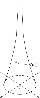
Figure 2: an unbounded domain

By [Ma4, Example 4.3.5/2], if $p>1$,

$${\nu_{p}}(s)\approx\bigg{(}\int_{\Upsilon^{-1}(|\Omega|/2)}^{\Upsilon^{-1}(s)}\zeta(r)^{\frac{1-n}{p-1}}dr\bigg{)}^{1-p}\quad\hbox{for $s\in(0,|\Omega|/2)$.}$$

An application of Theorem 1.1 tells us that there exists a unique solution to problem (1.1) with $f\in L^{q}(\Omega)$ if either $q>1$ and

(5.11) $$\int^{\infty}\bigg{(}\int_{\Upsilon^{-1}(|\Omega|/2)}^{\rho}\zeta(r)^{\frac{1-n}{p-1}}dr\bigg{)}^{\frac{q^{\prime}}{p^{\prime}}}\bigg{(}\int_{\rho}^{\infty}\zeta(r)^{n-1}dr\bigg{)}^{\frac{q^{\prime}}{p}}\zeta(\rho)^{n-1}d\rho<\infty\,,$$

or $q=1$ and

(5.12) $$\int^{\infty}\bigg{(}\int_{\Upsilon^{-1}(|\Omega|/2)}^{\rho}\zeta(r)^{\frac{1-n}{p-1}}dr\bigg{)}^{\frac{1}{p^{\prime}}}\bigg{(}\int_{\rho}^{\infty}\zeta(r)^{n-1}dr\bigg{)}^{-\frac{1}{p^{\prime}}}\zeta(\rho)^{n-1}d\rho<\infty\,.$$

For instance, if $\zeta(\rho)=\frac{1}{(1+\rho)^{\beta}}$, then (5.11) and (5.10) hold if $\beta>\frac{1+q^{\prime}}{n-1}$, whereas (5.12) never holds, whatever $\beta$ is. In the case when $\zeta(\rho)=e^{-\rho^{\alpha}}$ with $\alpha>0$, condition (5.11) holds for every $q\in(1,\infty]$, whereas (5.12) does not hold for any $\alpha$.

Note that, by [Ma4, Example 3.3.3/2],

$$\lambda(s)\approx\big{(}\zeta(\Upsilon^{-1}(s))\big{)}^{n-1}\qquad\hbox{as $s\to 0^{+}$.}$$

Thus, (2.26) holds, and hence Corollary 5.1 leads to the same conclusions.

Example 6 (A domain from [CH])

Let us consider problem (1.1) in the domain $\Omega\subset{\mathbb{R}}^{2}$ displayed in Figure 3 and borrowed from [CH], where it is exhibited as an example of a domain in which the Poincaré inequality fails.

Figure 3: an example from [CH]

In the figure, $L=2^{-k}$ and $l=\delta(2^{-k})$, where $k\in\mathbb{N}$ and $\delta:[0,\infty)\to[0,\infty)$ is any function such that: $\delta(2s)\leq c\delta(s)$ for some $c>0$ and for $s>0$; $\frac{s^{p+1}}{\delta(s)}$ is non-decreasing; $\frac{s^{1+\varepsilon}}{\delta(s)}$ is non-increasing for some $\varepsilon>0$. One can show that, if $1\leq p\leq 2$, then

(5.13) $${\nu_{p}}(s)\approx\delta\big{(}s^{1/2}\big{)}s^{\frac{1-p}{2}}\qquad\quad\hbox{as $s\to 0^{+}$}$$

[CM2]. In particular, by (2.26),

(5.14) $$\lambda(s)\approx\delta\big{(}s^{1/2}\big{)}\qquad\quad\hbox{as $s\to 0^{+}$}.$$

By Theorem 1.1, it is easily verified that there exists a unique solution to problem (1.1) if $f\in L^{q}(\Omega)$ for any $q>1$. When $q=1$, the solution exists and is unique provided that

(5.15) $$\int_{0}\bigg{(}\frac{s}{\delta(s)}\bigg{)}^{1/p}ds<\infty.$$

For instance, (5.15) holds when $\delta(s)=s^{\alpha}$ for some $\alpha\in(1,p+1)$, or when $\delta(s)\approx s^{p+1}\big{(}\log(1/s)\big{)}^{\beta}$ for small $s$, with $\beta>p$.

The use of the isoperimetric function, namely of Corollary 5.1, yield worses results for the domain of this example, for which inequality (5.3) fails. For instance, if $\delta(s)=s^{\alpha}$, the existence and uniqueness of a solution to problem (1.1) cannot be deduced from Corollary 5.1 unless either $\alpha<2$ and $q\geq 1$, or $2\leq\alpha\leq p+1$ and $q>\frac{2}{4-\delta}$.

Example 7 (Nikodým)

The most irregular domain $\Omega\subset{\mathbb{R}}^{2}$ that we consider is depicted in Figure 4. It was introduced by Nikodým in his study of Sobolev embeddings.

Figure 4: Nikodým example

In the figure, $L=2^{-k}$ and $l=\delta(2^{-k})$, where $k\in\mathbb{N}$ and $\delta:[0,\infty)\to(0,\infty)$ is any increasing Lipschitz continuous function such that $\delta(2s)\leq c\delta(s)\leq c^{\prime}s$ for some contants $c,c^{\prime}>0$ and for $s>0$. If $p\geq 1$, one has that

(5.16) $${\nu_{p}}(s)\approx\delta(s)\qquad\quad\hbox{as $s\to 0^{+}$},$$

and

(5.17) $$\lambda(s)\approx\delta(s)\qquad\quad\hbox{as $s\to 0^{+}$}$$

[Ma4, Section 4.5]. By (5.16) and Theorem 1.1 there exists a unique approximable solution to problem (1.1) provided that $f\in L^{q}(\Omega)$ for some $q>1$ and (1.8) is fulfilled, namely

(5.18) $$\int_{0}\bigg{(}\frac{s}{\delta(s)}\bigg{)}^{\frac{q^{\prime}}{p}}ds<\infty\,.$$

On the other hand, condition (1.9) never holds, and hence the case when $f\in L^{1}(\Omega)$ is not admissible in Theorem 1.1 for this domain.

In the special case when

(5.19) $$\delta(s)=s^{\alpha},\qquad\quad\hbox{for $s>0$,}$$

with $\alpha\geq 1$, condition (5.18) is equivalent to

(5.20) $$\alpha<1+\frac{p}{q^{\prime}}\,.$$

Equations (5.17) and (5.16) tell us that (5.3) is not fulfilled for the domain $\Omega$ of this example, and the use of Corollary 5.1 actually requires stronger assumtpions on $\delta(s)$. For instance, when $\delta(s)$ is given by (5.19), one has to demand that $\alpha<2-\frac{1}{q}$. This is a more restrictive condition than (5.20).

References

- [Al] A.Alvino, Formule di maggiorazione e regolarizzazione per soluzioni di equazioni ellittiche del secondo ordine in un caso limite, Atti Accad. Naz. Lincei, Rend. Cl. Sci. Fis. Mat. Natur. 62 (1977), 335–340.
- [AFLT] A.Alvino, V.Ferone, P.-L.Lions & G.Trombetti, Convex symmetrization and applications, Ann. Inst. H. Poincaré Anal. Non Linéaire 14 (1997), 275–293.
- [ALT] A.Alvino, P.-L.Lions & G.Trombetti, Comparison results for elliptic and parabolic equations via Schwarz symmetrization, Ann. Inst. H. Poincaré Anal. Non Linéaire 7 (1990), 37–65.
- [AMT] A.Alvino, S.Matarasso & G.Trombetti, Elliptic boundary value problems: comparison results via symmetrization, Ricerche Mat. 51 (2002), 341–355.
- [AM] A.Alvino & A.Mercaldo, Nonlinear elliptic problems with data: an approach via symmetrization methods, Mediter. J. Math. 5 (2008), 173–185.
- [AFP] L. Ambrosio, N.Fusco & D.Pallara, “Functions of bounded variation and free discontinuity problems”, Clarendon Press, Oxford, 2000.
- [AMST] F.Andreu, J.M.Mazon, S.Segura de Leon & J.Toledo, Quasi-linear elliptic and parabolic equations in with nonlinear boundary conditions, Adv. Math. Sci. Appl. 7 (1997), 183-213.
- [BeGu] A.Ben Cheikh & O.Guibé, Nonlinear and non-coercive elliptic problems with integrable data, Adv. Math. Sci. Appl. 16 (2006), 275–297.
- [BBGGPV] P.Bénilan, L.Boccardo, T.Gallouët, R.Gariepy, M.Pierre & J.L.Vazquez, An -theory of existence and uniqueness of solutions of nonlinear elliptic equations, Ann. Sc. Norm. Sup. Pisa 22 (1995), 241-273.
- [BS] C.Bennett & R.Sharpley, “Interpolation of operators”, Academic Press, Boston, 1988.
- [Be] M.F.Betta, Neumann problems: comparison results, Rend. Accad. Sci. Fis. Nat. Napoli 57 (1990), 41-58.
- [BG1] L.Boccardo & T.Gallouët, Nonlinear elliptic and parabolic equations involving measure data, J. Funct. Anal. 87 (1989), 149–169.
- [BG2] L.Boccardo & T.Gallouët, Nonlinear elliptic equations with right-hand side measures, Comm. Part. Diff. Eq. 17 (1992), 641–655.
- [BuZa] Yu.D.Burago & V.A.Zalgaller, “Geometric inequalities”, Springer-Verlag, Berlin, 1988.
- [CY] S.-Y.A.Chang & P.C.Yang, Conformal deformation of metrics on , J. Diff. Geom. 27 (1988), 259-296.
- [Ch] J.Cheeger, A lower bound for the smallest eigenvalue of the Laplacian, in “Problems in analysis (Papers dedicated to Salomon Bochner, 1969)”, 195–199, Princeton Univ. Press, Princeton, 1970.
- [Ci1] A.Cianchi, On relative isoperimetric inequalities in the plane, Boll. Un. Mat. Ital. 3-B (1989), 289-326.
- [Ci2] A.Cianchi, Elliptic equations on manifolds and isoperimetric inequalities, Proc. Royal Soc. Edinburgh 114A (1990), 213-227.
- [Ci3] A.Cianchi, Moser-Trudinger inequalities without boundary conditions and isoperimetric problems, Indiana Univ. Math. J. 54 (2005), 669-705.
- [CEG] A.Cianchi, D.E.Edmunds & P.Gurka, On weighted Poincaré inequalities, Math. Nachr. 180 (1996), 15-41.
- [CM1] A.Cianchi & V.G.Maz’ya, Neumann problems and isocapacitary inequalites, J. Math. Pures Appl. 89 (2008), 71-105.
- [CM2] A.Cianchi & V.G.Maz’ya, Estimates for solutions to the Schrödinger equation under Neumann boundary conditions, in preparation.
- [CH] R.Courant & D.Hilbert, “Methods of Mathematical Physics”, John Wiley & Sons, New York, 1953.
- [DaA] A.Dall’Aglio, Approximated solutions of equations with data. Application to the -convergence of quasi-linear parabolic equations, Ann. Mat. Pura Appl. 170 (1996), 207–240.
- [Da] G.Dal Maso, Notes on capacity theory, manuscript.
- [DM] G.Dal Maso & A.Malusa, Some properties of reachable solutions of nonlinear elliptic equations with measure data, Ann. Scuola Norm. Sup. Pisa Cl. Sci. 25 (1997), 375–396.
- [DMOP] G.Dal Maso, F.Murat, L.Orsina & A.Prignet, Renormalized solutions of elliptic equations with general measure data, Ann. Sc. Norm. Sup. Pisa Cl. Sci. 28 (1999), 741–808.
- [DLR] A.Decarreau, J.Liang & J.-M.Rakotoson, Trace imbeddings for sets and application to Neumann-Dirichlet problems with measures included in the boundary data, Ann. Fac. Sci. Toulouse 5 (1996), 443–470.
- [De] T.Del Vecchio, Nonlinear elliptic equations with measure data, Potential Anal. 4 (1995), 185–203.
- [DHM] G.Dolzmann, N.Hungerbühler & S. Müller, Uniqueness and maximal regularity for nonlinear elliptic systems of n-Laplace type with measure valued right-hand side, J. Reine Angew. Math. 520 (2000), 1-35.
- [Dr] J.Droniou, Solving convection-diffusion equations with mixed, Neumann and Fourier boundary conditions and measures as data, by a duality method, Adv. Differential Equations 5 (2000), 1341–1396.
- [DV] J.Droniou & J.-L. Vasquez, Noncoercive convection-diffusion elliptic problems with Neumann boundary conditions, Calc. Var. and PDE’s 34 (2009),413–434.
- [EG] L.C.Evans & R.F.Gariepy, “Measure Theorey and Fine Properties of Functions”, CRC PRESS, Boca Raton, 1992.
- [A.Fe] A.Ferone, Symmetrization for degenerate Neumann problems, Rend. Accad. Sci. Fis. Mat. Napoli 60 (1993), 27–46.
- [V.Fe1] V.Ferone, Symmetrization in a Neumann problem, Le Matematiche 41 (1986), 67–78.
- [V.Fe2] V.Ferone, Estimates and regularity for solutions of elliptic equations in a limit case, Boll. Un. Mat. Ital. 8 (1994), 257–270.
- [FS] A.Fiorenza & C.Sbordone, Existence and uniqueness results for solutions of nonlinear equations with right-hand side in , Studia Math. 127 (1998), 223-231.
- [Ga] S.Gallot, Inégalités isopérimétriques et analitiques sur les variétés riemanniennes, Asterisque 163 (1988), 31-91.
- [Go] M.L.Goldman, Sharp estimates for the norms of Hardy-type operators on the cones of quasimonotone functions, Proc. Steklov Inst. Math. 232 (2001), 1-29.
- [GIS] L.Greco, T.Iwaniec & C.Sbordone, Inverting the p-harmonic operator, Manuscripta Math. 92 (1997), 249-258.
- [HK] P.Haiłasz & P.Koskela, Isoperimetric inequalites and imbedding theorems in irregular domains, J. London Math. Soc. 58 (1998), 425-450.
- [HM] H.Heinig & L.Maligranda, Weighted inequalities for monotone and concave functions, Studia Math. 116 (1995), 133–165.
- [Ka1] B.Kawohl, “Rearrangements and convexity of level sets in PDE”, Lecture Notes in Math. 1150, Springer-Verlag, Berlin, 1985.
- [Ke1] S. Kesavan, On a comparison theorem via symmetrisation, Proc. Roy. Soc. Edinburgh Sect. A 119 (1991), 159–167.
- [Ke2] S.Kesavan, “Symmetrization & Applications”, Series in Analysis 3, World Scientific, Hackensack, 2006.
- [KM] T.Kilpeläinen & J.Malý, Sobolev inequalities on sets with irregular boundaries, Z. Anal. Anwendungen 19 (2000), 369–380.
- [La] D.A.Labutin, Embedding of Sobolev spaces on Hölder domains, Proc. Steklov Inst. Math. 227 (1999), 163-172 (Russian); English translation: Trudy Mat. Inst. 227 (1999), 170–179.
- [LL] E.H.Lieb & M.Loss, “Analysis”, American Mathematical Society, Providence, 1997.
- [LM] P.-L.Lions & F.Murat, Sur les solutions renormalisées d’équations elliptiques non linéaires, manuscript.
- [LP] P.-L.Lions & F.Pacella, Isoperimetric inequalities for convex cones, Proc. Amer. Math. Soc. 109 (1990), 477-485.
- [MS1] C.Maderna & S.Salsa, Symmetrization in Neumann problems, Appl. Anal. 9 (1979), 247-256.
- [MS2] C.Maderna & S.Salsa, A priori bounds in non-linear Neumann problems, Boll. Un. Mat. Ital. 16 (1979), 1144-1153.
- [MZ] J.Malý & W. P.Ziemer, “Fine regularity of solutions of elliptic partial differential equations”, American Mathematical Society, Providence, 1997.
- [Ma1] V.G.Maz’ya, Classes of regions and imbedding theorems for function spaces, Dokl. Akad. Nauk. SSSR 133 (1960), 527–530 (Russian); English translation: Soviet Math. Dokl. 1 (1960), 882–885.
- [Ma2] V.G.Maz’ya, Some estimates of solutions of second-order elliptic equations, Dokl. Akad. Nauk. SSSR 137 (1961), 1057–1059 (Russian); English translation: Soviet Math. Dokl. 2 (1961), 413–415.
- [Ma3] V.G.Maz’ya, On weak solutions of the Dirichlet and Neumann problems, Trusdy Moskov. Mat. Obšč. 20 (1969), 137–172 (Russian); English translation: Trans. Moscow Math. Soc. 20 (1969), 135-172.
- [Ma4] V.G.Maz’ya, “Sobolev spaces”, Springer-Verlag, Berlin, 1985.
- [MP] V.G.Maz’ya & S.V.Poborchi, “Differentiable functions on bad domains”, World Scientific, Singapore, 1997.
- [M1] F.Murat, Soluciones renormalizadas de EDP elṕticas no lineales, Preprint 93023, Laboratoire d’Analyse Numérique de l’Université Paris VI (1993).
- [M2] F.Murat, Équations elliptiques non linéaires avec second membre ou mesure, Actes du 26ème Congrés National d’Analyse Numérique, Les Karellis, France (1994), A12-A24.
- [Po] M.M. Porzio, Some results for non-linear elliptic problems with mixed boundary conditions, Ann. Mat. Pura Appl. 184 (2005), 495–531.
- [Pr] A. Prignet, Conditions aux limites non homog nes pour des probl mes elliptiques avec second membre mesure, Ann. Fac. Sci. Toulouse 6 (1997), 297–318.
- [Se] J.Serrin, Pathological solutions of elliptic partial differential equations, Ann. Scuola Norm. Sup. Pisa 18 (1964), 385-387.
- [St] G.Stampacchia, Le problème de Dirichlet pour les équations elliptiques du second ordre à coefficients discontinus, Ann. Inst. Fourier 15 (1965), 189-258.
- [Ta1] G.Talenti, Elliptic equations and rearrangements, Ann. Sc. Norm. Sup. Pisa 3 (1976), 697-718.
- [Ta2] G.Talenti, Nonlinear elliptic equations, rearrangements of functions and Orlicz spaces, Ann. Mat. Pura Appl. 120 (1979), 159-184.
- [Tr] G.Trombetti, Symmetrization methods for partial differential equations, Boll. Un. Mat. Ital. Sez. B 3 (2000), 601-634.
- [Va] J.L.Vazquez, Symmetrization and mass comparison for degenerate nonlinear parabolic and related elliptic equations, Adv. Nonlinear Stud. 5 (2005), 87-131.
- [We] H.F.Weinberger, Symmetrization in uniformly elliptic problems, in Studies in Mathematical Analisis, Stanford Univ. Press, 1962, 424-428.
- [Ze] E.Zeidler, “Nonlinear functional analysis and its applications”, Vol. II/B, Springer-Verlag, New York, 1990.
- [Zi] W.P.Ziemer, “Weakly differentiable functions”, Springer-Verlag, New York, 1989.