Abstract

Light scattering detection in the near field, a rapidly expanding family of scattering techniques, has recently proved to be an appropriate procedure for performing dynamic measurements. Here we report an innovative algorithm, based on the evaluation of the Exposure Time Dependent Spectrum (ETDS), which makes it possible to measure the fast dynamics of a colloidal suspension with the aid of a simple near field scattering apparatus and a CCD camera. Our algorithm consists in acquiring static spectra in the near field at different exposure times, so that the measured decay times are limited only by the exposure time of the camera and not by its frame rate. The experimental set-up is based on a modified microscope, where the light scattered in the near field is collected by a commercial objective, but (unlike in standard microscopes) the light source is a He-Ne laser which increases the instrument sensitivity. The apparatus and the algorithm have been validated by considering model systems of standard spherical nano-particle.

OCIS codes: (290.0290) Scattering; (120.4640) Optical instruments; (180.0180) Microscopy

1 Introduction

During the last few decades, light scattering techniques have demonstrated their ability to provide detailed information about properties of complex fluids. This capability is mainly due to the fact that these methods allow direct measurement of ensemble averages of the spatial and temporal fluctuations of fluid properties, which are precisely the quantities that can be usually calculated by theoretical methods of statistical mechanics, thus making available a simple way to compare experimental results with theory.

More recently, low angle light scattering methods have also became very popular thanks to the advent of pixilated sensors like CCD or CMOS cameras and their continuous technical development. The utilization of such sensors was first proposed by Wong and Wiltzius in 1993 [1] and gave rise to a large number of similar approaches [2, 3]. In these first attempts to utilize a multi-element sensor to gain statistical accuracy (typical sensors have about 1k x 1k pixels, thus providing $10^{6}$ independent measurements at one shot), the sensor was positioned in the Fourier plane of a lens. In this way it was possible to collect the scattered light in the far field, after removing the probe beam by means of a small mirror in the center of the focal plane. Accordingly, we will refer to this family of procedures as Scattering In the Far Field (SIFF) techniques. In order to overcome some of the difficulties experimented with SIFF, an alternative approach was recently proposed, consisting in collecting the light scattered by the sample in the near field, i.e. very close to the sample. We will refer to this second family of techniques as Scattering In the Near Field (SINF). The SINF methods show some advantages with respect to SIFF methods, including the extension of the scattering angle range to arbitrarily small values and the avoidance of stray light problems. Examples of SINF techniques are the shadowgraph [4, 5, 6], the schlieren, the speckle schlieren [7], and the Heterodyne Near Field Scattering (HNFS) [8]. In the present paper, we will consider heterodyne SINF techniques only, in which both the scattered beam and the more intense transmitted beam are conveyed to the sensor. In this case, Fourier analysis of the heterodyne SINF images allows to recover the intensity of the scattered beams from the interference fringes they generate on the nearly uniform transmitted beam.

SINF procedures have also been extended in the time domain in order to perform Dynamic Light Scattering (DLS) measurements [9, 10, 11, 12], offering detailed data of the time correlation functions of the non-equilibrium fluctuations or of the diffusional random walk of colloidal particles. This approach has also been applied to optical microscopy [13], suggesting that, even with incoherent illumination, one can achieve information about sample dynamics.

When using SINF techniques the dynamic data are obtained by acquiring sequences of images at a given frame rate. After the acquisition, the images are Fourier transformed and processed. In the literature two different algorithms have been used to analyze the sequences, namely: (1) calculation of the time-correlation function (or equivalently the time power spectrum) and (2) calculation of the time structure function. In the present paper we introduce and describe a third method, which allows measuring fast dynamics without the need for a fast acquisition.

Approach (1) is fairly similar to the standard procedure used in DLS experiments, where the time-correlation function is obtained by hardware calculation using the data collected by a photo-multiplier tube aligned at a certain angle with the probe beam [14]. For example, this approach has been used on shadowgraph images to investigate the dynamics of spiral defect chaos in high pressure CO₂ [15] and also to analyze the propagating modes that appear in a fluid subjected to a temperature gradient [16].

Method (2) originated from the pioneering proposal by Schulz-DuBois & Rehberg [17] to develop hardware (a so called “structurator”) capable of computing the structure function in place of the standard “correlator”. This technique permits to eliminate the annoying slowly moving drifts that would plague scattering experiments. This was first reported by some of us [9, 10], and was later applied to a broad variety of different experimental methods like X-ray scattering [18], optical microscopy [13] and HNFS [12].

The innovative approach proposed in the present paper is based on the study of the dependence of the (static) image power spectrum on the camera exposure time, hence the name Exposure Time Dependent Spectrum (ETDS). The physical idea behind this technique is that, when increasing the exposure time, the fast dynamics of the images is progressively faded out and what is left are the long time fluctuations only. In practice, increasing the exposure time is equivalent to the application of a sort of low pass filter, averaging the fastest fluctuations and thus depleting the power spectrum. For very long exposure times the fluctuations are completely smeared and we detect the background electronic noise of the CCD camera. Normally, state-of-the-art methods can detect fast dynamics up to the camera frame rate; by contrast, our ETDS method works by acquiring uncorrelated images at a very low frame rate, and the fastest dynamics it can detect is limited only by the shortest exposure time the camera can reach. This methodology intrinsically boosts the performance of any camera, since the shortest gating time is always much shorter than the fastest frame-rate delay. We suggest that the method can yield very impressive results, down to the sub-picosecond scale, by using pulsed lasers or fast-gated cameras or intensifiers. The method has been validated by measuring the time constants of three colloidal particles of different sizes using a HNFS set-up implemented on a microscope.

The rest of the paper is organized as follows: in section 2 the experimental apparatus used to collect scattering images will be described; in section 3 the ETDS will be derived; in section 4 the experimental data for a wide range of wave vectors will be presented; finally, a brief summary of the work will be given.

2 Experimental set up

In Fig. 1 a sketch of the optical set-up is presented. It is based on a modified microscope where the light source is a He-Ne laser (10 mW, NEC) with an output of 0.7 mm diameter TEM00. The beam is used directly, without spatial filtering, because the quality of the unmodified beam has been proved to be enough for our purpose. The laser beam passes through a neutral filter wheel, with transmission range 0.3 - 0.0003. After the filter, the beam is reflected upward by a mirror, and goes through a -5 cm focal-length, negative double-concave lens, in order to increase its diameter. We have checked that the slight divergence of the light impinging on the sample can be neglected. The sample is placed 15 cm after the lens, where the beam diameter is about 2.5 mm wide.

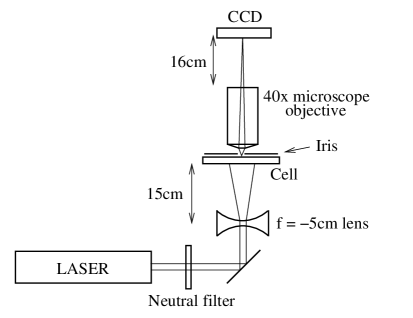
Fig. 1: Scheme of the optical set-up. A plane parallel beam of a He-Ne laser is attenuated by a neutral filter and bend upwards by a mirror. The beam is expanded by means of a negative focal length lens, making it diverge slightly before it enters the sample cell. Scattered light is acquired in the near field together with transmitted light, through a $40\times$ microscope objective, which conjugates a plane close to the sample onto the CCD sensor.

The sample is placed in a glass cell with optical path 1 mm, made of two microscope cover slips, spaced by small glass strips cut from a microscope slide, and glued with silicone rubber. Over the top cover slip, we placed an iris with a 1 mm-diameter aperture, to reduce unwanted reflections. The optical system consists of a plan-achromatic 40x objective (Optika Microscopes, FLUOR), with 0.65 numerical aperture, 160 mm focal distance and 0.17 mm working distance; its focus lies on plane of the iris, about one mm outside the cell. Images are acquired with a CCD camera (Andor Luca), whose sensor is 658 x 496 pixels. The camera’s maximum frame rate is 30 frames per second, with a minimum exposure time of 0.5 ms. The sensor is placed at 160 mm from the microscope objective, so that it collects images directly with a magnification of about 40x. The CCD sensor images an area of $200\times 150\mathrm{\mu m^{2}}$, while the diameter of the illuminated area of the sample is 2.5 mm, thus providing the conditions for near field detection of the light [12]. Each experiment consists of a set of measurements collected at different exposures times. For each measurement a different neutral filter is selected, and the exposure time is adjusted so that the acquired images have an average intensity corresponding to half of the dynamic range. One hundred images are then acquired, at a frame rate of 1 Hz, slowly enough to ensure that all the images are uncorrelated.

3 Image processing

The goal of static scattering measurements is to obtain information about $I\left(\textbf{Q}\right)$, the scattered intensity at transferred wave vector Q, where $\textbf{Q}=\textbf{k}_{s}-\textbf{k}_{i}$, $\textbf{k}_{s}$ is the wave vector of the scattered beam and $\textbf{k}_{i}$ is the wave vector of the incident beam. In conventional static SIFF experiments, the static scattered intensity $I\left(\textbf{Q}\right)$ is obtained by direct measurement, collecting the scattered light by using a photo-multiplier tube or a CCD in the far field at various angles with the impinging beam. By contrast, in a static SINF experiment using a pixilated sensor, we measure instantaneously the image signal $i\left(\textbf{x}\right)$, which is the intensity distribution at point x on a plane close to the sample. After a set of images is acquired, the Image Power Spectrum (IPS) $S_{i}\left(\textbf{q}\right)$ is evaluated, calculating the average of the square modulus of the Fourier transform.

$$S_{i}\left(\textbf{q}\right)=\left<\left|\tilde{i}\left(\textbf{q}\right)\right|^{2}\right>=\left<\left|\mathcal{F}\left[i\left(\textbf{x}\right)\right]\right|^{2}\right>$$ (1)

where $\mathcal{F}\left(\cdot\right)$ is the 2D Fourier transform, q is the 2D spatial wave vector on the image plane, and the mean value $\left<\cdot\right>$ is obtained by averaging over the set of images. Usually, before this Fourier processing, the images are “cleaned” by subtracting the optical background, which is obtained by averaging the images. The IPS $S_{i}(\textbf{q})$ represents the intensity of the Fourier modes, each one corresponding to a diffraction fringe generated by the interference between the transmitted beam and the scattered beam. By calculating the projection of Q on the image plane, it’s easy to show that the transferred wave vector Q is related to the image wave vector q by the following relation:

$$Q\left(q\right)=\sqrt{2}k\sqrt{1-\sqrt{1-\left(\frac{q}{k}\right)^{2}}}$$ (2)

where $k\approx k_{s}\approx k_{i}$ is the light wave vector in the medium. The relation between the IPS $S_{i}\left(\textbf{q}\right)$ and the scattered intensity $I\left[\textbf{Q}\left(\textbf{q}\right)\right]=I\left(\textbf{q}\right)$ is linear, and is actually given [9, 10] by the sum of two terms:

$$S_{i}\left(\textbf{q}\right)=I\left(\textbf{q}\right)\cdot T\left(\textbf{q}\right)+B\left(\textbf{q}\right)$$ (3)

where $T\left(\textbf{q}\right)$ is the instrument transfer function, i.e. a relation between the wave vector and the instrument sensitivity, and $B\left(\textbf{q}\right)$ is the electronic background accounting for noise sources within the grabbing process. The instrument transfer function varies depending on the experimental set-up; it can be simply equal to a constant in the case of HNFS [8, 19] or schlieren [7, 10] thus providing the static scattered intensity with no further complications. Conversely, it has been shown [5, 6, 11] that for a shadowgraph the transfer function exhibits, in some q range, deep oscillations, thus making the retrieval of scattered intensity difficult and providing no information in that vector range. In other cases the instrument transfer function can be completely unpredictable, which makes the static data completely unusable. However, the knowledge of the transfer function is not needed for the dynamic analysis, in which the attention is focused on the time fluctuations of the scattered intensity.

Indeed, the goal of dynamic light scattering is to study the time correlation function of the field $C_{E}\left(\textbf{q},t\right)$. In the case of dynamic SIFF in heterodyne configuration, this quantity is usually directly measured with a correlator; or in the case of homodyne configuration, through Siegert’s relation. Our ETDS-based algorithm for SINF analysis relies on the following argument. As pointed out by Oh et al. [20], when the camera exposure time $\Delta t$ is not negligible, the IPS $S_{i}\left(\textbf{q}\right)$ depends also on $\Delta t$. Hence we will call it ETDS and use the notation $S_{i}\left(\textbf{q},\Delta t\right)$. It is easy to find a relation between the field correlation function $C_{E}\left(\textbf{q},t\right)$ and $S_{i}\left(\textbf{q},\Delta t\right)$ as follows. An image $i\left(\textbf{x},\Delta t\right)$, obtained with an exposure time $\Delta t$, is the results of a time averaging over the instantaneous intensity map $i\left(\textbf{x},t\right)$: $i\left(\textbf{x},\Delta t\right)=\frac{1}{\Delta t}\int_{t_{0}}^{t_{0}+\Delta t}i\left(\textbf{x},t^{\prime}\right)\mathrm{d}t^{\prime}$, where $t_{0}$ is the starting time of the image exposition. The same applies for the Fourier transform: $\tilde{i}\left(\textbf{x},\Delta t\right)=\frac{1}{\Delta t}\int_{t_{0}}^{t_{0}+\Delta t}\tilde{i}\left(\textbf{x},t^{\prime}\right)\mathrm{d}t^{\prime}$. The ETDS is then formally obtained as follows:

$$S_{i}\left(\textbf{q},\Delta t\right)=\left<\left|\tilde{i}\left(\textbf{q},\Delta t\right)\right|^{2}\right>=\frac{1}{\Delta t^{2}}\left<\int_{t_{0}}^{t_{0}+\Delta t}\mathrm{d}t^{\prime}\int_{t_{0}}^{t_{0}+\Delta t}\mathrm{d}t^{\prime\prime}\tilde{i}\left(\textbf{q},t^{\prime}\right)\tilde{i}\left(\textbf{q},t^{\prime\prime}\right)\right>$$

$$=\frac{1}{\Delta t^{2}}\int_{t_{0}}^{t_{0}+\Delta t}\mathrm{d}t^{\prime}\int_{t_{0}}^{t_{0}+\Delta t}\mathrm{d}t^{\prime\prime}C_{i}\left(\textbf{q},t^{\prime}-t^{\prime\prime}\right)$$ (4)

where $C_{i}\left(\textbf{q},t\right)$ is the time correlation function of the Fourier modes of the images. The double integral can be reduced to a simple integral with the following change of variables:

$$\begin{array}[]{l}t^{\prime}=t_{0}+\frac{\Delta t}{2}+\frac{s^{\prime}}{2}+\frac{s^{\prime\prime}}{2}\\ t^{\prime\prime}=t_{0}+\frac{\Delta t}{2}-\frac{s^{\prime}}{2}+\frac{s^{\prime\prime}}{2}\end{array}$$ (5)

Substituting we have:

$$S_{i}\left(\textbf{q},\Delta t\right)=\frac{1}{2\Delta t^{2}}\int_{-\Delta t}^{\Delta t}\mathrm{d}s^{\prime}\int_{-\Delta t+\left|s^{\prime}\right|}^{\Delta t-\left|s^{\prime}\right|}\mathrm{d}s^{\prime\prime}C_{i}\left(\textbf{q},s^{\prime}\right)$$ (6)

The calculation of the integral over $\mathrm{d}s^{\prime\prime}$ gives:

$$S_{i}\left(\textbf{q},\Delta t\right)=\frac{2}{\Delta t^{2}}\int_{0}^{\Delta t}\mathrm{d}s\left(\Delta t-s\right)C_{i}\left(\textbf{q},s\right)$$ (7)

but, in turn, $C_{i}\left(\textbf{q},t\right)$ is related to $C_{E}\left(\textbf{q},t\right)$ and so:

$$S_{i}\left(\textbf{q},\Delta t\right)\propto T\left(\textbf{q}\right)\frac{2}{\Delta t^{2}}\int_{0}^{\Delta t}\mathrm{d}s\left(\Delta t-s\right)C_{E}\left(\textbf{q},s\right)+B\left(\textbf{q}\right)$$ (8)

This is the general relation between $S_{i}\left(\textbf{q},\Delta t\right)$ and the correlation function $C_{E}\left(\textbf{q},t\right)$: the ETDS calculated at a certain exposure time $\Delta t$ is the average of the field correlation function, weighted by a triangular function which vanishes for $s\to\Delta t$. This implies that spectra obtained with different exposure times give different results, and the analysis of this variation as a function of $\Delta t$ brings information about the sample dynamics, or the field correlation function $C_{E}\left(\textbf{q},t\right)$. Now we consider the specific case we studied in our experiments: colloidal particles performing a Brownian motion. In this case the field correlation function is a decreasing exponential:

$$C_{E}\left(\textbf{q},t\right)=I\left(\textbf{q}\right)\exp\left(-\frac{t}{\tau}\right)$$ (9)

The resulting ETDS is:

$$S_{i}\left(\textbf{q},\Delta t\right)\propto I\left(\textbf{q}\right)T\left(\textbf{q}\right)f\left(\frac{\Delta t}{\tau}\right)+B\left(\textbf{q}\right)$$ (10)

where

$$f\left(z\right)=2\frac{\exp\left(-z\right)-1+z}{z^{2}}$$ (11)

The last equation indicates that $S_{i}\left(\textbf{q},\Delta t\right)$ is a decaying function with a characteristic time $\tau$. In general this time constant can be different for different wave vectors Q. For example for diffusing Brownian particles the time constant varies as $\tau\left(Q\right)=1/\left(DQ^{2}\right)$, in which $D$ is the translational diffusion coefficient of the particles in the solvent, as given by the Stokes-Einstein equation.

It’s worth analyzing the limits of the ETDS for very short and very long exposures times:

$$\lim_{\Delta t/\tau\ll 1}S_{i}\left(\textbf{q},\Delta t\right)=I\left(\textbf{q}\right)T\left(\textbf{q}\right)+B\left(\textbf{q}\right)$$ (12)

$$\lim_{\Delta t/\tau\gg 1}S_{i}\left(\textbf{q},\Delta t\right)=B\left(\textbf{q}\right)$$ (13)

For very short exposure times the ETDS approximates the static value of the IPS as given by Eq. (3). For long times the ETDS goes asymptotically to the electronic background of the system.

In summary, by acquiring series of images with many different exposure times and analyzing the ETDS for each single wave vector by using the fitting procedure in Eq. (10) and (11), one obtains a direct and simultaneous measurement of the time constants of the sample for all the measured wave vectors. As a byproduct, one gets also two other terms from the fitting procedure, namely, the product of the static scattered intensity times the instrument transfer function $I\left(\textbf{q}\right)\cdot T\left(\textbf{q}\right)$ and the electronic background of the system.

4 Experimental results

In order to test the validity of the our approach we have performed three experiments with different commercial samples of polystyrene nano-particles of 80 nm, 150 nm and 400 nm diameter (Polyscience Inc.). The particles are well mono-dispersed and the declared size corresponds to the measured size within 5% (81$\pm$4 nm, 149$\pm$5 nm, 402$\pm$12 nm respectively) as checked by a traditional DLS apparatus (Brookhaven Instruments, ZetaPlus). The two smallest samples have been dispersed in water at a concentration of 0.1% w/w, whereas the largest ones have been prepared in water at a concentration of about 0.001% w/w. All the samples gave a sufficiently high scattering signal and for each sample, various sequences of 100 images were acquired at 7 different exposure times $\Delta t$ of about 0.5 ms, 1.5 ms, 5.5 ms, 18 ms, 55 ms, 180 ms, and 550 ms. For each sequence, the ETDS was calculated. The optical background due to stray light contributions was removed from each image by subtracting the image average obtained over the set of images for each exposure time. In Fig. 2 we show the images obtained with the 80 nm particles at four different exposure times. As it is apparent from the figures, as the exposure time increases the appearance of the images changes, and the short scale inhomogeneities are progressively smeared.

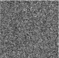
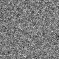
a)	b)
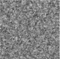
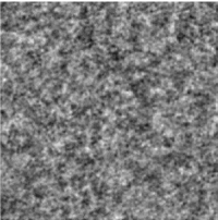
c)	d)

Fig. 2: Acquired images of nano-particles of 80 nm diameter at four different exposure times $\Delta t$ (a) 18 ms, b) 55 ms, c) 180 ms, d) 550 ms). The image size corresponds to $75\times 75\mu m^{2}$ in real space.

In Fig. 3 the $S_{i}\left(\textbf{q},\Delta t\right)$ spectrum for 80 nm particles is shown at different exposure times. This data show clearly that the spectra decrease as the exposure time is increased. For the longest exposure time the averaging of the fluctuations reduces the scattering signal towards the electronic background level.

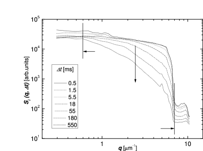
Fig. 3: Exposure Time Dependent Spectra $S_{i}\left(\textbf{q},\Delta t\right)$ measured as a function of the scattering vector q, at different exposure times $\Delta t$ for particles of 80 nm diameter. The central arrow indicates the increase of the exposure time, while the vertical lines indicate the lower and upper boundaries of the q range over which the fitting procedure has been performed.

In Fig. 4 the $S_{i}\left(\textbf{q},\Delta t\right)$ spectra are represented as a function of the exposure time at 4 different wave vectors. It’s possible to observe the different decay times and the different amplitudes of the electronic background. Fitting curves obtained by using equations 4 and 5 are displayed, too. The fitting is carried out with three free parameters, namely, the time constant $\tau\left(\textbf{q}\right)$, the product of the static scattered intensity times the instrument transfer function $I\left(\textbf{q}\right)\cdot T\left(\textbf{q}\right)$, and the electronic background of the system $B\left(\textbf{q}\right)$. The agreement between data points and the corresponding fitting curves is very good. It’s worth pointing out that, even if this fitting is made with such a limited number of data-points, each point is the output of a statistical analysis of 100 images and several statistically independent samples. is the number of independent samples is about $n\approx\pi q/q_{min}$, where $q_{min}$ is the minimum wave vector. This means that in the wave vector range of interest the number of statistical samples for each point in Fig. 4 varies from 3,000 to 30,000.

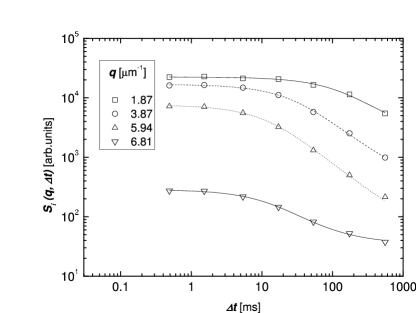
Fig. 4: Exposure time dependent spectra $S_{i}\left(\textbf{q},\Delta t\right)$ measured as a function of the exposure times $\Delta t$, at four different wave vectors $q$, for particles of 80 nm diameter. Lines correspond to fitting curves determined by Eq. 10 and 11 see the main text for details.

In Fig. 5 the time constants obtained by the proposed fitting procedure are plotted for the different samples as a function of the wave vector. Lines correspond to fitting of $\tau$ values according to the formula $\tau\left(Q\right)=1/\left(DQ^{2}\right)$. This fitting procedure has only $D$ as an adjustable parameter; the particle diameter can be recovered from the Stokes-Einstein equation. Obtained diameters are 81$\pm$2 nm, 138$\pm$7 nm and 427$\pm$12 nm, in very good agreement with the sizes measured by standard DLS.

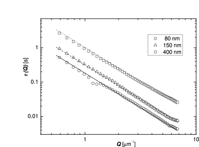
Fig. 5: Time constant $\tau$ measured as a function of the wave vector $q$, for 3 different particle sizes. Straight lines in the log-log plot correspond to fitting curves with the power law $\tau\left(Q\right)=1/\left(DQ^{2}\right)$.

5 Conclusions

In the present work we have presented results from a dynamic near field scattering experiment, performed on colloidal particles by means of a simple set-up, consisting of a suitable modified optical microscope and a laser beam as illuminating light. A new statistical algorithm is presented that allows us to measure the characteristic time constants of the colloidal system. The statistical procedure enables the camera to detect characteristic times much shorter than the camera delay times. Indeed, the only limitation is associated with the minimum exposure time of the camera and not by its delay time. This result opens the way to the investigation of ultra-fast dynamics such as molecular motions, capillary waves, nano-particles diffusion, and virus or biological macromolecules mobility. Until now these phenomena required sophisticated equipment, whereas the proposed method uses a simple modified microscope and a standard camera.