High-statistics study of ${\boldmath\eta\pi^{0}}$ production in two-photon collisions

Abstract

The differential cross section for the process $\gamma\gamma\to\eta\pi^{0}$ has been measured in the kinematic range $0.84~{}{\rm GeV}<W<4.0~{}{\rm GeV}$, $|\cos\theta^{*}|<0.8$, where $W$ and $\theta^{*}$ are the energy and $\pi^{0}$ (or $\eta$) scattering angle, respectively, in the $\gamma\gamma$ center-of-mass system. The results are based on a 223 fb^-1 data sample collected with the Belle detector at the KEKB $e^{+}e^{-}$ collider. Clear peaks due to the $a_{0}(980)$ and $a_{2}(1320)$ are visible. The differential cross sections are fitted in the energy region $0.9~{}{\rm GeV}<W<1.46~{}{\rm GeV}$ to obtain the parameters of the $a_{0}(980)$. Its mass, width and $\Gamma_{\gamma\gamma}{\cal B}(\eta\pi^{0})$ are measured to be $982.3~{}^{+0.6}_{-0.7}~{}^{+3.1}_{-4.7}~{}{\rm MeV}/c^{2}$, $75.6\pm 1.6~{}^{+17.4}_{-10.0}~{}{\rm MeV}$ and $128~{}^{+3}_{-2}~{}^{+502}_{-43}~{}{\rm eV}$, respectively. The energy and angular dependences above 3.1 GeV are compared with those measured in the $\pi^{0}\pi^{0}$ channel. The integrated cross section over $|\cos\theta^{*}|<0.8$ has a $W^{-n}$ dependence with $n=10.5\pm 1.2\pm 0.5$, which is slightly larger than that for $\pi^{0}\pi^{0}$. The differential cross sections show a $\sin^{-4}\theta^{*}$ dependence similar to $\gamma\gamma\to\pi^{0}\pi^{0}$. The measured cross section ratio, $\sigma(\eta\pi^{0})/\sigma(\pi^{0}\pi^{0})=0.48\pm 0.05\pm 0.04$, is consistent with a QCD-based prediction.

The Belle Collaboration

I Introduction

Measurements of exclusive hadronic final states in two-photon collisions provide valuable information concerning physics of light and heavy-quark resonances, perturbative and non-perturbative QCD and hadron-production mechanisms. So far, we have measured the production cross sections for charged-pion pairs mori1 ; mori2 ; nkzw , charged and neutral-kaon pairs nkzw ; kabe ; wtchen , and proton-antiproton pairs kuo . We have also analyzed $D$-meson-pair production and observe a new charmonium state identified as the $\chi_{c2}(2P)$ uehara . In addition, we have measured the $\pi^{0}\pi^{0}$ final state pi0pi0 ; pi0pi02 . The statistics of these measurements is two to three orders of magnitude higher than pre-$B$-factory measurements past_exp , opening a new era in studies of two-photon physics.

In this paper, we report measurements of the differential cross sections, $d\sigma/d|\cos\theta^{*}|$, for the process $\gamma\gamma\to\eta\pi^{0}$ in a wide two-photon center-of-mass (c.m.) energy ($W$) range from 0.84 GeV to 4.0 GeV and in the c.m. angular range, $|\cos\theta^{*}|\leq 0.8$. We use only the $\eta\to\gamma\gamma$ and $\pi^{0}\to\gamma\gamma$ decay modes in this analysis. The decay mode $\eta\to\pi^{+}\pi^{-}\pi^{0}$ is not used because of a much lower product of efficiency and branching fraction.

Previously, it was reported that this reaction is dominated by resonance production cbep . We can restrict the $I^{G}J^{PC}$ quantum numbers of the meson produced by two photons to be $1^{-}$(even)⁺⁺, that is, those of $a_{J={\rm even}}$ mesons. A long-standing puzzle in QCD is the existence and structure of low mass scalar mesons. In the $I=0$ sector, we recently observed a peak for the $f_{0}(980)$ in both the $\gamma\gamma\to\pi^{+}\pi^{-}$ and $\gamma\gamma\to\pi^{0}\pi^{0}$ channels mori1 ; pi0pi0 . The two-photon width of the $f_{0}(980)$ is measured to be $200-300$ eV, supporting its $q^{2}\bar{q^{2}}$ nature achasov . Our analysis also suggests the existence of another $f_{0}$ meson in the 1.2-1.5 GeV region that couples with two photons pi0pi0 . In the $I=1$ sector, the $a_{0}(980)$ and $a_{2}(1320)$ have been observed previously with a rather low statistical significance cbep ; jade . The parameters for the $a_{0}(980)$, in particular its two-photon width are of great interest because of its connection to the nature of low mass scalar mesons. Moreover, other scalar or tensor $a_{J}$ mesons can be searched for in the higher mass region above the prominent peak from the $a_{2}(1320)$.

If there were an $I=1$ “hidden-charm” (that is, charmonium-like) meson, it could be a very strong candidate for an exotic state, because charmonia have $I=0$ and isospin is conserved in their hadronic decays. However, recently, some new particles that are not pure $I=0$, such as the $X(3872)$ x3872 and $Z(4430)$ z4430 , have been reported.

At higher energies ($W>2.4$ GeV), we can invoke a quark model. In leading-order calculations, the ratio of the $\eta\pi^{0}$ cross section to that of $\pi^{0}\pi^{0}$ is predicted within uncertainties due to the different form factors for the $\pi^{0}$ and $\eta$. Analyses of energy and angular distributions of these cross sections are essential to determine properties of the observed resonances and to test the validity of QCD based models bl ; handbag .

This paper is organized as follows. In Sec. II, the experimental apparatus used and the event selection are described. Section III explains background subtraction and derivation of the differential cross sections. In Sec. IV the resonance parameters of the $a_{0}(980)$ are derived by parameterizing partial wave amplitudes with resonances and smooth non-resonant background amplitudes and fitting differential cross sections. Section V describes analyses at higher energy. The topics included there are the angular dependence of differential cross sections, the $W$ dependence of the total cross section, and the ratio of cross sections for $\eta\pi^{0}$ to $\pi^{0}\pi^{0}$ production. Finally, Section VI summarizes the results and presents the conclusion of this paper.

II Experimental apparatus and event selection

Events consisting only of neutral final states are extracted from the data collected in the Belle experiment. In this section, the Belle detector and event selection procedure are described.

II.1 Experimental apparatus

A comprehensive description of the Belle detector is given elsewhere belle . We mention here only those detector components that are essential for the present measurement. Charged tracks are reconstructed from hit information in the silicon vertex detector and the central drift chamber (CDC) located in a uniform 1.5 T solenoidal magnetic field. The detector solenoid is oriented along the $z$ axis, which points in the direction opposite to that of the positron beam. Photon detection and energy measurements are performed with a CsI(Tl) electromagnetic calorimeter (ECL).

For this all-neutral final state, we require that there be no reconstructed tracks coming from the vicinity of the nominal collision point. Therefore, the CDC is used for vetoing events with charged track(s). The photons from decays of the neutral pion and the $\eta$ meson are detected and their momentum vectors are measured by the ECL. The ECL is also used to trigger signal events. Two kinds of the ECL trigger are used to select events of interest: the ECL total energy deposit in the triggerable acceptance region (see the next subsection) is greater than 1.15 GeV (the “HiE” trigger), or the number of ECL clusters counted according to the energy threshold at 110 MeV for segments of the ECL is four or larger (the “Clst4” trigger). The above energy thresholds are determined by studying the correlations between the two triggers in the experimental data. No software filtering is applied for triggering events by either or both of the two ECL triggers.

II.2 Experimental data and data filtering

We use a 223 fb^-1 data sample from the Belle experiment at the KEKB asymmetric-energy $e^{+}e^{-}$ collider kekb . The data were recorded at several $e^{+}e^{-}$ c.m. energies summarized in Table 1. The difference of the luminosity functions (two-photon flux per $e^{+}e^{-}$-beam luminosity) in the measured $W$ regions due to the difference of the beam energies is small (maximum $\pm$ 4%). We combine the results from the different beam energies. The effect on the cross section is less than 0.5%.

Table 1: Data sample: luminosities and energies

$e^{+}e^{-}$ c.m. energy	Luminosity	Runs
(GeV)	(fb-1)
10.58	179	$\Upsilon(4S)$
10.52	19	continuum
10.36	2.9	$\Upsilon(3S)$
10.30	0.3	continuum
10.86	21.7	$\Upsilon(5S)$
Total	223

The analysis is carried out in the “zero-tag” mode, where neither the recoil electron nor positron are detected. We restrict the virtuality of the incident photons to be small by imposing a strict requirement on the transverse-momentum balance with respect to the beam axis for the final-state hadronic system.

The filtered data sample (“Neutral Skim”) used for this analysis is the same as the one used for $\pi^{0}\pi^{0}$ studies pi0pi0 ; pi0pi02 . The important criteria in this filtering are: no good tracks; two or more photons or one or more neutral pions that satisfy a specified energy or transverse-momentum criterion. Performance of the ECL triggers is studied in detail using the $\pi^{0}\pi^{0}$ events  pi0pi0 .

II.3 Event selection

From the Neutral Skim event sample, we select $\gamma\gamma\to\eta\pi^{0}$ with the following conditions:

• the total energy deposit in ECL is smaller than 5.7 GeV;

• there are exactly four photons in the ECL each having energy larger than 100 MeV;

• the ECL energy sum within the triggerable region is larger than 1.25 GeV, or, all the four photons are within the triggerable region, i.e. in the polar-angle range, $-0.6255<\cos\theta<+0.9563$, in the laboratory frame;

• a combination of two photons is reconstructed as a neutral pion that satisfies the following conditions on invariant mass, $|M(\gamma\gamma)-0.1350~{}{\rm GeV}/c^{2}|<0.0200~{}{\rm GeV}/c^{2}$, transverse momentum $p_{t}(\pi^{0})>0.15~{}{\rm GeV}/c$ and goodness of the mass-constrained fit $\chi^{2}<9$;

• the combination of the remaining two photons has an invariant mass consistent with $\eta\to\gamma\gamma$, $0.51~{}{\rm GeV}/c^{2}<M(\gamma\gamma)<0.57~{}{\rm GeV}/c^{2}$. There are three combinations of photon pairs that can be constructed from the four photons, and all the combinations are tried and any of them satisfying the above criteria are retained. We scale the energy of the two photons in (5) with a factor that is the ratio of the nominal $\eta$ mass to the reconstructed mass. This is equivalent to an approximate 1-C mass constraint fit where the relative energy resolution ($\Delta E/E$) is independent of $E$ and the resolution in the angle measurement is much better than that of the energy. The present case is close to this. After scaling the $\eta$’s four-momentum, we calculate the invariant mass ($W$) and the transverse momentum ($|\Sigma{\mbox{{\boldmath$p$}}}_{t}^{*}|$) in the $e^{+}e^{-}$ c.m. frame for the $\eta\pi^{0}$ system.

• The transverse momentum is is required to be less than $0.05~{}{\rm GeV}/c$.

We define the c.m. scattering angle, $\theta^{*}$, as the scattering angle of the $\pi^{0}$ (or equivalently, of the $\eta$ ) in the $\gamma\gamma$ c.m. frame, for each event. We use an approximation that the $e^{+}e^{-}$ axis is the reference for this polar angle as (since we do not know the exact $\gamma\gamma$ axis in the zero-tag condition).

Signal and background events for $e^{+}e^{-}\to e^{+}e^{-}\eta\pi^{0}$ are generated using the TREPS code treps . All Monte Carlo (MC) events are put through the trigger and detector simulators and the event selection program. We find that up to 2% of events in the region below $W<1.05~{}{\rm GeV}$ have two entries per event because of the multiple combinations satisfying criteria (4), (5) and (6). The two entries per event have similar $W$ and $|\Sigma{\mbox{{\boldmath$p$}}}_{t}^{*}|$, but different $|\cos\theta^{*}|$ values. The fraction with double entries is small and is in principle compensated by the normalization using the efficiency determined by the MC sample. We find a similar fraction of multiple entries in the signal-MC data.

A total of $2.82\times 10^{5}$ events are selected from $3.53\times 10^{8}$ events of the Neutral Skim sample. The lego plots of two-dimensional distributions of the selected events (after requiring $|\Sigma{\mbox{{\boldmath$p$}}}_{t}^{*}|<50$ MeV/$c$) are shown in Fig. 1. The projected $W$ distribution integrated over $|\cos\theta^{*}|<0.8$ is shown in Fig. 2. We find at least three resonant structures: near 0.98 GeV ($a_{0}(980)$), 1.32 GeV ($a_{2}(1320)$) and 1.7 GeV (probably the $a_{2}(1700)$).

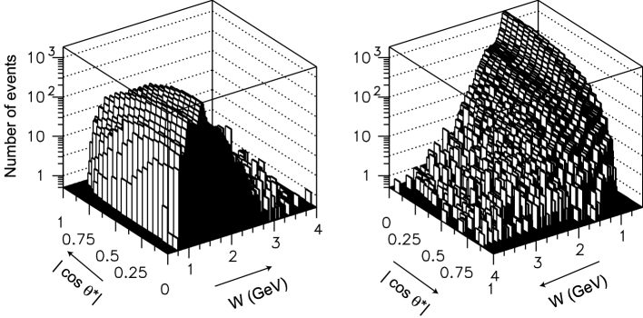
Figure 1: Two-dimensional $W$ and $|\cos\theta^{*}|$ distribution of the $\eta\pi^{0}$ candidates in data. The same distribution is viewed from two different directions.

Figure 2: $W$ distribution for $\eta\pi^{0}$ candidate events integrated over $|\cos\theta^{*}|<0.8$. The solid curve is the $p_{t}$-unbalanced background that are experimentally determined. The dashed curve includes an additional contribution from the $\eta^{\prime}\to\eta\pi^{0}\pi^{0}$ background.

III Deriving differential cross sections

In this section, we present the procedure to derive differential cross sections. First, the nature and origin of backgrounds and the method for their subtraction are described. Unfolding is then applied, efficiencies are determined, differential cross sections are derived and their systematic errors are estimated.

III.1 Background subtraction

In the entire energy range the background is primarily from photons originated from spent electrons as identified by unbalanced $p_{t}$. At low energy there is additional background from the $\eta^{\prime}$ decaying into $\eta\pi^{0}\pi^{0}$.

III.1.1 Background from $\eta^{\prime}\to\eta\pi^{0}\pi^{0}$

A scatter plot of $p_{t}$ balance vs. invariant mass for the candidate events, Fig. 3(a), shows a concentration of events in the $p_{t}$-unbalanced region in the vicinity of 0.82 GeV. This energy is close to the mass difference between the $\eta^{\prime}$ and $\pi^{0}$, and this structure is due to the background from $\eta^{\prime}\to\eta\pi^{0}\pi^{0}$ where two photons from one $\pi^{0}$ are undetected. Since the background is larger than the signal in the $\eta^{\prime}$ mass region, we cannot measure the cross section below $W<0.84~{}{\rm GeV}$. Kinematically, for $\eta^{\prime}$ decays the invariant mass of the detected $\eta\pi^{0}$ system cannot be greater than $0.823~{}{\rm GeV}/c^{2}$. However, there is a rather long tail on the higher side up to $W\sim 0.88~{}{\rm GeV}$. This background is due to a fake pion reconstructed from a photon with another photon from a $\pi^{0}$ or a noise cluster. Figure 3(b) shows that $\eta$ mesons are relatively cleanly reconstructed.

We subtract the background from primary $\eta^{\prime}$s in two-photon collisions using MC. The normalization of the $\eta^{\prime}\to\eta\pi^{0}\pi^{0}$ background is determined using the experimental data in the control region, $0.80~{}{\rm GeV}<W<0.84~{}{\rm GeV}$ integrated over all angles and the transverse-momentum range, $|\Sigma{\mbox{{\boldmath$p$}}}_{t}^{*}|<0.15~{}{\rm GeV}/c$ (Fig. 4(a)). We assume that the signal yield is negligibly small in this $W$ range. The $p_{t}$ distribution is decomposed into the $\eta^{\prime}$ background peaking near $0.05~{}{\rm GeV}/c$ and the other $p_{t}$-unbalanced component by performing a fit, where we use the signal and background functional shapes described in the next subsection for the $\eta^{\prime}$ and the latter background, respectively. The shape parameters of the $\eta^{\prime}$ component are fixed to those obtained from the fit to the corresponding MC data.

From the product of the two-photon decay width and the branching fraction of the $\eta^{\prime}$, $\Gamma_{\gamma\gamma}(\eta^{\prime}){\cal B}(\eta^{\prime}\to\eta\pi^{0}\pi^{0})$, we can estimate the absolute size of the background yield from this source. The ratio of the observed background to the MC expectation is $0.91\pm 0.02(stat.)\pm 0.09(syst.)\pm 0.06(\Gamma_{\gamma\gamma}{\cal B})$, where the first two errors are experimental, and the last error is from the uncertainty of the known $\eta^{\prime}$ properties. This factor is consistent with unity.

Using the normalization thus determined and the MC events, the background yields from this source in each angular bin in the range $0.84~{}{\rm GeV}<W<0.90~{}{\rm GeV}$ are determined. This background component is incorporated in the fit described in the next subsection with the yield and shape fixed. We neglect the $\eta^{\prime}$ background in the $W$ region above 0.90 GeV.

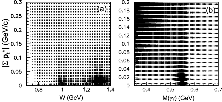
Figure 3: (a)Two-dimensional ($W$, $|\sum{\mbox{{\boldmath$p$}}}_{t}^{*}|$) distribution of the $\eta\pi^{0}$ candidate events in the relatively low-$W$ region. (b)Two-dimensional distribution of the invariant mass of the two detected photons near the $\eta$ mass and the $p_{t}$-balance of events calculated from the mass of four photons (before applying the mass constraints) for events with $M(\eta\pi^{0})<1.0~{}{\rm GeV}/c^{2}$.

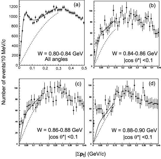
Figure 4: (a): The $p_{t}$ distribution of the $\eta\pi^{0}$ candidates at $W=0.80$-0.84 GeV integrated over $|\cos\theta^{*}|<0.8$. The peak near $0.05~{}{\rm GeV}/c$ is attributed to the background from $\eta^{\prime}\to\eta\pi^{0}\pi^{0}$ and the normalization is determined by a fit to MC events of this process. The dashed curve shows the experimentally determined background from the $p_{t}$-unbalanced background component and the solid curve is the sum of the two background components. (b), (c) and (d): The $p_{t}$ distribution of the $\eta\pi^{0}$ candidate events in the shown kinematical regions. Estimated background yields of the two components are shown by the curves (explained in the caption for (a)). The excess over the solid curve near $|\sum{\mbox{{\boldmath$p$}}}_{t}^{*}|=0$ corresponds to the signal process.

III.1.2 Subtraction of backgrounds

In the $W$ region below 2.0 GeV, the $p_{t}$-unbalanced component is non-negligible and is subtracted by fitting the $p_{t}$ distributions. The fitting function is a sum of the signal and background components. The $\eta^{\prime}$ background estimated in the previous subsection is incorporated in the fit with a fixed shape and size for $W<0.90$ GeV (Figs. 4(b-d)).

The signal component follows an empirical parameterization from signal MC:

$$y=\frac{Ax}{x^{2.1}+B+Cx}\;,$$ (1)

($x$ is $|\sum{\mbox{{\boldmath$p$}}}_{t}^{*}|$, $A$, $B$ and $C$ are fitting parameters), where the distribution has a linear shape near $x=0$ and decreases as $\sim x^{-1.1}$ at large $x$. Here $B$ is an important parameter that determines the peak position; the peak is at $x=B^{\frac{1}{2.1}}/1.1$. The background is parameterized by a linear function vanishing at $x=0$ in $x<50$ MeV/$c$ and a second-order polynomial for $x>50$ MeV/$c$ connected smoothly (up to the first derivative) at $x=50$ MeV/$c$. Fits are applied for $|\Sigma{\mbox{{\boldmath$p$}}}_{t}^{*}|<200$ MeV/$c$ in each bin of $W<2.0$ GeV and $|\cos\theta^{*}|<0.8$ with the bin widths of 0.04 GeV and 0.1 for the two directions, respectively.

The background yields found from the fits are fitted to a smooth two-dimensional function of ($W$, $|\cos\theta^{*}|$), in order to minimize the statistical fluctuations from the MC simulation. In Fig. 2, the curves corresponding to the background thus determined are shown, as well as the fixed background from $\eta^{\prime}$ decays.

The backgrounds are subtracted from the experimental yield distribution. The $\eta^{\prime}$ background estimated in the previous subsection is also subtracted at $W<0.90~{}{\rm GeV}$. The error arising from this background subtraction is taken into account as a systematic error (see the subsection E).

To confirm the validity of the background subtraction method, we examine the $W$ dependence of the yield ratio $R$ defined as:

$$R=\frac{Y(0.15~{}{\rm GeV}/c<|\sum\mbox{{\boldmath$p$}}_{t}^{*}|<0.20~{}{\rm GeV}/c)}{Y(|\sum\mbox{{\boldmath$p$}}_{t}^{*}|<0.05~{}{\rm GeV}/c)}\;,$$ (2)

where $Y$ is the yield in the specified region. We observe that structures have similar features as those seen in the estimated $p_{t}$-unbalanced background (Fig. 5). There is a peaking structure in the background around $W=1.5$ GeV, and a small enhancement just above 2.0 GeV. No significant structures are seen from 2.5 GeV up to $\sim 3.3$ GeV.

We observe a significant increase of $R$ above 3.3 GeV. Such an increase is not reproduced by the MC simulation, where only a slow increase of $R$ ($R=0.15$ at 2.0 GeV and $R=0.25$ at 4.0 GeV) is expected. The excess of $R$, $\Delta R$, is the contribution from multibody background processes. We apply a background subtraction with the background contamination level estimated to be $\Delta R/6$. This factor is obtained by assuming a quasi-linear $|\sum\mbox{{\boldmath$p$}}_{t}^{*}|$ dependence of the background and extracting its leakage into the signal region ($|\sum\mbox{{\boldmath$p$}}_{t}^{*}|<0.05~{}{\rm GeV}/c$), which is approximately 1/6 of the yield in the $0.15~{}{\rm GeV}/c<|\sum\mbox{{\boldmath$p$}}_{t}^{*}|<0.20~{}{\rm GeV}/c$ region. We take a half of the correction (i.e. $\Delta R/12$) as the systematic error from this source if this systematic is larger than the 3% uncertainty nominally applied for the whole region above 2.0 GeV (see the section on systematic errors). The actual sizes of the correction used (i.e. $\Delta R/6$) in $W$ bins are 3.8% (3.35 GeV), 8.5% (3.65 GeV), and 13.0% (3.95 GeV), respectively. These corrections are much smaller than the statistical errors in these $W$ bins.

We find that the background in the $\eta$ mass sideband is negligibly small after the subtraction of these backgrounds; there are no $p_{t}$-balanced backgrounds in the $\eta$ mass sideband of the $p_{t}$-balance distribution shown in Fig. 3(b). Therefore, we do not perform background subtraction for the non-$\eta$ component.

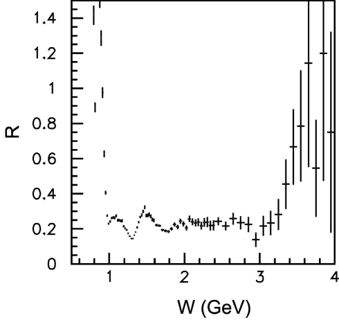
Figure 5: Energy dependence of the ratio of the yield in the $p_{t}$-unbalanced region to that in the balanced region (see text for the exact definition), which indicates the level of background contamination.

III.2 Unfolding the $W$ distributions

We unfold the experimental yields in the $W$ distributions to correct for the finite invariant-mass resolution in the measurement. The smearing function is an asymmetric Gaussian function, which is determined by the signal MC with a further empirical correction. The standard deviations of the function are assumed to follow $1.3\times(1.4-0.3/W^{2})$% ($W$ is in GeV, and the resolution varies by 1.3%-1.8% depending on $W$) on the lower side of the peak and $0.77\times(1.4-0.3/W^{2})$% (varies by 0.8%-1.1%) on the higher side. The resolution is slightly better than that in the $\pi^{0}\pi^{0}$ case in the low $W$ region, because of the large opening angle of the two photons from $\eta$ decay.

The unfolding procedure is applied for 0.9 GeV $<W<$ 1.6 GeV with a bin width of 0.02 GeV, and for 1.6 GeV $<W<$ 2.4 GeV with a bin width of 0.04 GeV. The unfolding is done independently in each angular bin, whose width is $\Delta|\cos\theta^{*}|=0.05$ for $W<1.6$ GeV and $\Delta|\cos\theta^{*}|=0.1$ for $W>1.6$ GeV. Figure 6 shows the yield distributions before and after the unfolding in the smallest $|\cos\theta^{*}|$ bins. At higher energies, no unfolding is applied since the experimental yield is still insufficient.

Figure 6: The yield distributions before (triangles) and after (diamonds) the unfolding in the smallest $|\cos\theta^{*}|$ bins, (a) $|\cos\theta^{*}|<0.05$ and (b) $|\cos\theta^{*}|<0.1$.

III.3 Determination of the efficiency

The signal MC events for $e^{+}e^{-}\to e^{+}e^{-}\eta\pi^{0}$ are generated using the TREPS code treps for the efficiency calculation at 36 fixed $W$ points between 0.75 and 4.2 GeV and isotropically in $|\cos\theta^{*}|$. The angular distribution at the generator level does not play a role in the efficiency determination, because we calculate the efficiencies separately in each $|\cos\theta^{*}|$ bin with a width of 0.05. The $Q^{2}_{\rm max}$ parameter that gives a maximum virtuality of the incident photons is set to 1.0 GeV², and the form factor for the cross sections for the virtual photon collisions, $\sigma_{\gamma\gamma}(0,Q^{2})=\sigma_{\gamma\gamma}(0,0)/(1+Q^{2}/W^{2})^{2}$ is used. This form factor does not play any essential role in the present analysis, since our stringent $p_{t}$-balance cut ($|\sum\mbox{{\boldmath$p$}}_{t}^{*}|<0.05~{}{\rm GeV}/c$) requires $Q^{2}/W^{2}$ for the selected events to be much smaller than 1. A sample of 400,000 events is generated at each $W$ point and is subjected to the detector and trigger simulations. The obtained efficiencies are fitted to a two-dimensional function of ($W$, $|\cos\theta^{*}|$) with an empirical functional form.

We embed background hit patterns from random trigger data into MC events. We find that different samples of background hits give small variations in the selection efficiency determination. A $W$-dependent error in the efficiency, 2-4%, arises from the uncertainty in this effect. Figure 7 shows the two-dimensional dependence of the efficiency on ( $W$, $|\cos\theta^{*}|$) after the fit for smoothing.

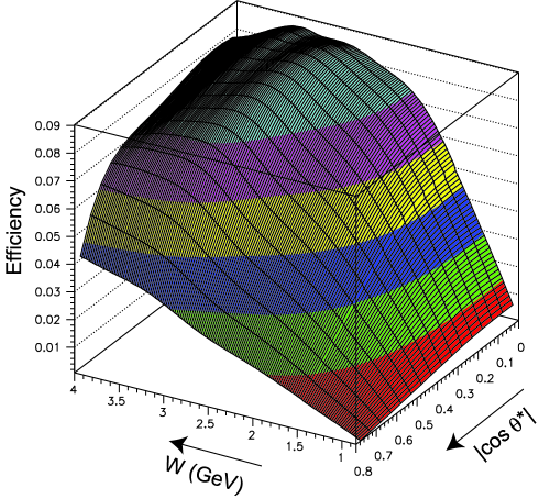
Figure 7: Two-dimensional dependence of the efficiency on ($W$, $|\cos\theta^{*}|$).

III.4 Derivation of differential cross sections

The differential cross section for each ($W$, $|\cos\theta^{*}|$) point is given by:

$$\frac{d\sigma}{d|\cos\theta^{*}|}=\frac{\Delta Y-\Delta B}{\Delta W\Delta|\cos\theta^{*}|\int{\cal L}dtL_{\gamma\gamma}(W)\eta}\;,$$ (3)

where $\Delta Y$ and $\Delta B$ are the signal yield and the estimated $p_{t}$-unbalanced background in the bin, $\Delta W$ and $\Delta|\cos\theta^{*}|$ are the bin widths, $\int{\cal L}dt$ and $L_{\gamma\gamma}(W)$ are the integrated luminosity and two-photon luminosity function calculated by TREPS treps , respectively, and $\eta$ is the efficiency including the correction described in the previous section. The bin sizes for $W$ and $\Delta|\cos\theta^{*}|$ are summarized in Table 2.

Table 2: Bin sizes

$W$ range	$\Delta W$	$\Delta|\cos\theta^{*}|$
(GeV)	(GeV)
0.84 – 1.6	0.02	0.05
1.6 – 2.4	0.04	0.10
2.4 – 4.0	0.10	0.10

Figure 8 shows the angular dependence of the differential cross sections for some selected $W$ regions. Figures 9 show the cross section integrated over $|\cos\theta^{*}|<0.8$ on logarithmic and linear scales for partial $W$ regions. The data points are in good agreement with those of Crystal Ball cbep .

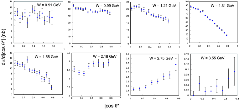
Figure 8: Angular dependence of the differential cross sections for eight selected $W$ bins indicated. The bin sizes are summarized in Table 2.

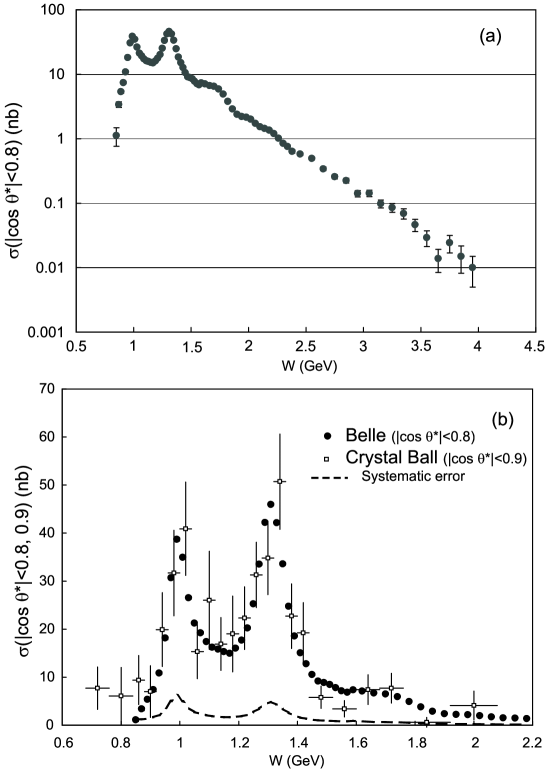
Figure 9: The cross section integrated over $|\cos\theta^{*}|<0.8$ on a logarithmic (a) and linear (b) scale compared with the Crystal Ball measurement ($|\cos\theta^{*}|<0.9$) cbep . The corrections for different $|\cos\theta^{*}|$ coverage are not made. The dashed curve shows the size of the systematic error.

III.5 Systematic errors

Various sources of systematic uncertainties assigned for the $\eta\pi^{0}$ signal yield, efficiency and the cross section evaluation are described in detail below and summarized in Table 3.

Trigger efficiency: The systematic error due to the Clst4 trigger (the mnemonics of the ECL triggers were described in Sec. II.A) is taken to be $2/3$ of the difference in the efficiencies when the thresholds for the Clst4 trigger are varied from 110 MeV to 100 MeV in the trigger simulator, and no error is assigned for $W>2.5$ GeV where the HiE trigger plays a dominant role. In addition, we take the uncertainty in the efficiency of the HiE trigger to be 4% in the whole $W$ region. The systematic errors from the two triggers are combined in quadrature. The former component is approximated by an angular-independent function of the c.m. energy, $27\%\times 0.5^{10(W-0.85~{}[{\rm GeV}])}$. This exceeds 5% for $W<1.2$ GeV.

The reconstruction efficiency: we assign 6% for the reconstruction of a $\pi^{0}$ and an $\eta$.

$p_{t}$-balance cut: 3% is assigned. The $p_{t}$-balance distribution for the signal is well reproduced by MC so that the efficiency is correct to within this error.

Background subtraction: 20% of the size of the subtracted component is assigned to this source for the range $0.9~{}{\rm GeV}<W<2.0~{}{\rm GeV}$. In the $W$ region where the background subtraction is not applied ($W>2.0$ GeV), we assign a systematic error of 3%, which is a conservative upper limit on the background contamination from an investigation of the experimental distributions. Above 3.5 GeV, the error originating from the background subtraction ($\Delta R/12$) is larger than 3%, and we replace the error by the latter value. In the region $0.84~{}{\rm GeV}<W<0.90~{}{\rm GeV}$ where the $\eta^{\prime}$ background is subtracted, the assigned error is a quadratic sum of 7% of the subtracted $\eta^{\prime}$ background and 20% of the subtracted $p_{t}$-unbalanced background.

Luminosity function: We assign 4% (5%) for $W<\;(>)\;3.0$ GeV.

Beam background effect for event selection: We assign a 2% - 6% error depending on $W$ for uncertainties of the inefficiency in event selection due to beam-background photons. The uncertainty is estimated from the variation of efficiencies among different experimental periods or background conditions. We adopt the averaged efficiency from the different background files, and the uncertainty in the average is assigned as the error.

Unfolding: Uncertainties from the unfolding procedure, using the single value decomposition approach in Ref. svdunf , are estimated by varying the effective-rank parameter of the decomposition within reasonable bounds.

Other efficiency errors: An error of 4% is assigned for uncertainties in the efficiency determination based on MC including the smoothing procedure.

The total systematic error is obtained by adding all the sources in quadrature and is 10-12% for the intermediate and high $W$ regions. It becomes much larger for $W<1.06~{}{\rm GeV}$.

Table 3: Systematic errors for the differential cross sections. Ranges of errors are shown when they depend on $W$.

Source	Error (%)
Trigger efficiency	4 – 30
$\eta$ and $\pi^{0}$ reconstruction efficiency	6
$p_{t}$-balance cut	3
Background subtraction	3 – 35
Luminosity function	4 – 5
Overlapping hits from beam background	2 – 6
Unfolding procedure	0 – 4
Other efficiency errors	4
Overall	10 – 12 (for $W>1.06~{}{\rm GeV}$)

IV Study of resonances

In this section, we extract the resonance parameters of the $a_{0}(980)$ and a possible resonance $a_{0}(1450)$, as well as check the consistency of the $a_{2}(1320)$ parameters. We also study whether or not the $a_{2}(1700)$ is produced in this reaction.

IV.1 Formalism

The formalism is exactly the same as that for $\pi\pi$ mori1 ; mori2 ; pi0pi0 ; pi0pi02 and the analysis is quite similar. In the energy region $W\leq 2.0~{}{\rm GeV}$, $J>2$ partial waves (the next is $J=4$) may be neglected so that only S and D waves are to be considered. The differential cross section can be expressed as:

$$\frac{d\sigma}{d\Omega}(\gamma\gamma\to\eta\pi^{0})=\left|S\>Y^{0}_{0}+D_{0}\>Y^{0}_{2}\right|^{2}+\left|D_{2}\>Y^{2}_{2}\right|^{2}\;,$$ (4)

where $S$ represents the S wave, $D_{0}$ ($D_{2}$) denotes the helicity 0 (2) components of the D wave, respectively, and $Y^{m}_{J}$ are the spherical harmonics. Since the $|Y^{m}_{J}|$’s are not independent of each other, partial waves cannot be separated using measurements of differential cross sections alone. To overcome this problem, we write Eq. (4) as:

$$\frac{d\sigma}{4\pi d|\cos\theta^{*}|}(\gamma\gamma\to\eta\pi^{0})=\hat{S}^{2}\>|Y^{0}_{0}|^{2}+\hat{D}_{0}^{2}\>|Y^{0}_{2}|^{2}+\hat{D}_{2}^{2}\>|Y^{2}_{2}|^{2}\,.$$ (5)

The amplitudes $\hat{S}^{2}$, $\hat{D}_{0}^{2}$ and $\hat{D}_{2}^{2}$ correspond to the cases where interference terms are neglected; they can be expressed in terms of $S,~{}D_{0}$ and $D_{2}$ as follows pi0pi0 :

$$\hat{S}^{2} = |S|^{2}+\sqrt{5}{\rm Re}{(S^{*}D_{0})}\;,$$

$$\hat{D}_{0}^{2} = |D_{0}|^{2}+\frac{1}{\sqrt{5}}{\rm Re}{(S^{*}D_{0})}\;,$$

$$\hat{D}_{2}^{2} = |D_{2}|^{2}-\frac{6}{\sqrt{5}}{\rm Re}{(S^{*}D_{0})}\;.$$ (6)

Since squares of spherical harmonics are independent of each other, we can fit the differential cross section at each $W$ to obtain $\hat{S}^{2}$, $\hat{D}_{0}^{2}$, and $\hat{D}_{2}^{2}$. The unfolded differential cross sections are fitted by taking into account statistical errors only, which will not be independent at each $W$ because of the unfolding procedure. However, we treat them as independent in the fit. The resulting $\hat{S}^{2}$, $\hat{D}_{0}^{2}$ and $\hat{D}_{2}^{2}$ spectra for $W<2~{}{\rm GeV}$ are shown in Figs. 10.

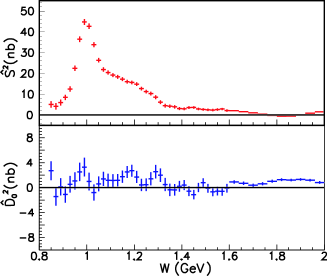
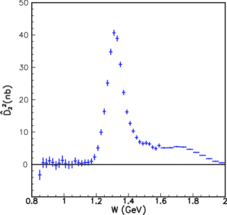
Figure 10: Resulting spectra of $\hat{S}^{2}$, $\hat{D}_{0}^{2}$ and $\hat{D}_{2}^{2}$. The error bars shown are diagonal statistical errors.

IV.2 Fitting partial wave amplitudes

Although the derived amplitudes $\hat{S}^{2}$, $\hat{D}_{0}^{2}$ and $\hat{D}_{2}^{2}$ are functions of partial waves (Eq. (6)), they do give some indication of their behavior. Notably, the D₀ wave appears to be small and the D₂ wave is dominated by the $a_{2}(1320)$ with a hint of the $a_{2}(1700)$. The peak in $\hat{S}^{2}$ around $W=0.98~{}{\rm GeV}$ (Fig. 10) is clearly due to the $a_{0}(980)$ resonance and a shoulder above the $a_{0}(980)$ peak may be due to the $a_{0}(1450)$.

In this section, we derive information about resonances by parameterizing partial wave amplitudes and fitting differential cross sections. Note that we do not fit the obtained $\hat{S}^{2}$, $\hat{D}_{0}^{2}$ and $\hat{D}_{2}^{2}$ spectra but fit the differential cross sections directly. Once the functional forms of amplitudes are assumed, we can use Eq. (4) to fit differential cross sections. We can then neglect the correlations between $\hat{S}^{2}$, $\hat{D}_{0}^{2}$ and $\hat{D}_{2}^{2}$. The $\hat{S}^{2}$, $\hat{D}_{0}^{2}$ and $\hat{D}_{2}^{2}$ spectra are used to make an initial determination of which resonances are important and to check fit quality.

The energy range of this measurement can be naturally divided into a low energy region ($W\leq 1.5~{}{\rm GeV}$), where the $a_{0}(980)$ and $a_{2}(1320)$ are important, and a higher energy region ($W>1.5~{}{\rm GeV}$), where the parameters of the $a_{2}(1700)$ will be of interest. In both regions, we neglect $J>2$ waves.

First we extract parameters of the $a_{2}(1700)$ in the high energy range. A hint of the $a_{2}(1700)$ is visible in Fig. 9. Various fits have been performed: a fit in the energy region $1.5~{}{\rm GeV}<W<2.0~{}{\rm GeV}$ with the parameters of the $a_{2}(1700)$ all floated or the mass and width fixed to the PDG values; a fit in the energy region $0.9~{}{\rm GeV}<W<2.0~{}{\rm GeV}$ by fixing the lower energy parameters to the ones determined below and either floating or partially fixing the parameters of the $a_{2}(1700)$. The resulting parameters of the $a_{2}(1700)$ vary much. In addition, the fit quality is poor. Thus, we cannot report a definite conclusion on the $a_{2}(1700)$.

In the low energy region, $W<1.5~{}{\rm GeV}$, we can safely neglect $J>2$ waves. The $\hat{D}_{0}^{2}$ contribution is small while $\hat{D}_{2}^{2}$ is seen to be dominated by the $a_{2}(1320)$ resonance. We assume that the $a_{2}(1320)$ contributes to the $D_{2}$ wave only, since $\hat{D}_{0}^{2}$ is small. The shoulder in the $\hat{S}^{2}$ spectrum above the $a_{0}(980)$ peak may be due to the $a_{0}(1450)$. However, in this fit we introduce a new resonance $a_{0}(Y)$ instead, since its parameters are found to be quite different from those of the $a_{0}(1450)$. The goal of analysis is to obtain parameters of the $a_{0}(980)$, $a_{0}(Y)$ and to check the consistency of the $a_{2}(1320)$ parameters that have been measured well in the past.

IV.2.1 Parameterization of amplitudes

We parameterize $S$, $D_{0}$ and $D_{2}$ waves as follows.

$$S = A_{a_{0}(980)}e^{i\phi_{s0}}+A_{a_{0}(Y)}e^{i\phi_{s1}}+B_{S}\;,$$

$$D_{0} = B_{D0}\;,$$

$$D_{2} = A_{a_{2}(1320)}e^{i\phi_{d2}}+B_{D2}\;,$$ (7)

where $A_{a_{0}(980)}$, $A_{a_{0}(Y)}$ and $A_{a_{2}(1320)}$ are the amplitudes of the $a_{0}(980)$, $a_{0}(Y)$ and $a_{2}(1320)$, respectively; $B_{S}$, $B_{D0}$ and $B_{D2}$ are non-resonant (called hereafter “background”) amplitudes for S, D₀ and D₂ waves; and $\phi_{s0}$, $\phi_{s1}$, and $\phi_{d2}$ are the phases of resonances relative to background amplitudes. We also study the case with no $a_{0}(Y)$ and the case with the mass of the $a_{0}(Y)$ fixed to that of the $a_{0}(1450)$.

The background amplitudes are parameterized as follows.

$$B_{S} = a_{s}W^{\prime 2}+b_{s}W^{\prime}+c_{s}+i(a^{\prime}_{s}W^{\prime 2}+b^{\prime}_{s}W^{\prime}+c^{\prime}_{s}),$$

$$B_{D0} = a_{0}W^{\prime 2}+b_{0}W^{\prime}+c_{0}+i(a^{\prime}_{0}W^{\prime 2}+b^{\prime}_{0}W^{\prime}+c^{\prime}_{0}),$$

$$B_{D2} = a_{2}W^{\prime 2}+b_{2}W^{\prime}+c_{2}+i(a^{\prime}_{2}W^{\prime 2}+b^{\prime}_{2}W^{\prime}+c^{\prime}_{2}).$$ (8)

Here $W^{\prime}=W-W_{\rm th}$ where $W_{\rm th}$ is the threshold energy. We assume background amplitudes to be quadratic in $W$ for the both real and imaginary parts of all waves. In this way, symmetries among amplitudes are kept. The arbitrary phases are fixed by choosing $\phi_{s0}=\phi_{d2}=0$. We constrain all the background amplitudes to be zero at the threshold by setting the $c$ and $c^{\prime}$ parameters to zero in accordance with the expectation that the cross section vanishes at the Thomson limit.

The relativistic Breit-Wigner resonance amplitude $A_{R}(W)$ for a spin-$J$ resonance $R$ of mass $m_{R}$ is given by

$$A_{R}^{J}(W) = \sqrt{\frac{8\pi(2J+1)m_{R}}{W}}\frac{\sqrt{\Gamma_{\rm tot}(W)\Gamma_{\gamma\gamma}(W){{\cal B}}(\eta\pi^{0})}}{m_{R}^{2}-W^{2}-im_{R}\Gamma_{\rm tot}(W)}\;,$$ (9)

The energy-dependent total width $\Gamma_{\rm tot}(W)$ is given by

$$\Gamma_{\rm tot}(W)=\sum_{X}\Gamma_{X_{1}X_{2}}(W)\;,$$ (10)

where $X_{i}$ is $\pi$, $K$, $\eta$, $\gamma$, etc. For $J=2$ (the $a_{2}(1320)$ meson), the partial width $\Gamma_{X_{1}X_{2}}(W)$ is parameterized as blat :

$$\Gamma_{X_{1}X_{2}}(W)=\Gamma_{R}{\cal B}(R\rightarrow X_{1}X_{2})\left(\frac{q_{X}(W^{2})}{q_{X}(m_{R}^{2})}\right)^{5}\frac{D_{2}\left(q_{X}(W^{2})r_{R}\right)}{D_{2}\left(q_{X}(m_{R}^{2})r_{R}\right)}\;,$$ (11)

where $\Gamma_{R}$ is the total width at the resonance mass, $q_{X}(W^{2})=\sqrt{(W^{2}-(m_{X_{1}}+m_{X_{2}})^{2})(W^{2}-(m_{X_{1}}-m_{X_{2}})^{2})}/(2W)$, $D_{2}(x)=1/(9+3x^{2}+x^{4})$, and $r_{R}$ is an effective interaction radius that varies from 1 ${\rm GeV}^{-1}$ to 7 ${\rm GeV}^{-1}$ in different hadronic reactions grayer . For the three-body and the other decay modes, $\Gamma_{3-{\rm body}}(W)=\Gamma_{R}{\cal B}(R\rightarrow 3-{\rm body})\frac{W^{2}}{m_{R}^{2}}$ is used instead of Eq. (11). All the parameters of the $a_{2}(1320)$ are fixed to the PDG values as listed in Table 4 pdg , except for $r_{R}$ which is fitted to be $3.09^{+0.53}_{-0.55}~{}({\rm GeV}/c)^{-1}$, consistent with $3.62\pm 0.03~{}({\rm GeV}/c)^{-1}$ determined for the $f_{2}(1270)$ mori2 . For the $a_{0}(980)$ and $a_{0}(Y)$, the widths are taken to be energy independent. For the $a_{0}(980)$, a simple Breit-Wigner formula is used instead of the more sophisticated formula used in Ref. mori1 ; mori2 for the $f_{0}(980)$. This is because the resonance shape appears to be symmetric with no indication of the effect of the $K\bar{K}$ threshold. In fact, a fit with the formula in Ref. mori1 ; mori2 gives $g^{2}_{K\bar{K}}/g^{2}_{\eta\pi}=0^{+0.03}_{-0}$, where $g_{KK}$ ($g_{\pi\pi}$) is the coupling of the $a_{0}(980)$ to $K\bar{K}$ ($\pi\pi$).

Table 4: Parameters of the $a_{2}(1320)$ pdg .

Parameter	Value	Unit
Mass	$1318.3\pm 0.6$	${\rm MeV}/c^{2}$
$\Gamma_{\rm tot}$	$107\pm 5$	MeV
${\cal B}({a_{2}\rightarrow\rho\pi})$	$70.1\pm 2.7$	%
${\cal B}({a_{2}\rightarrow\eta\pi})$	$14.5\pm 1.2$	%
${\cal B}({a_{2}\rightarrow\omega\pi\pi})$	$10.6\pm 3.2$	%
${\cal B}({a_{2}\rightarrow K\bar{K}})$	$4.9\pm 0.8$	%
${\cal B}({a_{2}\rightarrow\gamma\gamma})$	$(9.4\pm 0.7)\times 10^{-6}$	–

IV.2.2 Fitted parameters

We fit differential cross sections with the parameterized amplitudes for the range $0.90~{}{\rm GeV}\leq W\leq 1.46~{}{\rm GeV}$. There are 19 parameters to be fitted. About one thousand sets of randomly generated initial parameters are prepared and fitted using MINUIT minuit to search for the true minimum and to find any multiple solutions. A unique solution is found with $\chi^{2}/ndf=597.6/429=1.39$ ($ndf$ denotes the number of degrees of freedom) for the nominal fit, which appears in more than $\sim 3$% of the cases. The fitted parameters are listed in Table 5. The quoted errors are MINOS statistical errors. They are calculated from the $\chi^{2}$ values obtained by varying each parameter while floating all the other parameters.

Table 5: Fitted parameters. The errors are statistical only.

Resonance	Parameter	Nominal	$M(a_{0}(Y))$ fixed	No $a_{0}(Y)$	Unit
$a_{0}(980)$	Mass	$982.3^{+0.6}_{-0.7}$	$982.3^{+0.8}_{-0.7}$	$982.3\pm 0.6$	MeV/$c^{2}$
	$\Gamma_{\rm tot}$	$75.6\pm 1.6$	$76.9^{+1.0}_{-1.3}$	$75.6^{+1.4}_{-1.3}$	MeV
	$\Gamma_{\gamma\gamma}{\cal B}(\eta\pi^{0})$	$128^{+3}_{-2}$	$558^{+52}_{-44}$	$642\pm 8$	eV
$a_{0}(Y)$	Mass	$1316.8^{+0.7}_{-1.0}$	1474.0 (fixed)	–	MeV/$c^{2}$
	$\Gamma_{\rm tot}$	$65.0^{+2.1}_{-5.4}$	$251^{+25}_{-33}$	–	MeV
	$\Gamma_{\gamma\gamma}{\cal B}(\eta\pi^{0})$	$432\pm 6$	$(11.0^{+4.4}_{-3.3})\times 10^{3}$	0 (fixed)	eV
$\chi^{2}/ndf$		597.6/429=1.39	704.5/430=1.65	753.6/433=1.74

Differential cross sections together with the fitted curves are shown in Fig. 11 for selected $W$ bins. The fit is reasonable as can be seen from these bins and from Fig. 12, where the quantities $\hat{S}^{2}$ and $\hat{D}_{2}^{2}$ are reproduced reasonably well.

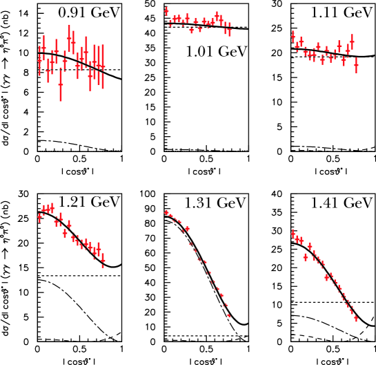
Figure 11: Differential cross section ($d\sigma/d|\cos\theta^{*}|$ (nb)) (data points) and results of the fit (solid line) for the $W$ bins indicated. The dotted, dashed and dot-dashed curves indicate the $|S|^{2}$, $4\pi|D_{0}Y_{2}^{0}|^{2}$ and $4\pi|D_{2}Y_{2}^{2}|^{2}$ contributions, respectively.

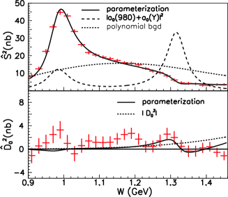
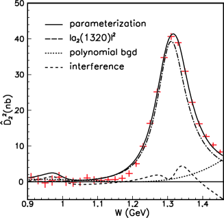
Figure 12: Results of the parameterization and $\hat{S}^{2}$ (left top), $\hat{D}_{0}^{2}$ (left bottom), and $\hat{D}_{2}^{2}$ (right). The error bars shown are diagonal statistical error.

The total cross section ($|\cos\theta^{*}|<0.8$) can be obtained by integrating Eq. (5) as:

$$\sigma_{\rm tot}=0.8\hat{S}^{2}+0.457\hat{D}_{0}^{2}+0.983\hat{D}_{2}^{2}\;,$$ (12)

where the factors come from the integration of spherical harmonics for $|\cos\theta^{*}|\leq 0.8$. The measured total cross section is in good agreement with the prediction obtained from the sum of the fitted amplitudes as shown in Fig. 13.

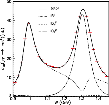
Figure 13: Total cross section ($|\cos\theta^{*}|<0.8$) and results of the parameterization. Contributions of $|S|^{2},\;|D_{0}|^{2}$ and $|D_{2}|^{2}$ (not $\hat{S}^{2}$, $\hat{D}_{0}^{2}$ and $\hat{D}_{2}^{2}$) are also shown.

So far we have used the measured parameter values for the $a_{2}(1320)$. However, having high statistics two-photon production data, one might question their validity, in particular, ${\cal B}(a_{2}(1320)\rightarrow\gamma\gamma)$. Namely, the determination of this quantity may have been biased in past experiments by the presence of non-resonant background, etc. To study this effect, a fit is performed where the product $\Gamma_{\gamma\gamma}{\cal B}(\eta\pi^{0})$ of the $a_{2}(1320)$ is also floated. The value $\Gamma_{\gamma\gamma}(a_{2}(1320)){\cal B}(\eta\pi^{0})$ obtained is $(145^{+97}_{-34})$ eV, which corresponds to ${\cal B}(a_{2}(1320)\rightarrow\gamma\gamma)=(9.4^{+6.3}_{-2.2})\times 10^{-6}$; it agrees well with the PDG value, $(9.4\pm 0.7)\times 10^{-6}$ within the rather large fitting error. Thus, we conclude that the parameters obtained in past measurements are reasonable. The large statistical error in our measurement arises because of interference.

The $a_{0}(Y)$ mass is close to that of the $a_{2}(1320)$, which may suggest the possibility that the $a_{0}(Y)$ is just a contribution of the $a_{2}(1320)$ to the D₀ wave, which is not taken into account in the above fit. To test this hypothesis, a fit is performed with the $a_{0}(Y)$ removed and with $D_{0}$ and $D_{2}$ in Eq. (7) replaced by

$$D_{0} = \sqrt{\frac{r_{02}}{1+r_{02}}}A_{a_{2}(1320)}e^{i\phi_{d0}}+B_{D0}\;,$$

$$D_{2} = \sqrt{\frac{1}{1+r_{02}}}A_{a_{2}(1320)}e^{i\phi_{d2}}+B_{D2}\;,$$ (13)

where $r_{02}$ indicates the fraction of the $a_{2}(1320)$ in the D₀ wave. We obtain $r_{02}=1.7^{+0.5}_{-0.4}$% with $\chi^{2}/ndf=737.7/431$. The fit quality is unacceptably poor. When the $a_{0}(Y)$ is restored and a fit is performed with Eq. (13), we obtain $r_{02}=3.4^{+2.3}_{-1.1}$% with $\chi^{2}/ndf=580.6/427$. We conclude that the contribution of the $a_{2}(1320)$ to the D₀ wave is small.

The mass and width of the $a_{0}(Y)$ are significantly smaller than $1474\pm 19~{}{\rm MeV}/c^{2}$ and $265\pm 13~{}{\rm MeV}$, the parameters of the $a_{0}(1450)$ in the PDG pdg . Since the fit without the $a_{0}(Y)$ or one where the mass of the $a_{0}(Y)$ fixed to the $a_{0}(1450)$ mass are unacceptable (Table 5), the inclusion of the $a_{0}(Y)$ is required to explain the structure in $\hat{S}^{2}$ near 1.3 GeV seen in Fig. 12. Since, the mass and width of the $a_{0}(1450)$ are far from established, we may either identify the $a_{0}(Y)$ with the $a_{0}(1450)$ or treat it as another scalar resonance.

IV.2.3 Study of systematic errors

The following sources of systematic errors on the parameters are considered: dependence on the fitted region, normalization errors in the differential cross sections, assumptions about the background amplitudes, uncertainties from the unfolding procedure, and the uncertainties of the $a_{2}(1320)$. For each study, a fit is performed allowing all the parameters to float and the differences of the fitted parameters from the nominal values are quoted as systematic errors. A thousand sets of randomly prepared input parameters are prepared for each study and fitted to search for the true minimum and for possible multiple solutions. Unique solutions are found very often.

Two fitting regions are tried: higher ($0.94~{}{\rm GeV}\leq W\leq 1.50~{}{\rm GeV}$) and lower ($0.86~{}{\rm GeV}\leq W\leq 1.42~{}{\rm GeV}$). Normalization error studies are divided into those from uncertainties of overall normalization and those from distortion of the spectra in either $|\cos\theta^{*}|$ or $W$. For overall normalization errors, fits are made with two sets of values of differential cross sections obtained by multiplying by $(1\pm\sigma_{\epsilon(W,|\cos\theta^{*}|)})$, where $\sigma_{\epsilon}$ is the relative efficiency error; the results are denoted “normalization” errors. For distortion studies, $\pm 4$% errors are assigned and differential cross sections are distorted by multiplying them by $(1\pm 0.1|\cos\theta^{*}|\mp 0.04)$ and $(1\pm(W({\rm GeV})-1.18)/7)$ (referred to as “bias:$|\cos\theta^{*}|$” and “bias:$W$” errors, respectively).

For studies of background (BG) amplitudes, one of the waves is changed to a first- or a third-order polynomial. In addition, constant terms are fixed to non-zero values. Uncertainties from the unfolding procedure are studied by analyzing the differential cross sections where a key parameter in unfolding is varied within an allowable range. Finally, the parameters of the $a_{2}(1320)$ are successively varied by their $\pm 1\sigma$ uncertainties.

The resulting systematic errors are summarized in Table 6. The total systematic errors are calculated by combining the individual errors in quadrature. As can be seen in Table 6, the values of $\Gamma_{\gamma\gamma}{\cal B}(\eta\pi^{0})$ for the $a_{0}(980)$ and $a_{0}(Y)$ jump to much larger values in some of the systematic variations. This is because destructive interference is preferred in some of the studies. A study reveals that for much narrower $W$ regions, e.g. about the $a_{0}(980)$ peak region, there exist two solutions corresponding to constructive and destructive interference; the latter solution is disfavored in a wider $W$ range in the nominal fit, but favored in some of the systematic studies. In this case, taking the sum in quadrature of the individual errors will be an overestimation. Thus, we choose the maximum deviation among the different systematic variations to estimate the total systematic error.

Table 6: Systematic uncertainties for $a_{0}(980)$ and $a_{0}(Y)$ parameters

	$a_{0}(980)$			$a_{0}(Y)$
Source	Mass	$\Gamma_{\rm tot}$	$\Gamma_{\gamma\gamma}{\cal B}(\eta\pi^{0})$	Mass	$\Gamma_{\rm tot}$	$\Gamma_{\gamma\gamma}{\cal B}_{\eta\pi 0}$
	(MeV/$c^{2}$)	(MeV)	(eV)	(MeV/$c^{2}$)	(MeV)	(eV)
$W$ fit range	${}^{+0.4}_{-1.1}$	${}^{+2.4}_{-0.0}$	${}^{+7.9}_{-0.0}$	${}^{+5.7}_{-1.2}$	${}^{+4.3}_{-2.7}$	${}^{+0.0}_{-57.0}$
Normalization	${}^{+0.4}_{-0.6}$	${}^{+0.2}_{-0.2}$	${}^{+17.6}_{-19.5}$	${}^{+0.9}_{-0.0}$	${}^{+0.0}_{-1.3}$	${}^{+20.2}_{-46.4}$
Bias:$|~{}\cos~{}\theta^{|}$	${}^{+0.0}_{-0.1}$	${}^{+0.4}_{-0.2}$	${}^{+0.0}_{-9.3}$	${}^{+3.6}_{-0.0}$	${}^{+6.6}_{-18.1}$	${}^{+0.0}_{-179.3}$
Bias:$W$	${}^{+0.0}_{-0.1}$	${}^{+0.2}_{-0.1}$	${}^{+5.1}_{-4.6}$	${}^{+0.1}_{-0.0}$	${}^{+0.5}_{-0.5}$	${}^{+0.8}_{-1.4}$
BG:${\rm Re}(S)$ param.	${}^{+2.9}_{-0.5}$	${}^{+0.0}_{-1.4}$	${}^{+0.0}_{-10.6}$	${}^{+0.0}_{-0.8}$	${}^{+12.2}_{-0.9}$	${}^{+150.2}_{-35.0}$
BG:${\rm Im}(S)$ param.	${}^{+0.0}_{-1.6}$	${}^{+0.5}_{-0.6}$	${}^{+482.4}_{-6.1}$	${}^{+17.3}_{-0.0}$	${}^{+97.8}_{-6.8}$	${}^{+1061.1}_{-141.5}$
BG:${\rm Re}(S)\;c\neq 0$	${}^{+0.1}_{-0.5}$	${}^{+0.1}_{-0.3}$	${}^{+0.0}_{-9.3}$	${}^{+0.1}_{-0.1}$	${}^{+0.0}_{-0.4}$	${}^{+0.0}_{-12.0}$
BG:${\rm Re}(D_{0})$ param.	${}^{+0.0}_{-0.9}$	${}^{+0.0}_{-0.3}$	${}^{+0.0}_{-2.0}$	${}^{+6.6}_{-0.0}$	${}^{+1.9}_{-10.2}$	${}^{+18.1}_{-215.7}$
BG:${\rm Im}(D_{0})$ param.	${}^{+0.0}_{-0.9}$	${}^{+0.0}_{-0.3}$	${}^{+0.0}_{-2.0}$	${}^{+6.6}_{-0.0}$	${}^{+0.0}_{-10.3}$	${}^{+0.0}_{-215.7}$
BG:${\rm Re}(D_{0})\;c\neq 0$	${}^{+0.3}_{-0.7}$	${}^{+0.3}_{-0.0}$	${}^{+0.0}_{-9.4}$	${}^{+6.6}_{-0.0}$	${}^{+0.3}_{-14.4}$	${}^{+0.0}_{-229.6}$
BG:${\rm Re}(D_{2})$ param.	${}^{+0.0}_{-0.1}$	${}^{+0.5}_{-0.0}$	${}^{+0.0}_{-6.3}$	${}^{+5.4}_{-0.0}$	${}^{+0.0}_{-13.4}$	${}^{+0.0}_{-210.8}$
BG:${\rm Im}(D_{2})$ param.	${}^{+0.0}_{-0.0}$	${}^{+0.0}_{-0.0}$	${}^{+0.2}_{-3.0}$	${}^{+0.6}_{-0.0}$	${}^{+0.0}_{-1.3}$	${}^{+0.0}_{-18.4}$
BG:${\rm Re}(D_{2})\;c\neq 0$	${}^{+0.5}_{-0.0}$	${}^{+0.5}_{-0.0}$	${}^{+3.9}_{-0.6}$	${}^{+0.6}_{-0.0}$	${}^{+1.2}_{-0.3}$	${}^{+11.7}_{-6.6}$
Unfolding	${}^{+0.7}_{-3.9}$	${}^{+17.2}_{-9.8}$	${}^{+501.2}_{-31.3}$	${}^{+9.7}_{-3.2}$	${}^{+0.0}_{-7.4}$	${}^{+0.0}_{-213.3}$
$a_{2}$:mass	${}^{+0.0}_{-0.1}$	${}^{+0.1}_{-0.1}$	${}^{+0.7}_{-0.8}$	${}^{+0.9}_{-0.9}$	${}^{+0.0}_{-0.3}$	${}^{+0.7}_{-5.6}$
$a_{2}$:width	${}^{+0.2}_{-0.2}$	${}^{+1.0}_{-0.8}$	${}^{+3.9}_{-4.1}$	${}^{+2.7}_{-2.8}$	${}^{+5.4}_{-4.7}$	${}^{+48.0}_{-38.9}$
$a_{2}:\Gamma_{\gamma\gamma}{\cal B}(\eta\pi^{0})$	${}^{+0.0}_{-0.1}$	${}^{+0.1}_{-0.0}$	${}^{+0.7}_{-0.6}$	${}^{+1.1}_{-0.6}$	${}^{+0.7}_{-1.6}$	${}^{+12.2}_{-25.3}$
$a_{2}:r_{R}$	${}^{+0.3}_{-0.0}$	${}^{+0.4}_{-0.0}$	${}^{+5.3}_{-0.0}$	${}^{+0.4}_{-0.3}$	${}^{+2.6}_{-1.6}$	${}^{+8.4}_{-10.9}$
Total	${}^{+3.1}_{-4.7}$	${}^{+17.4}_{-10.0}$	${}^{+501.6}_{-43.0}$	${}^{+24.7}_{-4.6}$	${}^{+99.1}_{-32.6}$	${}^{+1073.2}_{-255.5}$

IV.2.4 Summary of resonance studies

To summarize the study presented in this section, once the amplitudes are parameterized, differential cross sections can be fitted to obtain the parameters as described above. Although the fit itself is not very good as can be seen from $\chi^{2}/ndf=1.39$, it is stable despite the fact that the approach to the minimum is slow; tens of MINUIT runs are needed to reach the minimum. The mass, width and $\Gamma_{\gamma\gamma}{\cal B}(\eta\pi^{0})$ values obtained for the $a_{0}(980)$ and $a_{0}(Y)$ are summarized and compared to those in the PDG pdg in Tables 7 and 8. Note that the value of the product $\Gamma_{\gamma\gamma}{\cal B}(\eta\pi^{0})$ in the PDG pdg is an average of Refs. cbep and jade . In both analyses, the total cross section or an event distribution is fitted to an incoherent sum of the $a_{0}(980)$ and $a_{2}(1320)$ resonances (with the masses and widths fixed to the earlier PDG values oldpdg ) and nonresonant background because of the limited statistics available. In our fit, we fully take into account interference among amplitudes. When we follow the same procedure as in the previous analyses, which ignored possible interference, we reproduce their values with much better statistical errors.

Table 7: Fitted parameters of the $a_{0}(980)$

Parameter	This work	PDG	Unit
Mass	$982.3~{}^{+0.6}_{-0.7}~{}^{+3.1}_{-4.7}$	$984.7\pm 1.2$	${\rm MeV}/c^{2}$
$\Gamma_{\rm tot}$	$75.6~{}\pm 1.6~{}^{+17.4}_{-10.0}$	50 – 100	MeV
$\Gamma_{\gamma\gamma}{\cal B}(\eta\pi^{0})$	$128~{}^{+3}_{-2}~{}^{+502}_{-43}$	$240~{}^{+80}_{-70}$	eV

Table 8: Fitted parameters of the $a_{0}(Y)$ compared to those of the $a_{0}(1450)$

Parameter	This work	$a_{0}(1450)$ (PDG)	Unit
Mass	$1316.8~{}^{+0.7}_{-1.0}~{}^{+24.7}_{-4.6}$	$1474\pm 19$	${\rm MeV}/c^{2}$
$\Gamma_{\rm tot}$	$65.0~{}^{+2.1}_{-5.4}~{}^{+99.1}_{-32.6}$	$265\pm 13$	MeV
$\Gamma_{\gamma\gamma}{\cal B}(\eta\pi^{0})$	$432~{}\pm 6~{}^{+1073}_{-256}$	unknown	eV

V Analysis of the higher energy region

In this section, we study the angular dependence of the differential cross sections, $W$ dependence of the total cross section, and the ratio of cross sections for $\eta\pi^{0}$ to $\pi^{0}\pi^{0}$ production in the high energy region, $W>2.4~{}{\rm GeV}$.

V.1 Angular dependence

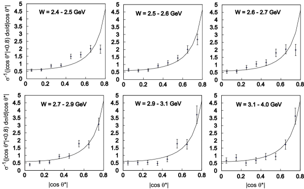
Figure 14: The angular dependence of the differential cross sections in different $W$ regions, with the normalization to the cross section integrated over $|\cos\theta^{*}|<0.8$. The curves are proportional to $\sin^{-4}\theta^{*}$ and normalized similarly.

As in the analysis of the $\pi^{0}\pi^{0}$ process pi0pi02 , we compare the angular dependence of the differential cross sections with the function $\sin^{-4}{\theta^{*}}$. A fit with an additional $\cos^{2}{\theta^{*}}$ term does not significantly improve the fit quality. Limited statistics prevent us from quantifying a possible deviation from the $\sin^{-4}{\theta^{*}}$ behavior when we study the $W$ dependence of the data. Here, we only show comparison with a $\sin^{-4}\theta^{*}$ parameterization in different $W$ regions in Fig. 14. In this figure, the vertical axis is the differential cross section divided by the total integral over $|\cos\theta^{*}|<0.8$. The curve is $0.602\sin^{-4}\theta^{*}$ (not a fit). The numerical factor is the differential cross section normalized to $\sigma(|\cos\theta^{*}|<0.8)$. The experimental result shows that the agreement is good for $W>2.7~{}{\rm GeV}$.

V.2 Power-law $W^{-n}$ dependence

We fit the $W$ dependence of the total cross section ($|\cos\theta^{*}|<0.8$) in the energy region 3.1-4.0 GeV, where the lower boundary 3.1 GeV is the same as in the $\pi^{0}\pi^{0}$ analysis. The fit gives $n=10.5\pm 1.2\pm 0.5$, and the corresponding cross section is drawn in Fig. 15(a) as well as that of the $\pi^{0}\pi^{0}$ process in the same angular range. The systematic error is obtained from the difference of the central values when we shift the cross section by $\pm 1\sigma$ at 3.1 GeV and $\mp 1\sigma$ at 4.0 GeV and by factors obtained by connecting linearly for $W$ bins in between, where $\sigma$ is an energy-dependent part of systematic error at each $W$ point. The $n$ value can be compared with $n$ values in other processes that we studied earlier nkzw ; wtchen ; pi0pi02 . The results are summarized in Table 9 from which it is clear that the result for the $\eta\pi^{0}$ final state is consistent with that for $K^{0}_{S}K^{0}_{S}$ (where the fitted $W$ range is wider), but two standard deviations higher than that for $\pi^{0}\pi^{0}$. The energy dependence of the latter seems to be different from that of the two other purely neutral final states and closer to $\pi^{+}\pi^{-}$ and $K^{+}K^{-}$, although no strict conclusions can be drawn at this level of statistics.

Table 9: The value of $n$ in $\sigma_{\rm tot}\propto W^{-n}$ in various reactions fitted in the $W$ and $|\cos\theta^{*}|$ ranges indicated.

Process	$n$	$W$ range (GeV)	$|\cos\theta^{*}|$ range	Reference
$\eta\pi^{0}$	$10.5\pm 1.2\pm 0.5$	3.1 – 4.1	$<0.8$	This work
$\pi^{0}\pi^{0}$	$8.0\pm 0.5\pm 0.4$	3.1 – 4.1 (exclude 3.3 – 3.6)	$<0.8$	pi0pi02
$K^{0}_{S}K^{0}_{S}$	$10.5\pm 0.6\pm 0.5$	2.4 – 4.0 (exclude 3.3 – 3.6)	$<0.6$	wtchen
$\pi^{+}\pi^{-}$	$7.9\pm 0.4\pm 1.5$	3.0 – 4.1	$<0.6$	nkzw
$K^{+}K^{-}$	$7.3\pm 0.3\pm 1.5$	3.0 – 4.1	$<0.6$	nkzw

V.3 Cross section ratio

A ratio of cross sections among neutral-pseudoscalar-meson ($\pi^{0}$ or $\eta$) pair production in two-photon collisions can be predicted relatively easily within a pQCD model. The pQCD model in Ref. bl predicts the cross section ratio $\sigma(\eta\pi^{0})/\sigma(\pi^{0}\pi^{0})$ as summarized in Table 10. In the table, $R_{f}=(f_{\eta}/f_{\pi^{0}})^{2}$, where $f_{\eta}$ ($f_{\pi}$) is the $\eta$ ($\pi^{0}$) form factor; the value of $R_{f}$ is not well known and we temporarily assume it to be unity. The ratio of the cross sections is proportional to the square of the coherent sum of the product of the quark charges, $|\Sigma e_{1}e_{2}|^{2}$, in which $e_{1}=-e_{2}$ in the present neutral-meson production cases. We show two predictions: a pure flavor SU(3) octet state and a mixture with $V_{P}=-18^{\circ}$ for the $\eta$ meson. For comparison, we also show in the table the values calculated using an incoherent sum as an example of an extreme case. Here, we assume that the quark-quark component of the neutral meson wave functions dominates and is much larger than the two-gluon component, in obtaining the relations between the cross sections.

Table 10: Predictions for the cross section ratio: $\sigma(\eta\pi^{0})/\sigma(\pi^{0}\pi^{0})$ in two-photon collisions. “Coherent sum” (“Incoherent sum”) is the ratio derived from the squared coherent (incoherent) sum of the product of the constituent-quark charges. Here, $R_{f}=(f_{\eta}/f_{\pi^{0}})^{2}$, where $f_{\eta}$ ($f_{\pi}$) is the $\eta$ ($\pi^{0}$) form factor; the value may be taken to be $R_{f}=1$. The $\eta$ meson is treated as a pure SU(3) octet state for the entries in the “octet” row, while “$V_{P}=-18^{\circ}$” is the most probable mixing angle between the octet and singlet states from experiments.

$\eta$ in SU(3)	Coherent sum	Incoherent sum
Octet	$0.24R_{f}$	$0.67R_{f}$
$V_{P}=-18^{\circ}$	$0.46R_{f}$	$1.29R_{f}$

The $W$ dependence of the ratio between the measured cross section integrated over $|\cos\theta^{*}|<0.8$ of $\gamma\gamma\to\eta\pi^{0}$ to $\gamma\gamma\to\pi^{0}\pi^{0}$ is plotted in Fig. 15(b). For the $\pi^{0}\pi^{0}$ process, the contributions from charmonium production are subtracted using a model-dependent assumption described in Ref. pi0pi02 . Even though the ratio may have a slight $W$ dependence, we average the ratio of the cross sections over the range $3.1~{}{\rm GeV}<W<4.0~{}{\rm GeV}$ as was done in other processes for the sake of comparison with QCD and obtain $0.48\pm 0.05\pm 0.04$. In the averaging, the ratio in the charmonium region (in $\pi^{0}\pi^{0}$) 3.3 - 3.6 GeV is not used. This ratio is in agreement with the QCD prediction if we take $R_{f}=1$.

V.4 Comments on charmonium

It is conjectured that the known $c\bar{c}$ charmonium states do not decay into the $\eta\pi^{0}$ final state with any observable rate, because the $I=1$ component should be suppressed. In other words, this process could be useful to search for a new charmonium-like particle with $I=1$ that would be a candidate for an exotic resonance. In Fig. 16, we show the invariant mass distribution of $\eta\pi^{0}$ events with $|\cos\theta^{*}|<0.4$, where a resonance contribution would be enhanced. We do not observe any signals of the known $\chi_{cJ}$ mesons. There is a hint of a peak near 3.18 GeV, however, its statistical significance is less than $3\sigma$. Therefore, we assumed in the above discussion that there are no charmonium contributions in the measurements of the cross section described here.

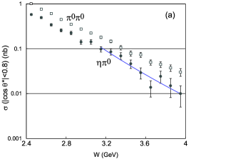
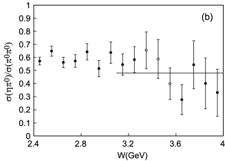
Figure 15: The $W$ dependence of the cross section ($|\cos\theta^{*}|<0.8$) (a). The curve is the power-law fit. The cross section of $\eta\pi^{0}$ production is compared to that for $\pi^{0}\pi^{0}$ pi0pi02 . The $W$ dependence of the cross section ratio of $\eta\pi^{0}$ to $\pi^{0}\pi^{0}$ ($|\cos\theta^{*}|<0.8$) (b). The line is the average in the 3.1 - 4.0 GeV range (the charmonium region, 3.3 - 3.6 GeV, is omitted from the calculation pi0pi02 ).

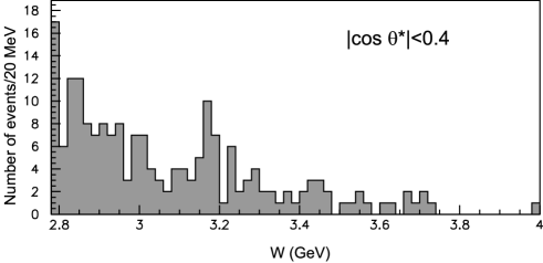
Figure 16: The $W$ distribution in the charmonium region ($|\cos\theta^{*}|<0.4$).

VI Summary and Conclusion

We have measured the process $\gamma\gamma\to\eta\pi^{0}$ using a high-statistics data sample from $e^{+}e^{-}$ collisions corresponding to an integrated luminosity of 223 fb^-1 with the Belle detector at the KEKB accelerator. We obtain results for the differential cross sections in the center-of-mass energy and polar angle ranges, $0.84~{}{\rm GeV}<W<4.0~{}{\rm GeV}$ and $|\cos\theta^{*}|<0.8$.

Differential cross sections are fitted in the energy region $0.90~{}{\rm GeV}\leq W\leq 1.46~{}{\rm GeV}$ in a model where partial waves consist of resonances and smooth backgrounds. The D₀ wave is small, the D₂ wave is dominated by the $a_{2}(1320)$ resonance, the S-wave prefers to have at least one additional resonance (denoted as $a_{0}(Y)$) in addition to the $a_{0}(980)$. The mass, width and the product $\Gamma_{\gamma\gamma}{\cal B}(\eta\pi^{0})$ for the $a_{0}(980)$ are fitted to be $982.3~{}^{+0.6}_{-0.7}~{}^{+3.1}_{-4.7}~{}{\rm MeV}/c^{2}$, $75.6~{}\pm 1.6~{}^{+17.4}_{-10.0}~{}{\rm MeV}$, $128~{}^{+3}_{-2}~{}^{+502}_{-43}~{}{\rm eV}$ and those for the $a_{0}(Y)$ are $1316.8~{}^{+0.7}_{-1.0}~{}^{+24.7}_{-4.6}~{}{\rm MeV}/c^{2}$, $65.0~{}^{+2.1}_{-5.4}~{}^{+99.1}_{-32.6}~{}{\rm MeV}$, $432~{}\pm 6~{}^{+1073}_{-256}~{}{\rm eV}$. The large systematic errors, in particular for two-photon widths, originate from an additional solution that favors destructive interference in some of systematic studies. The mass and width of the $a_{0}(Y)$ are significantly smaller than those of the $a_{0}(1450)$. The fact that the obtained $a_{0}(Y)$ mass is close to the $a_{2}(1320)$ mass may suggest that the $a_{2}(1320)$ contribution in the D₀ wave is important. However, a fit reveals that the fraction of the $a_{2}(1320)$ in the D₀ wave is small and it cannot replace the $a_{0}(Y)$. Since the fit without it or the fit where its mass is fixed to the $a_{0}(1450)$ mass is unacceptable, it is at least a good empirical parameterization. We may still identify the $a_{0}(Y)$ with the $a_{0}(1450)$, given that the latter is far from established, or as another new scalar meson. We cannot draw a definite conclusion on the existence of the $a_{2}(1700)$.

The angular distribution of the differential cross sections is close to $\sim\sin^{-4}\theta^{*}$ above $W=3.1$ GeV similarly to the $\pi^{0}\pi^{0}$. In this energy region, the energy dependence of the cross section integrated over $|\cos\theta^{*}|<0.8$ is well fitted by $W^{-n}$, $n=10.5\pm 1.5\pm 0.4$, somewhat higher (by two standard deviations) than that in the $\pi^{0}\pi^{0}$ channel. Although a slight $W$ dependence may remain in the ratio, we average the cross section ratio, $\sigma(\eta\pi^{0})/\sigma(\pi^{0}\pi^{0})$ in the range $3.1~{}{\rm GeV}<W<4.0~{}{\rm GeV}$ and obtain $0.48\pm 0.05\pm 0.04$. This ratio is consistent with the prediction from a QCD model based on $q\bar{q}$ production and SU(3) symmetry.

References

- (1) T. Mori et al. (Belle Collaboration), Phys. Rev. D 75, 051101(R) (2007).
- (2) T. Mori et al. (Belle Collaboration), J. Phys. Soc. Jpn 76, 074102 (2007).
- (3) H. Nakazawa et al. (Belle Collaboration), Phys. Lett. B 615, 39 (2005).
- (4) K. Abe et al. (Belle Collaboration), Eur. Phys. J. C 32, 323 (2004).
- (5) W.T. Chen et al. (Belle Collaboration), Phys. Lett. B 651, 15 (2007).
- (6) C.C. Kuo et al. (Belle Collaboration), Phys. Lett. B 621, 41 (2005).
- (7) S. Uehara et al. (Belle Collaboration), Phys. Rev. Lett. 96, 082003 (2006).
- (8) S. Uehara, Y. Watanabe et al. (Belle Collaboration), Phys. Rev. D 78, 052004 (2008).
- (9) S. Uehara, Y. Watanabe, H. Nakazawa et al. (Belle Collaboration), Phys. Rev. D 79, 052009 (2009).
-
(10)
See, e.g., the compilation in
http://durpdg.dur.ac.uk/spires/hepdata/online/2gamma/2gammahome.html. - (11) D. Antreasyan et al (Crystal Ball Collaboration), Phys. Rev. D 33, 1847 (1986).
- (12) See a latest review, “Light Scalar Mesons in Photon-Photon Collisions”, N.N. Achasov and G.N. Shestakov, arXiv:0905.2017v1 [hep-ph].
- (13) T. Oest et al. (JADE Collaboration), Z. Phys. C 47, 343 (1990).
- (14) S.K. Choi et al. (Belle Collaboration), Phys. Rev. Lett. 91, 262001 (2003); A. Abulencia et al. (CDF Collaboration), Phys. Rev. Lett. 96, 102002 (2008).
- (15) S.K. Choi et al. (Belle Collaboration), Phys. Rev. Lett. 100, 142001 (2008); R. Mizuk et al. (Belle Collaboration), Phys. Rev. D 78, 072004 (2008).
- (16) S.J. Brodsky and G.P. Lepage, Phys. Rev. D 24, 1808 (1981).
- (17) M. Diehl, P. Kroll and C. Vogt, Phys. Lett. B 532, 99 (2002).
- (18) A. Abashian et al. (Belle Collaboration), Nucl. Instr. and Meth. A 479, 117 (2002).
- (19) S. Kurokawa and E. Kikutani, Nucl. Instr. and. Meth. A 499, 1 (2003), and other papers included in this volume.
- (20) S. Uehara, KEK Report 96-11 (1996).
- (21) C. Amsler et al. (Particle Data Group), Phys. Lett. B 667, 1 (2008).
- (22) A. Höcker and V. Kartvelishvili, Nucl. Instr. Meth. A 372, 469 (1996).
- (23) J.M. Blatt and V.F. Weiskopff, Theoretical Nuclear Physics (Wiley, New York, 1952), pp. 359-365 and 386-389.
- (24) G. Grayer et al., Nucl. Phys. B 75, 189 (1974); A. Garmash et al. (Belle Collaboration), Phys. Rev. D 71, 092003 (2005); B. Aubert et al. (BaBar Collaboration), Phys. Rev. D 72, 052002 (2005).
- (25) F. James and M. Roos, Comput. Phys. Commun. 10, 343 (1975).
- (26) G.P. Yost et al. (Particle Data Group), Phys. Lett. 204 B, 1 (1988).