Algebraic methods for counting Euclidean embeddings of rigid graphs

Abstract

The study of (minimally) rigid graphs is motivated by numerous applications, mostly in robotics and bioinformatics. A major open problem concerns the number of embeddings of such graphs, up to rigid motions, in Euclidean space. We capture embeddability by polynomial systems with suitable structure, so that their mixed volume, which bounds the number of common roots, to yield interesting upper bounds on the number of embeddings. We focus on ${\mathbb{R}}^{2}$ and ${\mathbb{R}}^{3}$, where Laman graphs and 1-skeleta of convex simplicial polyhedra, respectively, admit inductive Henneberg constructions. We establish the first lower bound in ${\mathbb{R}}^{3}$ of about $2.52^{n}$, where $n$ denotes the number of vertices. Moreover, our implementation yields upper bounds for $n\leq 10$ in ${\mathbb{R}}^{2}$ and ${\mathbb{R}}^{3}$, which reduce the existing gaps, and tight bounds up to $n=7$ in ${\mathbb{R}}^{3}$.

Keywords: rigid graph, Euclidean embedding, Henneberg construction, polynomial system, lower bound, root bound, cyclohexane caterpillar

1 Introduction

Rigid graphs (or frameworks) constitute an old but still very active area of research due to their deep mathematical and algorithmic questions, as well as numerous applications, e.g. mechanism and linkage theory [12, 13], and structural bioinformatics [6, 9, 11].

Given a graph $G=(V,E)$ and a collection of edge lengths $l_{ij}\in{\mathbb{R}}^{+}$, for $(i,j)\in E$, a Euclidean embedding in $\mathbb{R}^{d}$ is a mapping of $V$ to a set of points in $\mathbb{R}^{d}$, such that $l_{ij}$ equals the Euclidean distance between the images of the $i$-th and $j$-th vertices, for $(i,j)\in E$. Euclidean embeddings impose no requirements on whether the edges cross each other or not. A graph is (generically) rigid in $\mathbb{R}^{d}$ iff, for generic (or random) edge lengths, it is embedded in ${\mathbb{R}}^{d}$ in a finite number of ways, modulo rigid motions. A graph is minimally rigid iff it is no longer rigid once any edge is removed.

A graph is called Laman iff $|E|=2|V|-3$ and, additionally, all of its induced subgraphs on $k<|V|$ vertices have $\leq 2k-3$ edges. The class of Laman graphs coincides with the generically minimally rigid graphs in $\mathbb{R}^{2}$, and also admit inductive constructions. In ${\mathbb{R}}^{3}$ there is no analogous combinatorial characterization of generically rigid graphs. On the other hand, the 1-skeleta, or edge graphs, of (convex) simplicial polyhedra are minimally rigid in $\mathbb{R}^{3}$, and admit inductive constructions, cf. Section 4.

In this paper, we deal with the problem of computing the maximum number of distinct planar and spatial Euclidean embeddings of (minimally) rigid graphs, up to rigid motions, as a function of the number of vertices. To study upper bounds, we define a square polynomial system, expressing the edge length constraints, whose real solutions correspond precisely to the different embeddings. Here is a system expressing embeddability in ${\mathbb{R}}^{3}$, where $(x_{i},y_{i},z_{i})$ are the coordinates of the $i$-th vertex, and 3 vertices are fixed to discard translations and rotations:

$$\small\left\{\begin{array}[]{ll}x_{i}=a_{i},\;y_{i}=b_{i},\;z_{i}=c_{i},&i=1,2,3,\quad a_{i},b_{i},c_{i}\in{\mathbb{R}},\\ (x_{i}-x_{j})^{2}+(y_{i}-y_{j})^{2}+(z_{i}-z_{j})^{2}=l_{ij}^{2},&(i,j)\in E-\{(1,2),(1,3),(2,3)\}\end{array}\right.$$ (1)

All nontrivial equations are quadratic; there are $2n-4$ for Laman graphs, and $3n-9$ for 1-skeleta of simplicial polyhedra, where $n$ is the number of vertices. The classical Bézout bound on the number of roots equals the product of the polynomials’ degrees, and yields $4^{n-2}$ and $8^{n-3}$, respectively. It is indicative of the hardness of the problem that efforts to substantially improve these bounds have failed.

For the planar and spatial case, the best known upper bounds are $\binom{2n-4}{n-2}\approx 4^{n-2}/\sqrt{\pi(n-2)}$ and $\frac{2^{n-3}}{n-2}\binom{2n-6}{n-3}\approx 8^{n-3}/\big{(}(n-2)\sqrt{\pi(n-3)}\big{)}$, respectively. These bounds were obtained using complex algebraic geometry [1, 2]. For ${\mathbb{R}}^{2}$, there exist lower bounds of $24^{\lfloor(n-2)/4\rfloor}\simeq 2.21^{n}$ and $2\cdot 12^{\lfloor(n-3)/3\rfloor}\simeq 2.29^{n}/6$, obtained by a caterpillar and a fan construction, respectively. Both of these bounds are based on the Desargues (or 3-prism) graph (Figure 2).

In applications, it is crucial to know the number of embeddings for specific (small) values of $n$. The most important result in this direction was to show that the Desargues graph admits 24 embeddings in the plane [2]. Moreover, the $K_{3,3}$ graph admits 16 embeddings in the plane [14, 12] and the cyclohexane graph admits 16 embeddings in space [6].

Mixed volume (or Bernstein’s bound) of a square polynomial system exploits the sparseness of the equations to bound the number of common roots, it is always bounded by Bézout’s bound and typically much tighter, cf. Section 3. We have implemented specialized software that constructs all rigid graphs up to isomorphism, for small $n$, and computes the mixed volumes of their respective polynomial systems. Our results indicate that mixed volume can be of general interest in enumeration problems.

Our main contribution is twofold, besides some straightforward upper bounds in Lemmas 2 and 3. First, we derive the first lower bound in ${\mathbb{R}}^{3}$:

$$16^{\lfloor(n-3)/3\rfloor}\simeq 2.52^{n},\,n\geq 9,$$

by designing a cyclohexane caterpillar.

Second, we obtain upper and lower bounds for $n\leq 10\$ in ${\mathbb{R}}^{2}$ and ${\mathbb{R}}^{3}$, which reduce the existing gaps, see Tables 1 and 2 in the Appendix. Moreover, we establish tight bounds up to $n=7$ in ${\mathbb{R}}^{3}$ by appropriately formulating the polynomial system. We apply Bernstein’s Second theorem to show that the naive polynomial system cannot yield tight mixed volumes, a fact already observed in the planar case [10].

The rest of the paper is structured as follows: Section 2 discusses the case $d=2$, Section 3 presents our algebraic tools and our implementation, Section 4 deals with ${\mathbb{R}}^{3}$, and we conclude with open questions and a conjecture. Omitted Figures and Tables have been included in the Appendix.

Some results appeared in [7] in preliminary form.

2 Planar embeddings of Laman graphs

Laman graphs admit inductive constructions that begin with a triangle, followed by a sequence of Henneberg-1 (or $H_{1}$) and Hennenerg-2 steps (or $H_{2}$). Each such step adds a new vertex as follows: a $H_{1}$ step connects it to two existing vertices; a $H_{2}$ step connects it to three existing vertices having at least one edge among them, which is removed (Figure 2). We represent each Laman graph by $\bigtriangleup s_{4}\ldots,s_{n}$, where $s_{i}\in\{1,2\}$; this is known as its Henneberg sequence. A Laman graph is called $H_{1}$ iff it can be constructed using only $H_{1}$ steps, and $H_{2}$ otherwise. Since two circles intersect generically in two points, a $H_{1}$ step at most doubles the number of embeddings and this is tight, generically. It follows that a $H_{1}$ graph on $n$ vertices has $2^{n-2}$ embeddings [2].

One can easily verify that every $\bigtriangleup 2$ graph is isomorphic to a $\bigtriangleup 1$ graph and that every $\bigtriangleup 12$ graph is isomorphic to a $\bigtriangleup 11$ graph. Consequently, all Laman graphs with $n=4,5$ are $H_{1}$ and they have 4 and 8 embeddings, respectively.

For a Laman graph on 6 vertices, there are 3 possibilities: it is either $H_{1}$, $K_{3,3}$ or the Desargues graph. Since the $K_{3,3}$ graph has at most 16 embeddings [14, 12] and the Desargues graph has 24 embeddings [2], the uppper bound is 24 for $n=6$.

Lemma 1

The maximum number of Euclidean embeddings for Laman graphs with $n=7,\dots,10$ is 64, 128, 512 and 2048, respectively.

Proof

Using our software (Section 3), we construct all Laman graphs with $n=7,\dots,10$, and compute their respective mixed volumes, thus obtaining the upper bounds.

Table 1 in the Appendix summarizes our results for $n\leq 10$. The lower bound for $n=9$ follows from the Desargues fan [2]. All other lower bounds follow from the fact that a $H_{1}$ step exactly doubles the number of embeddings.

We now establish an upper bound, which improves upon the existing ones when our graph contains many degree-2 vertices. Our proof parallels that of [10] which uses mixed volumes to bound the effect of a $H_{1}$ step, when it is the last one in the Henneberg sequence.

Lemma 2

Let $G$ be a Laman graph with $k\geq 4$ degree-2 vertices. Then, the number of planar embeddings of $G$ is bounded above by $2^{k-4}4^{n-k}$.

Proof

The removal of the existing $k$ degree-2 vertices does not affect any of the existing degree-2 vertices (because the remaining graph is also Laman), although it may create new ones. Since the remaining graph has $n-k$ vertices, the Bézout bound of its polynomial system is equal to $4^{n-k}$ and thus the number of embeddings is bounded above by $2^{k-4}4^{n-k}$.

3 An algebraic interlude

This section introduces mixed volumes and discusses our computer-assisted proofs; for background see [4, 5] and references therein.

Given a polynomial $f$ in $n$ variables, its support is the set of exponents in ${\mathbb{N}}^{n}$ corresponding to nonzero terms (or monomials). The Newton polytope of $f$ is the convex hull of its support and lies in ${\mathbb{R}}^{n}$. Consider polytopes $P_{i}\subset{\mathbb{R}}^{n}$ and parameters $\lambda_{i}\in{\mathbb{R}},\lambda_{i}\geq 0$, for $i=1,\dots,n$. Consider the Minkowski sum of the scaled polytopes $\lambda_{1}P_{1}+\cdots+\lambda_{n}P_{n}\in{\mathbb{R}}^{n}$; its (Euclidean) volume is a homogeneous polynomial of degree $n$ in the $\lambda_{i}$. The coefficient of $\lambda_{1}\cdots\lambda_{n}$ is the mixed volume of $P_{1},\ldots,P_{n}$. If $P_{1}=\cdots=P_{n}$, then the mixed volume is $n!$ times the volume of $P_{1}$. We focus on the topological torus ${\mathbb{C}}^{*}={\mathbb{C}}-\{0\}$.

Theorem 3.1

[4] Let $f_{1}=\cdots=f_{n}=0$ be a polynomial system in $n$ variables with real coefficients, where the $f_{i}$ have fixed supports. The number of isolated common solutions in $(\mathbb{C}^{*})^{n}$ is bounded above by the mixed volume of (the Newton polytopes of) the $f_{i}$. This bound is tight for a generic choice of coefficients of the $f_{i}$’s.

Bernstein’s Second Theorem below, describes genericity. Given $v\in{\mathbb{R}}^{n}-\{0\}$ and polynomial $f_{i}$, we denote by $\partial_{v}f_{i}$ the polynomial obtained by keeping only those terms whose exponents minimize the inner product with $v$. The Newton polytope of $\partial_{v}f_{i}$ is the face of the Newton polytope of $f_{i}$ supported by $v$.

Theorem 3.2

[4] If for all $v\in{\mathbb{R}}^{n}-\{0\}$ the face system $\partial_{v}f_{1}=\ldots=\partial_{v}f_{n}=0$ has no solutions in $(\mathbb{C^{*}})^{n}$, then the mixed volume of the $f_{i}$ exactly equals the number of solutions in $(\mathbb{C^{*}})^{n}$, and all solutions are isolated. Otherwise, the mixed volume is a strict upper bound on the number of isolated solutions.

This theorem was used to study planar embeddings [10]; we shall apply it to ${\mathbb{R}}^{3}$.

Now, we describe how we make use of mixed volume in our implementations. In order to bound the number of embeddings of rigid graphs, we have developed specialized software that constructs all Laman graphs and all 1-skeleta of simplicial polyhedra in ${\mathbb{R}}^{3}$ with $n\leq 10$. Our computational platform is SAGE. We exploit the fact that these graphs admit inductive constructions, and construct all graphs using the Henneberg steps. The latter were implemented, using SAGE’s interpreter, in Python. After we construct all the graphs, we classify them up to isomorhism using SAGE’s interface for N.I.C.E., an open-source isomorphism check engine, keeping for each graph the Henneberg sequence with largest number of $H_{1}$ steps.

Then, for each graph we construct a polynomial system whose real solutions express all possible embeddings, using formulation (2) below. For each system we bound the number of its (complex) solutions by computing its mixed volume, using [5]. Notice that, by genericity, solutions have no zero coordinates. For every Laman graph, to discard translations and rotations, we assume that one edge is of unit length, aligned with an axis, with one of its vertices at the origin. In ${\mathbb{R}}^{3}$, a third vertex is also fixed so as to belong to a coordinate plane. The corresponding coordinates are given specific values and are no longer unknowns. Depending on the choice of the fixed edge, we obtain different systems hence different mixed volumes. Since they all bound the actual number of embeddings, we use the minimum mixed volume.

We used an Intel Core2, at 2.4GHz, with 2GB of RAM. We tested more that $20,000$ graphs and computed the mixed volume of more than $40,000$ polynomial systems. The total time of experiments was about 2 days. Tables 1 and 2 summarize our results.

4 Spatial embeddings of 1-skeleta of simplicial polyhedra

This section extends the previous results to 1-skeleta of (convex) simplicial polyhedra, which are minimally rigid in ${\mathbb{R}}^{3}$ [8]. For such a graph $(V,E)$, we have $|E|=3|V|-6$ and all of the induced subgraphs on $k<|V|$ vertices have $\leq 3k-6$ edges.

Consider any $k+2$ vertices forming a cycle with $\geq k-1$ diagonals, $k\geq 1$. The extended Henneberg-$k$ step (or $H_{k}$), $k=1,2,3$, corresponds to adding a vertex, connecting it to the $k+2$ vertices, and removing $k-1$ diagonals among them, cf. Figure 5. It is known that a graph is the 1-skeleton of a simplicial polyhedron in ${\mathbb{R}}^{3}$ iff it has a construction that begins with the 3-simplex followed by any sequence of $H_{1},H_{2},H_{3}$ steps [3].

Since 3 spheres intersect generically in two points, a $H_{1}$ step at most doubles the number of spatial embeddings and this is tight, generically. In order to discard translations and rotations, we fix a (triangular) facet of the polytope; we choose wlog the first 3 vertices and obtain system (1) of dimension $3n$. It turns out that this system does not capture the structure of the problem.

Specifically, choosing direction $v=(0,0,0,0,0,0,0,0,0,-1,\ldots,-1)\in\mathbb{R}^{3n}$, the corresponding face system is:

$$\small\left\{\begin{array}[]{ll}x_{i}=a_{i},y_{i}=b_{i},z_{i}=c_{i},&i=1,2,3,\quad a_{i},b_{i},c_{i}\in{\mathbb{R}},\\ (x_{i}-x_{j})^{2}+(y_{i}-y_{j})^{2}+(z_{i}-z_{j})^{2}=0,&(i,j)\in E,\ i,j\not\in\{1,2,3\},\\ x_{i}^{2}+y_{i}^{2}+z_{i}^{2}=0,&(i,j)\in E:\ i\notin\{1,2,3\},\ j\in\{1,2,3\}.\end{array}\right.$$

This system has $(a_{1},b_{1},c_{1},\ldots,a_{3},b_{3},c_{3},1,1,\gamma\sqrt{2},\ldots,1,1,\gamma\sqrt{2})$ $\in({\mathbb{C}}^{*})^{3n}$ as a solution, where $\gamma=\pm\sqrt{-1}$. According to Theorem 3.2, the mixed volume is not a tight bound on the number of solutions in $({\mathbb{C}}^{*})^{3n}$. This was also observed, for the planar case, in [10]. To remove spurious solutions (at toric infinity), we introduce variables $w_{i}=x_{i}^{2}+y_{i}^{2}+z_{i}^{2}$, for $i=1,\ldots,n$. This yields the following equivalent system, but with lower mixed volume:

$$\small\left\{\begin{array}[]{ll}x_{i}=a_{i},y_{i}=b_{i},z_{i}=c_{i},&i=1,2,3,\\ w_{i}=x_{i}^{2}+y_{i}^{2}+z_{i}^{2},&i=1,\ldots,n,\\ w_{i}+w_{j}-2x_{i}x_{j}-2y_{i}y_{j}-2z_{i}z_{j}=l_{ij}^{2},&(i,j)\in E-\{(1,2),(1,3),(2,3)\}.\end{array}\right.$$ (2)

This is the formulation we will use for our computations.

For $n=4$, the only simplicial polytope is the 3-simplex, which admits 2 embeddings. For $n=5$, there is a unique graph that corresponds to a 1-skeleton of a simplicial polyhedron, see Figure 7 [3]. This graph is obtained from the 3-simplex trough a $H_{1}$ step, so for $n=4$ the bound is 4 and it is tight.

Theorem 4.1

The 1-skeleton of a simplicial polyhedron on 6 vertices has at most 16 embeddings and this bound is tight.

Proof

There are two non-isomorphic graphs $G_{1},G_{2}$ for $n=6$ [3], see Figure 3. For $G_{1}$, the mixed volume is 8. Since all facets of $G_{2}$ are symmetric, we fix one and compute the mixed volume, which equals 16, so the upper bound is 16. $G_{2}$ is the graph of the cyclohexane, which admits 16 different Euclidean embeddings [6]. To see the equivalence, recall that the cyclohexane is essentially a 6-cycle (fig. 5) with known lengths between vertices at distance 1 (adjacent) and 2. The former are bond lengths whereas the latter are specified by the angle between consecutive bonds.

We now pass to general $n$ and establish the first lower bound in ${\mathbb{R}}^{3}$.

Theorem 4.2

There exist edge lengths for which the cyclohexane caterpillar construction has $16^{\lfloor(n-3)/3\rfloor}\simeq 2.52^{n}$ embeddings, for $n\geq 9$.

Proof

We glue together copies of cyclohexanes sharing a common triangle. The resulting graph is the 1-skeleton of a simplicial polytope. Each new copy adds 3 vertices, and since there exist edge lengths for which the cyclohexane graph has 16 embeddings the claim follows. An example with 2 copies is illustrated in Figure 7.

Table 2 summarizes our results for $n\leq 10$. The upper bounds for $n=7,\dots,10$ are computed by our software. The lower bound for $n=9$ follows from the cyclohexane caterpillar. All other lower bounds are obtained by applying a $H_{1}$ step to a graph with one fewer vertex. Lastly, we state without proof a result similar to Lemma 2.

Lemma 3

Let $G$ be the 1-skeleton of a simplicial polyhedron with $k\geq 9$ degree-3 vertices. Then the number of embeddings of $G$ is bounded above by $2^{k-9}8^{n-k}$.

5 Further work

Undoubtedly, the most important and oldest problem in rigidity theory is the combinatorial characterization of rigid graphs in $\mathbb{R}^{3}$. In the planar case, existing bounds are not tight despite our earlier attempt to close all gaps up to $n=8$. This is due to the fact that root counts include rotated copies of certain embeddings. We expect that a more careful approach should settle these cases. Since we deal with Henneberg constructions, it is important to determine the effect of each step on the number of embeddings: a $H_{1}$ step always doubles their number; we conjecture that $H_{2}$ multiplies it by $\leq 4$ and spatial $H_{3}$ by $\leq 8$, but these may not always be tight. Our conjecture has been verified for small $n$. Here, mixed volume may help; it is also challenging to understand its relevance, despite the fact it is a bound on complex roots. As for lower bounds, specific graphs with a large number of embeddings may be combined to yield tighter bounds.

Acknowledgement. A. V. thanks Günter Rote for insightful discussions on our conjecture. A. V. acknowledges partial support by IST Programme of the EU as a Shared-cost RTD (FET Open) Project under Contract No IST-006413-2 (ACS - Algorithms for Complex Shapes). I. E. is partially supported by FP7 contract PITN-GA-2008-214584 ”SAGA”; part of this work was done while he was on sabbatical leave at ”Ecole Normale de Paris” and ”Ecole Centrale de Paris”. E. T. is partially supported by contract ANR-06-BLAN-0074 ”Decotes”. All authors thank D. Walter for insightful discussions on the number of embeddings of the $K_{3,3}$.

Appendix

$\begin{array}[]{c||c|c|c|c||c|c|c|c}n=&3&4&5&6&7&8&9&10\\ \hline\cr\hline\cr\mbox{lower}&2&4&8&24&48&96&288&576\\ \hline\cr\hline\cr\mbox{upper}&2&4&8&24&64&128&512&2048\\ \hline\cr\hline\cr H_{1}&{\bigtriangleup}&{\bigtriangleup}1&{\bigtriangleup}11&{\bigtriangleup}111&{\bigtriangleup}1^{4}&{\bigtriangleup}1^{5}&{\bigtriangleup}1^{6}&\\ \hline\cr&&&&\mathbf{{\bigtriangleup}112}&\mathbf{{\bigtriangleup}1^{3}2}&\mathbf{{\bigtriangleup}1^{4}2}&{\bigtriangleup}1^{5}2&\\ H_{2}&&&&&&&{\bigtriangleup}1^{4}21&\\ &&&&&&&\mathbf{{\bigtriangleup}1^{4}22}&\\ \hline\cr\end{array}$

Table 1: Bounds and Henneberg sequences for Laman graphs for $n\leq 10$. Bold text indicates the Henneberg sequence of the graph yielding the upper bound.

$\begin{array}[]{c||c|c||c|c|c|c|c}n=&4&5&6&7&8&9&10\\ \hline\cr\hline\cr\mbox{lower}&2&4&16&32&64&256&512\\ \hline\cr\hline\cr\mbox{upper}&2&4&16&32&160&640&2560\\ \hline\cr\hline\cr H_{1}&{\bigtriangleup}&{\bigtriangleup}1&{\bigtriangleup}11&{\bigtriangleup}111&{\bigtriangleup}1^{4}&{\bigtriangleup}1^{5}&{\bigtriangleup}1^{6}\\ \hline\cr&&&\mathbf{{\bigtriangleup}12}&\mathbf{{\bigtriangleup}1^{2}2}&{\bigtriangleup}1^{3}2&{\bigtriangleup}1^{4}2&{\bigtriangleup}1^{5}2\\ &&&&&\mathbf{{\bigtriangleup}1^{2}2^{2}}&{\bigtriangleup}1^{3}2^{2}&{\bigtriangleup}1^{4}2^{2}\\ H_{2}&&&&&{\bigtriangleup}1^{2}21&{\bigtriangleup}1^{3}21&{\bigtriangleup}1^{4}21\\ &&&&&&\mathbf{{\bigtriangleup}1^{2}2^{3}}&{\bigtriangleup}1^{3}2^{3}\\ &&&&&&&{\bigtriangleup}1^{3}21^{2}\\ &&&&&&&{\bigtriangleup}1^{3}212\\ &&&&&&&{\bigtriangleup}1^{3}2^{2}1\\ &&&&&&&\mathbf{{\bigtriangleup}1^{2}2^{4}}\\ \hline\cr H_{3}&&&&&&&\\ \hline\cr\end{array}$

Table 2: Bounds and Henneberg sequences for 1-skeleta of simplicial polyhedra for $n\leq 10$, where ${\bigtriangleup}$ is the 3-simplex. $H_{3}$ need not apply before $n=13$. Bold text indicates the Henneberg sequence of the graph that yields the upper bound.

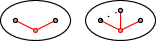
Figure 1: The planar Henneberg steps; the bottom vertex is new.

Figure 2: The Desargues graph.

Figure 3: All 1-skeleta of convex simplicial polyhedra on 6 vertices.

Figure 4: The spatial Henneberg steps. These are analyzed in Section 4.

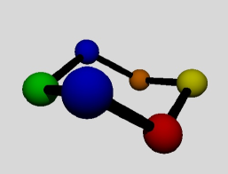
Figure 5: One of the spatial (chair) configurations of the cyclohexane molecule.

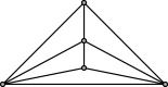
Figure 6: The only 1-skeleton of a simplicial polytope on 5 vertices.

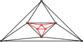
Figure 7: A Cyclohexane caterpillar with 2 copies.

References

- [1] C. Borcea. Point configurations and Cayley-Menger varieties, 2002. arXiv:math/0207110.
- [2] C. Borcea and I. Streinu. The number of embeddings of minimally rigid graphs. Discrete Comp. Geometry, 31(2):287–303, 2004.
- [3] R. Bowen and S. Fisk. Generation of triangulations of the sphere. Mathematics of Computation, 21(98):250–252, 1967.
- [4] D.N.Bernstein. The number of roots of a system of equations. Fun.Anal.Pril., 9:1–4, 1975.
- [5] I.Z. Emiris and J.F. Canny. Efficient incremental algorithms for the sparse resultant and the mixed volume. J. Symbolic Computation, 20(2):117–149, 1995.
- [6] I.Z. Emiris and B. Mourrain. Computer algebra methods for studying and computing molecular conformations. Algorithmica, Spec. Iss. Algor. Comp. Biology, 25:372–402, 1999.
- [7] I.Z. Emiris and A. Varvitsiotis. Counting the number of embeddings of minimally rigid graphs. In Euro. Workshop Comp. Geom., pages 151–154, Brussels, Belgium, 2009.
- [8] H. Gluck. Almost all simply connected closed surfaces are rigid. Lect. Notes in Math., 438:225–240, 1975.
- [9] D. J. Jacobs, A. J. Rader, L. A. Kuhn, and M. F. Thorpe. Protein flexibility predictions using graph theory. Proteins: Structure, Function, and Genetics, 44(2):150–165, 2001.
- [10] R. Steffens and T. Theobald. Mixed volume techniques for embeddings of Laman graphs. In Euro. Workshop Comp. Geom., pages 25–28, Nancy, France, 2008. Final version accepted in Comp. Geom: Theory & Appl., Spec. Issue.
- [11] M.F. Thorpe and P.M. Duxbury, editors. Rigidity theory and applications. Fund. Materials Res. Ser. Kluwer, 1999.
- [12] D. Walter and M. Husty. On a 9-bar linkage, its possible configurations and conditions for paradoxical mobility. In IFToMM World Congress, Besançon, France, 2007.
- [13] D. Walter and M. L. Husty. A spatial 9-bar linkage, possible configurations and conditions for paradoxical mobility. In NaCoMM, pages 195–208, Bangalore, India, 2007.
- [14] W. Wunderlich. Gefärlice annahmen der trilateration und bewegliche fachwerke i. Zeitschrift für Angewandte Mathematik und Mechanik, (57):297–304, 1977.