On the Implementation of the $0$–$1$ Test for Chaos

Abstract

In this paper we address practical aspects of the implementation of the $0$-$1$ test for chaos in deterministic systems. In addition, we present a new formulation of the test which significantly increases its sensitivity. The test can be viewed as a method to distill a binary quantity from the power spectrum. The implementation is guided by recent results from the theoretical justification of the test as well as by exploring better statistical methods to determine the binary quantities. We give several examples to illustrate the improvement.

1 Introduction

Being able to distinguish between regular and chaotic dynamics in a deterministic system is an important question with applications ranging from cardiac arrhythmias to the stability of our solar system. Much progress has been made in developing tests for chaos [13, 14, 25, 7, 2, 1]. Recently we have introduced a binary test for chaos, the $0$–$1$ test, designed for the analysis of deterministic dynamical systems [8, 9]. The test distinguishes between regular and chaotic dynamics for a deterministic system. The nature of the dynamical system is irrelevant for the implementation of the test; it is applicable to data generated from maps, ordinary differential equations and partial differential equations. The test has been applied to noisy numerical data [9], experimental data [5], quasiperiodically forced systems and strange nonchaotic attractors [3], Hamiltonian systems [26], nonsmooth systems [15] and fluid dynamics [18].

The usual test of whether a deterministic dynamical system is chaotic or nonchaotic involves the calculation of the maximal Lyapunov exponent $\lambda$ [13]. A positive maximal Lyapunov exponent indicates chaos: if $\lambda>0$, then nearby trajectories separate exponentially and if $\lambda\leq 0$, then nearby trajectories remain in a close neighbourhood of each other. This approach has been widely used for dynamical systems whose equations are known. If the equations are not known or one wishes to examine experimental data, then $\lambda$ may be estimated using the phase space reconstruction method of Takens [27], by approximating the linearisation of the evolution operator [24], or by the “direct method” [23].

In contrast our test does not depend on phase space reconstruction but rather works directly with the time series given. The main advantages of our test are (i) it is binary (minimizing issues of distinguishing small positive numbers from zero), (ii) the nature of the vector field as well as its dimensionality does not pose practical limitations, and (iii) it does not suffer from the difficulties associated with phase space reconstruction [13].

In this paper, we describe in detail how to implement the $0$–$1$ test for chaos. In addition, we carry out modifications to the test that greatly improve the previous versions in [8, 9].

Throughout the paper, we use the logistic map to illustrate our claims, with the exception of Section 6 where we use the Lorenz attractor as an example of a continuous time system. The reader can verify that our results apply equally well to other systems, including those considered in our previous papers [8, 9].

1.1 Recipe for the $0$–$1$ test

We briefly review how the test is implemented. Given an observation $\phi(j)$ for $j=1,\ldots,N$ we perform the following sequence of steps:

1. For $c\in(0,\pi)$, we compute the translation variables

   $$p_{c}(n)=\sum_{j=1}^{n}\phi(j)\cos jc,\quad q_{c}(n)=\sum_{j=1}^{n}\phi(j)\sin jc$$ (1.1)

   for $n=1,2,\ldots,N$. Typical plots of $p$ and $q$ for regular and chaotic dynamics are given in Fig. 1.

     

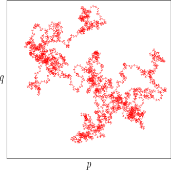
   Figure 1: Plot of $p$ versus $q$ for the logistic map $x_{n+1}=\mu x_{n}(1-x_{n})$. Left: Regular dynamics at $\mu=3.55$; Right: Chaotic dynamics at $\mu=3.9$. We used $5000$ data points.

2. The diffusive (or non-diffusive) behaviour of $p_{c}$ and $q_{c}$ can be investigated by analyzing the mean square displacement $M_{c}(n)$. The theory behind our test assures that if the dynamics is regular then the mean square displacement is a bounded function in time, whereas if the dynamics is chaotic then the mean square displacement scales linearly with time. In Section 2 we look at expressions for the mean square displacement and describe how one may use analytical expressions derived in [11] to conveniently modify the expression for the mean square displacement.

3. We then compute the asymptotic growth rate $K_{c}$ of the mean square displacement. Methods for the most effective estimation of this are discussed in Section 3.

4. Steps 1–3 are performed for $N_{c}$ values of $c$ chosen randomly in the interval $(0,\pi)$. In practice, $N_{c}=100$ is sufficient. The choice of $c$ is discussed further in Section 4. We then compute the median of these $N_{c}$ values of $K_{c}$ to compute the final result $K={\rm{median}}(K_{c})$. Our test states that a value of $K\approx 0$ indicates regular dynamics, and $K\approx 1$ indicates chaotic dynamics.

In this paper, we explore practical issues arising in the implementation of the above algorithm. Various issues associated with steps 2–4 are discussed in Sections 2–4 respectively. In Section 5 we examine finite data size effects. In particular we look at weak chaos. In Section 6 we consider continuous time systems where oversampled data can lead to small values of $K$ despite an underlying chaotic dynamics. In Section 7 we investigate the issue of measurement noise.

Remark 1.1

In the first version of our test, introduced in [8], we defined $p_{c}(n)$ and $q_{c}(n)$ by iterating the extended system

$$p_{c}(n+1) =p_{c}(n)+\phi(n)\cos(\vartheta_{c}(n))$$

$$q_{c}(n+1) =q_{c}(n)+\phi(n)\sin(\vartheta_{c}(n))$$

$$\vartheta_{c}(n+1) =\vartheta_{c}(n)+c+\alpha\,\phi(n)\;.$$

The current version of the test corresponds to the case $\alpha=0$. As shown in [9], the test with $\alpha=0$ is less sensitive to measurement noise.

Remark 1.2

It can be rigorously shown that (i) $p_{c}(n)$ and $q_{c}(n)$ are bounded if the underlying dynamics is regular, i.e. periodic or quasiperiodic and (ii) $p_{c}(n)$ and $q_{c}(n)$ behave asymptotically like Brownian motion for large classes of chaotic dynamical systems.

In [8] we used results of [6, 20, 21] to prove this for the case $\alpha\neq 0$ in Remark 1.1. In the case $\alpha=0$ these results are not applicable; nevertheless in [11] we cover the case $\alpha=0$ under even weaker assumptions on the underlying dynamics.

Remark 1.3

In [8, 11] it was shown that the results are valid for almost all observables $\phi$. Of course, the choice of the observable $\phi$ influences the rate of convergence (but not the limiting value $K=0$ or $K=1$). From a practical point of view we found that changing the observable does not greatly alter the computed value of $K$.

2 Computation of the mean square displacement

For a given time series $\phi(j)$ with $j=1,\ldots,N$, we compute the mean square displacement of the translation variables $p_{c}(n)$ and $q_{c}(n)$ defined in (1.1) for several values of $c\in(0,\pi)$. The mean square displacement is defined as

$$M_{c}(n)=\lim_{N\to\infty}\frac{1}{N}\sum_{j=1}^{N}[p_{c}(j+n)-p_{c}(j)]^{2}\,+\,[q_{c}(j+n)-q_{c}(j)]^{2}\;.$$ (2.1)

Note that this definition requires $n\ll N$. In [9] we calculated the mean square displacement using directly the definition (2.1). The limit is assured by calculating $M_{c}(n)$ only for $n\leq n_{\rm{cut}}$ where $n_{\rm{cut}}\ll N$. In practice we find that $n_{\rm{cut}}=N/10$ yields good results.

The test for chaos is based on the growth rate of $M_{c}(n)$ as a function of $n$. In the following, we use analytical expressions derived in [11] to formulate a modified mean square displacement $D_{c}(n)$ which exhibits the same asymptotic growth as $M_{c}(n)$ but with better convergence properties.

Under mild assumptions on the underlying dynamical system, described in Remark 2.1 below, for each $c\in(0,\pi)$,

$$M_{c}(n)=V\!(c)\,n+V_{\rm{osc}}(c,n)+e(c,n)\;,$$ (2.2)

where $e(c,n)/n\to 0$ as $n\to\infty$ uniformly in $c\in(0,\pi)$ and

$$V_{\rm{osc}}(c,n)=(E\phi)^{2}\frac{1-\cos nc}{1-\cos c}\;.$$

The expectation $E\phi$ is given by

$$E\phi=\lim_{N\to\infty}\frac{1}{N}\sum_{j=1}^{N}\phi(j)\;.$$

The form (2.2) suggests an improvement for the test: We can subtract the explicit term $V_{\rm{osc}}(c,n)$ from the mean square displacement and introduce

$$D_{c}(n)=M_{c}(n)-V_{\rm{osc}}(c,n)\;.$$ (2.3)

Note that the asymptotic growth rates of $M_{c}(n)$ and $D_{c}(n)$ are the same.

Figure 2: Plot of mean square displacement versus $n$ for the logistic map with $\mu=3.91$ corresponding to chaotic dynamics. The oscillating (green) curve is the original mean square displacement $M_{c}(n)$ as defined in (2.1); the straighter (red) curve is the modified mean square displacement $D_{c}(n)$ as defined in (2.3). We used $2000$ data points and computed $M_{c}(n)$ and $D_{c}(n)$ for $n=1,\ldots,200$ and $c=1.0$.

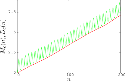
In Fig. 2 we show the two mean square displacements $M_{c}(n)$ and $D_{c}(n)$ for the logistic map $x_{n+1}=\mu x_{n}(1-x_{n})$ with $\mu=3.91$ (which corresponds to chaotic dynamics) and an arbitrary value of $c=1.0$. Evidently, the subtraction of the oscillatory term $V_{\rm{osc}}(c,n)$ regularizes the linear behaviour of $M_{c}(n)$. This allows a much better determination of the asymptotic growth rate $K_{c}$.

Remark 2.1

The autocorrelation function for the observation $\phi(j)$ is given by

$$\rho(k)=E(\phi(1)\phi(k+1))-(E\phi)^{2},\enspace k=0,1,2\ldots$$

Provided the autocorrelations are absolutely summable (that is, $\sum_{k=0}^{\infty}|\rho(k)|<\infty$) then equation (2.2) is valid, and moreover, the error term $e(c,n)$ decays uniformly in $c\in(0,\pi)$ (see for example [11]). It is for this reason that the test based on $D_{c}(n)$ greatly outperforms the test based on $M_{c}(n)$.

Furthermore, the absolute summability condition guarantees [11] that

$$V(c)=\sum_{k=-\infty}^{\infty}e^{ikc}\rho(|k|)=\lim_{n\to\infty}\frac{1}{n}E\Bigl{|}\sum_{j=0}^{n-1}e^{ijc}\phi(j)\Bigr{|}^{2}$$ (2.4)

for all $c\in(0,2\pi)$. This result follows from the Birkhoff ergodic theorem, the Wiener-Khintchine theorem, and standard calculations. In particular, the slope $V(c)$ of the mean square displacement is identified with the power spectrum.

For nonmixing systems, the error term $e(c,n)$ no longer decays to zero and there are further oscillatory terms in addition to $V_{\rm{osc}}(c,n)$. Nevertheless, the identification (2.4) remains valid for nonmixing systems under very weak conditions [19].

More importantly from the point of view of the test for chaos, working with $D_{c}(n)$ remains highly advantageous even for nonmixing systems. This is illustrated for the logistic map in Fig. 4 later in this paper,

3 Computation of $K_{c}$

Having calculated the modified mean square displacement $D_{c}(n)$ for $n=1,2,\ldots,n_{\rm{cut}}$, the next step is to estimate the asymptotic growth rate $K_{c}$. We have tried out two different methods: a regression method and a correlation method, described in subsections 3.1 and 3.2 below.

3.1 Regression method

The regression method consists of linear regression for the log-log plot of the mean square displacement. In [9] we used the original mean square displacement $M_{c}(n)$, so the asymptotic growth rate $K_{c}$ is given by the definition

$$K_{c}=\lim_{n\to\infty}\frac{\log{M}_{c}(n)}{\log n}\;.$$

Numerically, $K_{c}$ is determined by fitting a straight line to the graph of $\log M_{c}(n)$ versus $\log n$ through minimizing the absolute deviation [22].

In Section 2, we demonstrated the superiority of the modified mean square displacement $D_{c}(n)$ when compared to $M_{c}(n)$, so it is natural to apply the regression method to $D_{c}(n)$. Whereas $M_{c}(n)$ is strictly positive, $D_{c}(n)$ may be negative due to the subtraction of the oscillatory term $V_{\rm{osc}}(c,n)$. Hence, we set

$$\tilde{D}_{c}(n)=D_{c}(n)-\min_{n=1,\dots,n_{\rm cut}}D_{c}(n)\;,$$

and obtain the asymptotic growth rate

$$K_{c}=\lim_{n\to\infty}\frac{\log\tilde{D}_{c}(n)}{\log n}\;.$$

Again, $K_{c}$ can be determined numerically by regression (minimizing the absolute deviation) for the graph of $\log\tilde{D}_{c}(n)$ versus $\log n$.

Figure 3: Plot of $\log\tilde{D}_{c}(n)$ as a function of $\log n$ for the logistic map at $\mu=3.62$. We used $N=2000$ and calculated the mean square displacement up to $n_{\rm{cut}}=N/10$.

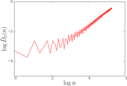
Remark 3.1

Minimizing the absolute deviation is preferable when compared to the usual least square method as the latter assigns a higher weight to outliers. Since the linear behaviour of the mean square displacement is only given asymptotically, one typically encounters outliers for small values of $n$. We find that it is usually sufficient to use the absolute deviation for estimating $K_{c}$, and that it is not necessary to employ more complicated higher-order regression methods such as the method by Yohai [17].

The finite value of the $o(n)$-term $e(c,n)$ in the definition of $M_{c}(n)$ in (2.2) leads to a distortion for small values of $n$. In such situations, one typically observes a flattening of the slope of $\log{M}_{c}(n)$ or $\log\tilde{D}_{c}(n)$ as illustrated in Fig. 3. It is those values for small $n$ of $\log{M}_{c}(n)$ (or $\log\tilde{D}_{c}(n)$) which would be overestimated in a least square fit.

3.2 Correlation method

We now present an alternative method for determining $K_{c}$ from the mean square displacement. (The method is described in terms of $D_{c}(n)$, but we could use $M_{c}(n)$ instead.)

Form the vectors $\xi=(1,2,\dots,n_{\rm cut})$ and $\Delta=(D_{c}(1),D_{c}(2),\dots,D_{c}(n_{\rm cut}))$. Given vectors $x$, $y$ of length $q$, we define covariance and variance in the usual way:

$${\rm cov}(x,y)=\frac{1}{q}\sum_{j=1}^{q}(x(j)-\bar{x})(y(j)-\bar{y}),\quad\text{where}\enspace\bar{x}=\frac{1}{q}\sum_{j=1}^{q}x(j)\;,$$

$${\rm var}(x)={\rm cov}(x,x)\;.$$

Now define the correlation coefficient

$$K_{c}={\rm corr}(\xi,\Delta)=\frac{{\rm{cov}}(\xi,\Delta)}{\sqrt{{\operatorname{var}(\xi)}{\operatorname{var}(\Delta)}}}\in[-1,1]\;.$$

This quantity measures the strength of the correlation of $D_{c}(n)$ with linear growth. Again, it can be shown rigorously [11] that under weak conditions on the underlying dynamics (as described in Remark 1.2) we obtain $K_{c}=0$ for regular dynamics and $K_{c}=1$ for chaotic dynamics.

Figure 4: Plot of $K$ versus $\mu$ for the logistic map with $3.5\leq\mu\leq 4$ increased in increments of $0.001$. We used $2000$ data points. The darker (red) lines are obtained by using the original definition of the mean square displacement $M_{c}(n)$ in (2.1). The lighter (green) lines are obtained by using the modified mean square displacement $D_{c}(n)$ in (2.3). The resulting values of $K$ are shown for the regression method (left) and the correlation method (right). The horizontal lines (blue and magenta) indicate the cases $K=0$ and $K=1$. We used $N_{c}=100$ values of $c$.

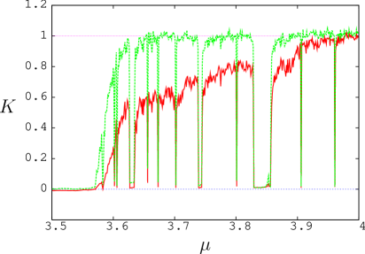
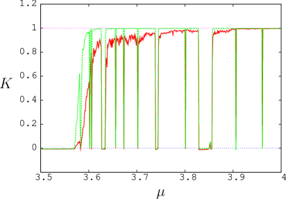
In practical terms, the correlation method greatly outperforms the regression method. This is evident from Fig. 4 which compares the regression method and the correlation method (using both $M_{c}(n)$ and $D_{c}(n)$) for the logistic map.

4 Choice of $c$ and determination of $K$

In Fig. 5 we show the asymptotic growth rate $K_{c}$ as a function of $c$ for regular and chaotic dynamics. In the case of periodic dynamics, most values of $c$ yield $K_{c}=0$ as expected, but there are isolated values of $c$ for which $K_{c}$ is large. (For the regression method, $K_{c}\approx 2$ at these resonant points.) These resonances are easily explained as follows: Equation (1.1) shows that if the Fourier decomposition of the observation $\phi$ contains a term proportional to $\exp(-i\omega k)$, then there is a resonance at $c=\omega$ where $p_{c}(n)\sim n$, and hence $M_{c}(n)\sim n^{2}$, irrespective of whether the dynamics is regular or chaotic. For the plots in Fig. 5, we have calculated the asymptotic growth rate using both the regression method described in Section 3.1 and the correlation method described in Section 3.2.

Figure 5: Plot of $K_{c}$ versus $c$ for the logistic map calculated using the regression method (top) and correlation method (bottom). We used here $N=5000$ data points, and $1000$ equally spaced values for $c$. Left: $\mu=3.55$ corresponding to regular dynamics; Middle: $\mu=3.9$ corresponding to chaotic dynamics; Right: $\mu=3.6$ corresponding to chaotic but non-mixing dynamics.

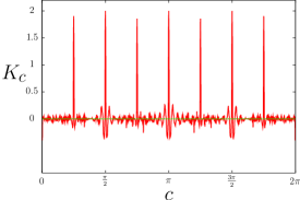
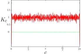
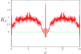
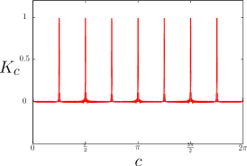
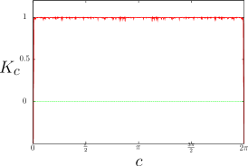
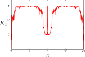
The occurrence of resonances for isolated values of $c$ suggests using the median of the computed values of $K_{c}$. (We use the median rather than the mean, since the median is robust against outliers associated with resonances.)

In Fig. 5c, $K_{c}$ is shown as a function of $c$ for $\mu=3.6$ where the dynamics is chaotic but not mixing on the whole interval $[0,1]$. The actual dynamics in the logistic map oscillates between two disjoint sets, each of which is mixing, and there is a resonance at $c=\pi$. At resonance, $p_{c}(n)\sim n$ and $M_{c}(n)\sim n^{2}$ as before. Close to resonance, the $p$-$q$ plot eventually behaves like Brownian motion, but in practice one sees only a small part of this motion and so $K_{c}\approx 0$.

Remark 4.1

Naturally, the choices of $c$ are equally spaced in Fig. 5, whereas in applying the test (and throughout the paper with the exception of Fig. 5) we choose randomly sampled values of $c$.

To avoid that resonances distort the statistics, we further restrict the range of randomly sampled values for $c$ to $c\in(\pi/5,4\pi/5)$ for all our computations. The resonance at $c=0$ is inherent to our test, but it may leak through adjacent values of $c$ as seen in Fig. 5c. The further restriction to exclude $\pi$ is not necessary, but we found it helpful. (A typical route to chaos is the Feigenbaum route via period doubling. Here, the parameter ranges for fixed points and period two points are largest.)

In Fig. 6, we show how the result for $K$ depends on the number $N_{c}$ of different values of $c$. Here we use the correlation version of the test to calculate $K_{c}$ as described in Section 3.2. There is no measurable gain in increasing $N_{c}$ from $100$ to $1000$ and we find that generally $N_{c}=100$ different values of $c$ is sufficient.

$\begin{array}[]{cc}\includegraphics[width=214.63977pt]{Fig6a_N.eps}&\includegraphics[width=214.63977pt]{Fig6b_N.eps}\\ \includegraphics[width=214.63977pt]{Fig6c_N.eps}&\includegraphics[width=214.63977pt]{Fig6d_N.eps}\\ \end{array}$

Figure 6: Plot of $K$ versus $\mu$ for the logistic map using the correlation method, with $3.5\leq\mu\leq 4$ increased in increments of $0.001$. We used $2000$ data points. Upper left: $N_{c}=1$; Upper right: $N_{c}=10$; Lower left: $N_{c}=100$; Lower right: $N_{c}=1000$.

5 Finite size problems

There are three types of finite size effects. First, the time series needs to be long enough to explore and sample the relevant phase space area (i.e. the attractor). This is an inherent problem affecting all tests for chaos. Second, the definition of the mean square displacement involves a limit which requires $n\ll N$. Accordingly, we have chosen $n\leq n_{\rm{cut}}=N/10$.

Third, the theory developed in [8, 11] makes statements about the asymptotic behaviour of $D_{c}(n)$ (or $M_{c}(n)$) and as such requires $n_{\rm cut}$, and hence $N$, to be sufficiently large. Finite size effect in this context means that for small $n$ the asymptotic linear growth is not yet dominating, see Fig. 3. This finite size effect is explored in the remainder of this section. From now on, we work exclusively with the modified mean square displacement $D_{c}(n)$ and the correlation method.

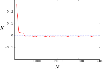
In Fig. 7 we show how the value of $K$ depends on the amount of data used. We can see clearly the convergence towards the asymptotic values $K=0$ and $K=1$ for regular and chaotic underlying dynamics, respectively. (For values of $\mu$ corresponding to stronger chaotic dynamics well within the chaotic range, the convergence towards $K=1$ is even more rapid.)

Figure 7: Plot of $K$ versus the available amount of data $N$ for the logistic map. Left: $\mu=3.55$ corresponding to regular dynamics; Right: $\mu=3.6$ corresponding to chaotic dynamics.

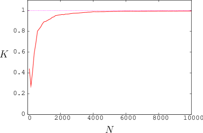
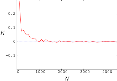
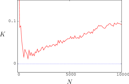
In the case of “weak chaos”, close to the so called “edge of chaos”, longer data sets are required to obtain $K=1$. Weak chaos is characterized by a slow decay of correlations. This has consequences for the modified mean square displacement $D_{c}(n)=V(c)n+o(n)$. For systems whose auto-correlation function is slowly decaying, it may be the case that the $o(n)$ term dominates for the available data. We illustrate this problem in the context of the logistic map. The bifurcation parameter $\mu$ takes the value $\mu=\mu_{\infty}=3.569945672\dots$ at the edge of chaos and for $\mu=\mu_{\infty}+0.001$ one observes weak chaos.

It has been erroneously claimed that our test cannot detect weak chaos, see [12, 10]. In fact, there are two methods whereby we can distinguish between regular dynamics and weak chaos:

• By visual inspection of the plot in the $p$-$q$ plane generated as in Fig. 8. (Note that for longer data sets the dynamics in the $p$-$q$ plane in Fig. 8b would look just like Fig. 1b.)

• By looking at the dependence of $K$ as a function of $N$. As illustrated in Fig. 9, we can distinguish weakly chaotic from regular dynamics even when the value of $K$ is very small – note that $K=0.027$ for $N=2000$ in the weakly chaotic case.

  

Figure 8: Plot of $p$ versus $q$ for the logistic map. Left: $\mu=\mu_{\infty}$; Right: $\mu=\mu_{\infty}+0.001$. We used $5000$ data points.

Figure 9: Plot of $K$ as a function of $N$ for the logistic map at $\mu=\mu_{\infty}$ (left) and $\mu=\mu_{\infty}+0.001$ (right). Although the value of $K$ is small in both cases, the behaviour of $K$ as a function of $N$ distinguishes the two cases.

6 Continuous time systems

In the previous sections, the $0$–$1$ test was formulated for discrete time systems. For continuous time series $\phi(t)$, there is a well-known oversampling issue that must be addressed. In this section, we discuss this difficulty and how to overcome it.

Given $0<t_{1}<t_{2}<t_{3}<\cdots$ we obtain a discrete time series $\phi(t_{1})$, $\phi(t_{2})$, $\phi(t_{3}),\ldots$ to which the test for chaos may be applied as in previous sections. (The sequence $t_{j}$, $j\geq 1$, should be chosen in a deterministic manner so that the time series $\phi(t_{j})$ is deterministic.) One method of choosing the $t_{j}$ is as the intersection times with a cross-section, so the time series $\phi(t_{j})$ corresponds to observing a Poincaré map. In this situation, there are no issues with oversampling.

A second, perhaps more usual, approach is to take $t_{j}=j\tau_{s}$ where $\tau_{s}>0$ is the sampling time. The time series $\phi(t_{j})=\phi(j\tau_{s})$ corresponds to observing the “time-$\tau_{s}$” map associated with the underlying continuous time system. If $\tau_{s}$ is too small, then the system is oversampled and this often leads to incorrect results. To illustrate the issue of oversampling we study the $3$-dimensional Lorenz system

$$\dot{x} ={\textstyle 10}(y-x)$$

$$\dot{y} ={\textstyle 30}\,x-y-xz$$ (6.1)

$$\dot{z} =xy-{\textstyle\frac{8}{3}}z\;,$$

which exhibits robust chaos. We have integrated this system with a time step of $\Delta t=0.001$ and recorded $100,000$ data points (ie. $100$ time units).

Fig. 10 shows an oversampled and a sufficiently coarsely sampled observable for the Lorenz system (6.1). The finely sampled time series ($\tau_{s}=0.005$) yields $K\approx 0$ even for $N=100,000$ whereas the coarsely sampled data ($\tau_{s}=0.05$) yields $K\approx 1$ already for $N=5,000$.

Figure 10: Plot of the observable $\phi(t)=x(t)$ for the Lorenz system (6.1). The finely sampled data (red) are sampled at $\tau_{s}=0.005$ time units. The coarsely sampled data (green filled circles) are sampled at $\tau_{s}=0.05$ time units.

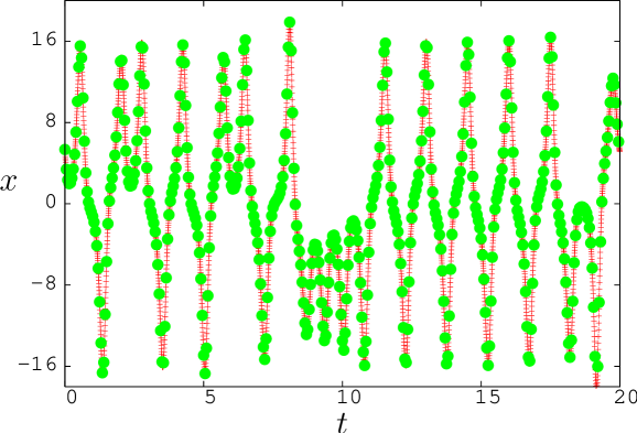
A good choice of the sampling time $\tau_{s}$ can often be obtained by visual inspection as in Fig. 10. A more refined method is to use the first minimum of the mutual information [4, 13]. For the data depicted in Fig. 10 this method yields $\tau_{s}=0.17$ (roughly a quarter of the oscillation period). Note however that in this particular instance the smaller sampling time $\tau_{s}=0.05$ already gives $K\approx 1$ and extracts a longer time series from the data in Fig. 10. In general, the optimal sampling time will depend on the dynamical system and the time series under consideration. We refer the reader to [13] for a discussion on optimal time delays in the context of phase space reconstruction.

Although oversampling is a practical problem for data series of finite size, it should be emphasized that theoretically the test works for all sampling times $\tau_{s}$ in the limit $N\to\infty$.

6.1 Oversampling and power spectra

For continuous time systems, the mean square displacement is defined as

$$M_{c}(t)=\lim_{T\to\infty}\frac{1}{T}\int_{0}^{T}(p_{c}(t+\tau)-p_{c}(\tau))^{2}\,+\,(q_{c}(t+\tau)-q_{c}(\tau))^{2}\;d\tau\;.$$

For a time series sampled with sample time $\tau_{s}$ this can be approximated by

$$M_{c}(n)=\lim_{N\to\infty}\frac{1}{N}\sum_{j=1}^{N}\left([p_{c\tau_{s}}(j+n)-p_{c\tau_{s}}(j)]^{2}\,+\,[q_{c\tau_{s}}(j+n)-q_{c\tau_{s}}(j)]^{2}\right)\tau_{s}^{2}\;.$$

Similarly the power spectrum for the time-continuous case discretizes to

$$S(\nu)=\lim_{n\to\infty}\frac{1}{n}E\Bigl{|}\sum_{j=0}^{n-1}e^{2\pi i\frac{\nu}{\nu_{s}}j}\phi(j)\Bigr{|}^{2}\tau_{s}^{2},$$ (6.2)

where $\nu_{s}=1/\tau_{s}$ is the sample frequency. The power spectrum consists of discrete peaks if the underlying system is regular, and is nowhere zero for a large class of chaotic systems [19]. However, for chaotic systems the power spectrum decays for large frequencies $\nu$, and so for frequencies larger than some $\nu_{\rm{max}}$ the power spectrum is zero for all practical purposes.

Comparing (6.2) with the power spectrum (2.4) for discrete-time data, we identify

$$c=2\pi\frac{\nu}{\nu_{s}},\quad\nu\in[0,\nu_{\rm{max}}]\;.$$

Sampling at the Nyquist rate with $\nu_{s}^{\star}=2\nu_{\rm{max}}$ yields $c\in(0,\pi)$ as before. However, oversampling at a higher frequency $\nu_{s}>\nu_{s}^{\star}$, restricts the effective choices of $c$ to $c\in(0,c^{\star})$ where $c^{\star}=\frac{\nu_{s}^{\star}}{\nu_{s}}\pi<\pi$. There is now a positive probability that the test for chaos will incorrectly yield $K=0$ since it is possible that more than half of the randomly chosen values of $c\in(0,\pi)$ will lie in $(c^{\star},\pi)$.

We illustrate the previous argument using the Lorenz system (6.1) sampled with $\tau_{s}$ ranging from $\tau_{s}=\Delta t$ up to $\tau_{s}=300\Delta t$. In Fig. 11 the median of the asymptotic growth rate $K$ is shown as a function of the sample time. For data that is too finely sampled, we obtain $K=0$ although the dynamics is actually chaotic.

Figure 11: Plot of $K$ as a function of the sample time $\tau_{s}$ for the Lorenz system (6.1). The sample time is measured in units of $\Delta t=0.001$.

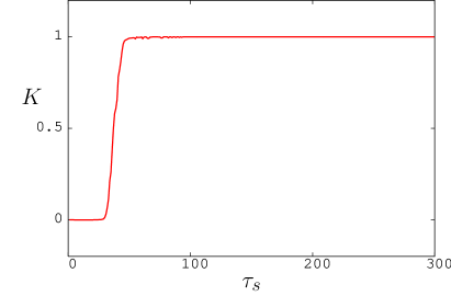
Fig. 12 illustrates how the range of effective values of $c$ depends on the sampling time $\tau_{s}$.

Figure 12: Plot of $K_{c}$ as a function of the frequency $c$ for the Lorenz system (6.1). From left to right we used $\tau_{s}=5\Delta t$, $\tau_{s}=10\Delta t$, $\tau_{s}=20\Delta t$, $\tau_{s}=30\Delta t$, $\tau_{s}=50\Delta t$, $\tau_{s}=70\Delta t$. The linear scaling of the range of $c$ for which $K_{c}\approx 1$ is evident in the relative spacing of the respective lines.

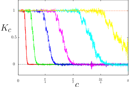
7 Noise contaminated data

Real-world data is invariably contaminated with noise. Any method for distinguishing regular from chaotic dynamics can only succeed if the noise-level is sufficiently small. There are various standard noise reduction techniques [13] that may be applied in advance of applying any given test for chaos. In addition, the test itself may be modified. Below we indicate a modification of the $0$–$1$ test for chaos that makes it more robust to the presence of noise.

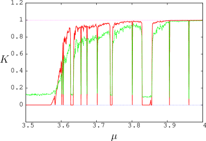
In [9] we introduced a version of the $0$–$1$ test that works well for data contaminated with measurement noise. (This is the test as presented in Sections 2 and 3, but using $M_{c}(n)$ instead of $D_{c}(n)$ and using the regression method instead of the correlation method.) We showed that the $0$–$1$ test clearly outperforms tangent space methods and compares favourably to “direct methods” based on phase space reconstruction. The improvements in this paper have made our test extremely sensitive to weak chaos. However, an unavoidable consequence is an increased sensitivity also to noise (see Fig. 13 below).

It turns out that the success of the version of the test in [9] is due to the oscillatory term $V_{\rm{osc}}(c,n)=(E\phi)^{2}\frac{1-\cos nc}{1-\cos c}$ that we subtracted in Section 2 to define the modified mean-square-displacement $D_{c}(n)=M_{c}(n)-V_{\rm{osc}}(c,n)$. This term desensitizes the test and damps the ability to detect slow growth of the mean-square-displacement for time-series data of moderate length. Instead of reintroducing this term we adopt a more flexible approach, defining

$$D^{\star}_{c}(n)=D_{c}(n)+\alpha V_{\rm damp}(n),\quad V_{\rm damp}(n)=(E\phi)^{2}\sin(\sqrt{2}n)\;.$$

(The frequency $\sqrt{2}$ was chosen arbitrarily.) For $\alpha$ large, we expect $K=0$. The amplitude $\alpha$ of the term $V_{\rm damp}(n)$ controls the sensitivity of the test to weak noise and simultaneously to weak chaos. This trade-off is unavoidable in any test for chaos.

As an illustration, we consider the logistic map with measurement noise. Take as observable $\phi(n)=x_{n}$ and write

$$\tilde{\phi}(n)=\phi(n)(1+\frac{\epsilon}{100}\eta_{n})$$

where $\eta_{n}$ are i.i.d. random variables drawn from a uniform distribution on $[-1,1]$ and $\epsilon$ is the noise-level in percent. Fig. 13 shows how the undamped version of the test in this paper copes with a noise level of $10\%$ and the improvement that is obtained by using the damped mean-square-displacement $D_{c}^{*}(n)$. We obtain similar results for normally distributed noise.

Figure 13: Plot of $K$ versus $\mu$ for the logistic map increased in increments of $0.001$. The darker (red) lines were computed using clean data. The lighter (green) lines were computed after addition of $10\%$ uniformly distributed measurement noise. Both lines were computed using the undamped mean-square-displacement $D_{c}(n)$. Left: $N=1000$ using the undamped mean-square-displacement $D_{c}(n)$, Right: $N=5000$ using $D_{c}(n)$. Bottom: $N=5000$ using the damped mean-square-displacement $D_{c}^{*}(n)$ with $\alpha=2.5$.

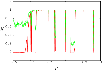
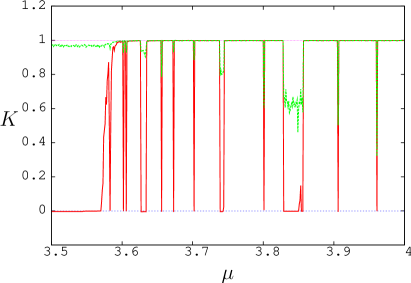
Remark 7.1

Under the assumption that the noise is diffusive and not correlated with the dynamics, the mean square displacement for data contaminated with measurement noise may be written as

$$D_{c}(n)=(V_{\rm{dyn}}(c)+V_{\rm{noise}}(c))n+o(n)\;,$$

where for a given value of $c$, $V_{\rm{dyn}}(c)$ is the variance associated with the deterministic dynamics and $V_{\rm{noise}}(c)$ the variance associated with the measurement noise. Consider an idealized situation where the value of $V_{\rm{noise}}(c)$ is roughly constant as a parameter $\lambda$ is varied. Suppose further that the dynamics is known to be regular at $\lambda=\lambda_{0}$. Then we may estimate $V_{\rm{noise}}(c)$ by making a gauge-measurement at $\lambda=\lambda_{0}$, applying the correlation method to $D_{c}(n)-Vn$. The unique value $V=V_{c}(\lambda_{0})$ which yields $K_{c}=0$ is our estimate for $V_{\rm{noise}}(c)$. For other values of $\lambda$ we may now apply the correlation method to $D_{c}(n)-V_{c}(\lambda_{0})n$.

8 Discussion

We have presented a guide for the implementation of the $0$–$1$ test for chaos. At the same time, we have introduced an improved version of the test which uses analytical expressions derived in [11]. Issues such as oversampling for continuous-time data and the presence of noise have been discussed. We hope that this guide will be helpful for scientists who would like to use the test.

There are numerous methods in the literature for distinguishing between deterministic and chaotic dynamics. In our previous papers [8, 9], we made a careful comparison of the $0$–$1$ test with methods for computing the maximal Lyapunov exponent. Another method is to use the power spectrum for which there are efficient computational techniques. It should be pointed out however that these techniques generally rely on the Wiener-Khintchine theorem which assumes summable decay of correlations and hence excludes periodic and quasiperiodic dynamics. Hence to use power spectra as a test for chaos, it seems necessary to avoid the Wiener-Khintchine theorem and to work directly with the expression $\lim_{n\to\infty}\frac{1}{n}E\Bigl{|}\sum_{j=0}^{n-1}e^{ijc}\phi(j)\Bigr{|}^{2}$. Equation (2.4) shows the relationship between the $0$–$1$ test and power spectra, and our test can be viewed as a way of condensing the information relevant for chaoticity or regularity contained in the power spectrum into a single binary number.

Acknowledgments

We would like to thank Ramon Xulvi-Brunet for pointing us towards the correlation method, and for explaining us the problem of oversampling in power spectra. We would like to thank Michael Breakspear and John Dawes for providing encouraging feedback on an earlier version of the manuscript. GAG is partly supported by ARC grant DP0452147 and DP0667065. The research of IM was partly supported by EPSRC grant EP/D055520/1 and by a Leverhulme Research Fellowship. IM is grateful to the University of Sydney for its hospitality.

References

- [1] R. Barrio. Sensitivity tools vs. Poincaré sections. Chaos Solitons & Fractals 25 (2005) 711–726.
- [2] P. M. Cincotta, C. M. Giordano and C. Simó. Phase space structure of multi-dimensional systems by means of the mean exponential growth factor of nearby orbits. Physica D 182 (2003) 151–178.
- [3] J. H. P. Dawes and M. C. Freeland. The ‘0–1 test for chaos’ and strange nonchaotic attractors. Preprint.
- [4] A. M. Fraser and H. L. Swinney. Independent coordinates for strange attractors from mutual information. Phys. Rev. A 33 (1986) 1134–1140.
- [5] I. Falconer, G. A. Gottwald, I. Melbourne and K. Wormnes. Application of the – Test for chaos to experimental data. SIAM J. Appl. Dyn. 6 (2007) 395–402.
- [6] M. Field, I. Melbourne and A. Török. Decay of correlations, central limit theorems and approximation by Brownian motion for compact Lie group extensions. Ergodic Theory Dyn. Syst. 23 (2003) 87–110.
- [7] M. Fouchard, E. Lega, C. Froeschlé and C. Froeschlé. On the relationship between fast Lyapunov indicator and periodic orbits for continuous flows. Celestial Mech. Dynam. Astronom. 83 (2002) 205–222.
- [8] G. A. Gottwald and I. Melbourne. A new test for chaos in deterministic systems. Proc. Roy. Soc. A 460 (2004) 603–611.
- [9] G. A. Gottwald and I. Melbourne. Testing for chaos in deterministic systems with noise. Physica D 212 (2005) 100–110.
- [10] G. A. Gottwald and I. Melbourne. Comment on “Reliability of the – test for chaos”. Phys. Rev. E 77 (2008) 028201.
- [11] G. A. Gottwald and I. Melbourne. Validity of the – test for chaos. In preparation.
- [12] J. Hu, W. -W. Tung, J. Gao and Y. Cao. Reliability of the – test for chaos. Phys. Rev. E 72 (2005) 056207.
- [13] H. Kantz and T. Schreiber. Nonlinear Time Series Analysis. Cambridge University Press, Cambridge, 1997.
- [14] J. Laskar. Frequency analysis for multi-dimensional systems. Global dynamics and diffusion. Physica D 67 (1993) 257–281.
- [15] G. Litak, A. Sytaa and M. Wiercigrochc. Identification of chaos in a cutting process by the – test. Chaos, Solitons & Fractals, in press.
- [16] E. Lorenz. Predictability - a problem solved,in Predictability (1996), edited by T. Palmer, European Centre for Medium-Range Weather Forecast, Shinfield Park, Reading, UK.
- [17] A. Marazzi, J. Joss and A. Randriamiharisoa. Algorithms, Routines, and S-Functions for Robust Statistics: The Fortran Library Robeth With an Interface to S-Plus. Chapman & Hall, 1993.
- [18] N. Martinsen-Burrell, K. Julien, M. R. Petersen and J. B. Weiss. Merger and alignment in a reduced model for three-dimensional quasigeostrophic ellipsoidal vortices. Phys. Fluids 18 (2006) 057101.
- [19] I. Melbourne and G. A. Gottwald. Power spectra for deterministic chaotic dynamical systems. Nonlinearity 21 (2008), 179–189.
- [20] I. Melbourne and M. Nicol. Statistical properties of endomorphisms and compact group extensions. J. London Math. Soc. 70 (2004) 427–446.
- [21] M. Nicol, I. Melbourne and P. Ashwin. Euclidean extensions of dynamical systems. Nonlinearity 14 (2001) 275–300.
- [22] W. H. Press, S. A. Teukolsky, W. T. Vetterling & B. P. Flannery. Numerical Recipes in C. Cambridge University Press, 1992.
- [23] M. T. Rosenstein, J. J. Collins and C. J. De Luca. A practical method for calculating largest Lyapunov exponents from small data sets. Physica D 65 (1993) 117–134.
- [24] M. Sano and Y. Sawada. Measurement of the Lyapunov spectrum from a chaotic time series. Phys. Rev. Lett 55 (1985) 1082–1085.
- [25] C. Skokos. Alignment indices: A new, simple method for determining the ordered or chaotic nature of orbits. J. Phys. A 34 (2001) 10029–10043.
- [26] C. Skokos, Ch. Antonopoulos, T. C. Bountis and M. N. Vrahatis. Detecting order and chaos in Hamiltonian systems by the SALI method J. Phys. A 37 92004) 6269–6284.
- [27] F. Takens. Detecting strange attractors in turbulence. Lecture Notes in Mathematics 98, Berlin: Springer, (1981) 366–381.
- [28] N. G. van Kampen. Stochastic Processes in Physics and Chemistry. North-Holland, Amsterdam, 2003.