Large scale bias and the inaccuracy of the peak-background split

Abstract

The peak-background split argument is commonly used to relate the abundance of dark matter halos to their spatial clustering.   Testing this argument requires an accurate determination of the halo mass function.  We present a Maximum Likelihood method for fitting parametric functional forms to halo abundances which differs from previous work because it does not require binned counts.   Our conclusions do not depend on whether we use our method or more conventional ones.  In addition, halo abundances depend on how halos are defined.  Our conclusions do not depend on the choice of link length associated with the friends-of-friends halo-finder, nor do they change if we identify halos using a spherical overdensity algorithm instead. The large scale halo bias measured from the matter-halo cross spectrum $b_{\times}$ and the halo autocorrelation function $b_{\xi}$ (on scales $k\sim 0.03h\,{\rm Mpc}^{-1}$ and $r\sim 50h^{-1}$Mpc) can differ by as much as 5% for halos that are significantly more massive than the characteristic mass $M_{*}$.   At these large masses, the peak background split estimate of the linear bias factor $b_{1}$ is 3-5% smaller than $b_{\xi}$, which is 5% smaller than $b_{\times}$. We discuss the origin of these discrepancies:  deterministic nonlinear local bias, with parameters determined by the peak-background split argument, is unable to account for the discrepancies we see.   A simple linear but nonlocal bias model, motivated by peaks theory, may also be difficult to reconcile with our measurements.  More work on such nonlocal bias models may be needed to understand the nature of halo bias at this level of precision.

1 Introduction

Halo abundances and clustering are both crucial ingredients in the halo model of large scale structure (Peacock & Smith, 2000; Seljak, 2000; Scoccimarro et al., 2001; Cooray & Sheth, 2002).   However, following Sheth & Tormen (1999), the two are not indepedendent:   an accurate model of halo clustering is part and parcel of an accurate model of halo abundances.  This is because of an argument that has come to be called the peak-background split (Bardeen et al., 1986; Cole & Kaiser, 1989; Mo & White, 1996), in which, on large scales, perturbed regions of the matter field are treated as though they are universes with slightly different mean density and Hubble constant (for an explicit calculation, see Martino & Sheth, 2009).

As a result, there has been considerable effort to provide simple, accurate and physically motivated functional forms for the halo mass function (Press & Schechter, 1974; Bond et al., 1991; Lee & Shandarin, 1998; Sheth et al., 2001), and to determine if such models provide adequate descriptions of the simulations.  When appropriately scaled, the functional form predicted by Press & Schechter (1974) is independent of power spectrum and cosmology.   Sheth & Tormen (1999) showed that, although this sort of rescaling of the mass function is not expected to hold exactly for the CDM family of models, it does produce an approximately universal curve in simulations, although the functional form of this universal curve is different from that of Press & Schechter (1974).  Subsequent work has confirmed that the mass function is indeed approximately universal (Jenkins et al., 2001; Reed et al., 2003), with only the most recent measurements beginning to detect the expected departures from universality (White, 2002; Reed et al., 2007; Tinker et al., 2008).   This is simply because the departures are small so large simulation volumes are required to see the effect with high significance.

The main goal of the present paper is to use the more precise measurements of halo abundances which can now be made (in simulations) to perform more precise tests of how well the peak background split argument works.  We do so by measuring halo abundances and clustering in large volumes, and then comparing the clustering signal with that predicted from the measured abundances by the peak background split ansatz.   We assess the robustness of our results by varying how we identify halos in the simulations; in each case, we use two different parametrizations for our measured abundances, and three different methods for fitting the parametrized models to the measurements.   We then compare the predicted and measured clustering signals in both real and Fourier space, and we do all this for two (and sometimes three) different redshifts.

At this level of precision, the comparison of measurement and prediction is somewhat subtle, because it depends on the details of whether or not the bias is expected to be deterministic or stochastic, local or nonlocal, linear or nonlinear, constant or scale-dependent.  We study two limiting cases in detail: a bias which is deterministic and local in configuration space, and is scale independent at linear order but contains higher order nonlinear terms, and a bias which is deterministic and linear in Fourier space, with no higher order terms, but the linear bias is $k$-dependent.  The former arises naturally in the simplest models of halo abundances; the latter is motivated by associating nonlinear stuctures with peaks in the initial density fluctuation field.

This paper is organized as follows: Section 2 gives some theoretical background and describes a number of ways one might have quantified the bias between the halo and matter distributions.  It then specifies the particular ways we have adopted for our test.   Section 3 presents measurements of halo abundances and clustering in our simulations, and comparison with the bias predicted by the peak background split argument.   A final section summarizes our results and conclusions. Appendix A describes a number of ways we have attempted to fit the halo mass function, one of which is a new Maximum Likelihood estimator of halo abundances that does not require binned counts. Appendix B provides explicit expressions for the peak background split bias factors associated with our parametrizations of the halo mass function.

2 Background

2.1 Counts in cells and the peak background split

The peak background split (Bardeen et al., 1986; Cole & Kaiser, 1989) is an approximation in which the effect of long wavelength density perturbations on structure formation is simply to modify the collapse times of non-linear objects.  This modification depends on the density of the perturbed region but not on its volume.  It is common to state that the number density of halos in a perturbed region is expected to be the same as that of an unperturbed region, but at a slightly different time.  However, it is better to think of the perturbed number density as being the same as that of an unperturbed region in a different background cosmology (after all the density is different), but one that has the same age (meaning the effective Hubble constant is different) (Martino & Sheth, 2009).  When expressed in terms of linear theory quantities, this effect changes the critical density for non-linear collapse in a way that depends on the nonlinear density of the perturbation (Mo & White, 1996).

Thus, while in general the mean number of halos of mass $m$ in a cell depends on its volume $V$ and mass $M$, in this approximation, for cells for cells which are sufficiently large that $m\ll M$, the overdensity of halos depends, not on $M$ and $V$, but on $M/V=1+\delta$.   That is to say,

$$\langle N_{\rm h}(m,\delta_{c}|M,V)\rangle\equiv n_{\rm h}(m,\delta_{c})V\,[1+\langle\delta_{h}(m|\delta)\rangle]$$ (1)

where $n(m,\delta_{c})$ is the average number density of halos with mass $m$, and

$$\langle\delta_{h}(m)|\delta\rangle=\sum_{k>0}\frac{b_{k}(m,\delta_{c})}{k!}\,             \Bigl{(}\delta^{k}-\langle\delta^{k}\rangle\Bigl{)}.$$ (2)

The coefficients $b_{k}(m,\delta_{c})$ come from Taylor expanding $n(m,\delta_{c}-\delta)$ around $\delta=0$, and the $\langle\delta^{k}\rangle$ terms are required if one wishes to truncate the expansion at finite $k$ but still enforce $\langle\delta_{h}(m)|\delta\rangle=0$.   Thus, in this framework, halo bias is deterministic ($\delta$ is the only random field that determines $\delta_{h}$) but nonlinear (high order terms in $\delta$ contribute), so it is of the form discussed by e.g. Fry & Gaztanaga (1993).

The most direct check of this assumption is to measure the quantity on the left hand side of equation (2) in large cells $V$, and compare with the coefficients one predicts from the mass function (Sheth & Lemson, 1999; Smith et al., 2008).  Note that this is explicitly a real-space, counts-in-cells calculation.   It is, however, a difficult approach, since the halo bias coefficients of interest are those for large cells, but these tend to have small variance (the universe is homogeneous on large scales), meaning that there is only a small range of $\delta$ over which to measure the shape of the halo bias relation.  In practice, measuring $b_{2}$ is tough, and $b_{3}$ is even more challenging.

2.2 Other measures of the linear bias factor

A less direct measure of this bias is given by the volume average of the cross correlation function between halos and mass.  In this case, one measures

$$1+\sigma^{2}_{\rm hm}(V) = \int dM\,p(M|V)\,\sum p(N_{h}|M,V)                          \frac{M}{\bar{\rho}V}\,\frac{N_{h}}{n_{\rm h}V}$$

$$= \int dM\,p(M|V)\,\frac{M}{\bar{\rho}V}\,              \frac{\langle N_{h}|M,V\rangle}{n_{\rm h}V}$$

$$= 1+\sum_{k>0}\frac{b_{k}}{k!}\langle\delta_{M}^{k+1}\rangle$$

$$= 1+b_{1}\sigma_{M}^{2}+\ldots$$ (3)

where $\sigma^{2}_{\rm hm}(V)$ is the cross-correlation between halo and mass counts in cells of size $V$, $p(M|V)$ is the probability a randomly chosen cell of size $V$ contains mass $M$, and

$$\sigma_{M}^{2}\equiv\langle\delta_{M}^{2}\rangle =\int\frac{dk}{k}\,\frac{k^{3}\,P(k)}{2\pi^{2}}\,W^{2}(kR)$$ (4)

where $P(k)$ is the power spectrum of the mass, and $W$ is the Fourier transform of the smoothing volume (so $V\propto R^{3}$).

And even more indirect is the second factorial moment of the halo counts-in-cells:

$$1+\sigma^{2}_{\rm hh}(V) = \int dM\,p(M|V)\,\sum p(N_{h}|M,V)                          \frac{N_{h}}{n_{\rm h}V}\frac{N_{h}-1}{n_{\rm h}V}$$

$$= \int dM\,p(M|V)\,           \frac{\langle N_{h}(N_{h}-1)|M,V\rangle}{(n_{\rm h}V)^{2}}.$$ (5)

If the halo counts in cells $(M,V)$ follow a Poisson distribution around the mean $\langle N_{h}|M,V\rangle$ (this is a bad assumption when $m$ is not small compared to $M$), then this becomes

$$1+\sigma^{2}_{\rm hh}(V) = \int dM\,p(M|V)\,           \frac{\langle N_{h}|M,V\rangle^{2}}{(n_{\rm h}V)^{2}}$$

$$= 1+b_{1}^{2}\sigma_{M}^{2}+\ldots$$ (6)

Finally, it is worth noting that

$$\sigma^{2}_{\rm hm}(R) = \int\frac{dk}{k}\,\frac{k^{3}P_{\rm hm}(k)}{2\pi^{2}}\,W^{2}(kR)$$ (7)

$$= 4\pi\int_{0}^{2R}drr^{2}\,\xi_{\rm hm}(r)\,            \frac{3}{\pi}\frac{(4+r/R)(2-r/R)^{2}}{32R^{3}}$$

where the final expression assumes tophat smoothing.   Similar relations hold for $\sigma_{\rm hh}$, $\xi_{\rm hh}$ and $P_{\rm hh}$.

So, if $b_{1}$ is independent of scale, then the slope of the regression of $\delta_{h}$ on $\delta_{m}$ is the same quantity as $\sigma_{\rm hm}^{2}/\sigma^{2}$ and $\xi_{\rm hm}/\xi$; and if the counts are Poisson, then this is also the same as $\sqrt{\sigma^{2}_{\rm hh}/\sigma^{2}}$, $\sqrt{\xi_{\rm hh}/\xi_{\rm dm}}$, $\sigma^{2}_{\rm hh}/\sigma^{2}_{\rm hm}$, and $\xi_{\rm hh}/\xi_{\rm hm}$ at large scales. In addition, if $b_{1}$ is independent of scale, then the bias in Fourier space quantities is simply related to (equal to!) those in configuration space.  In particular, $\sqrt{P_{\rm hh}(k)/P(k)}$, $P_{\rm hh}(k)/P_{\rm hm}(k)$ and $P_{\rm hm}(k)/P(k)$ should all equal $b_{1}$ at low k.   But in general, all these quantities are different.   We discuss some of the differences expected in concrete bias models and in view of our measurements below.

Even if these bias factors are equal, actually estimating $P_{\rm hh}$ is difficult because the measurement requires a shot-noise correction for the discreteness of the halos.  Because the massive halos of most interest in the present study are rare, this correction can be significant, but because they are strongly clustered, this correction is currently uncertain (Smith et al., 2008). There is no shot-noise correction for $P_{\rm hm}$, so, in what follows, this is the statistic we will use to test the peak background split expression for the linear bias parameter $b_{1}$.  We also test the ratio $\sqrt{\xi_{\rm hh}/\xi_{\rm dm}}$, for which no shot-noise correction is necessary.

2.3 The effects of nonlinearity on large-scale bias

Differences between the predicted $b_{1}$ and the large scale bias measured from correlation functions are expected if the bias is nonlinear.  Indeed, the peak-background split itself predicts that halo bias is not linear (the higher order coefficients in equation 2 are generically non-zero), and such nonlinearities are seen in numerical simulations (see, e.g., scatter plots of $\delta_{h}$ vs $\delta_{m}$ in Appendix B of Smith et al., 2007).   This complicates interpretation of the measured values of $P_{hm}/P_{mm}$ and $\sqrt{\xi_{\rm hh}/\xi_{\rm dm}}$ as follows.

In the local bias framework of equation (2), the halo-mass cross-correlation reads

$$\mathop{\langle}\delta_{h1}\delta_{2}\mathop{\rangle}= b_{1}\mathop{\langle}\delta_{1}\delta_{2}\mathop{\rangle}+{b_{2}\over 2}\mathop{\langle}\delta_{1}\delta_{2}^{2}\mathop{\rangle} +{b_{3}\over 6}\mathop{\langle}\delta_{1}\delta_{2}^{3}\mathop{\rangle}+\ldots$$ (8)

where 1 and 2 denote two different spatial positions.   In the large-scale limit, perturbation theory says that

$$\mathop{\langle}\delta_{1}^{p}\delta_{2}^{q}\mathop{\rangle_{c}}\equiv C_{pq}\,\sigma^{2(p+q-2)}_{R}\ \xi$$ (9)

where $\sigma^{2}_{R}$ denotes the variance in the dark matter field when smoothed on scale $R$, and $C_{pq}$ are closely related to the skewness, kurtosis and so on.  E.g., $C_{21}=68/21+\gamma_{R}/3$, with $\gamma_{R}\equiv d\ln\sigma^{2}_{R}/d\ln R$ and $C_{pq}=C_{p1}C_{q1}$ (Bernardeau, 1996; Gaztanaga et al., 2002).   Thus, on large scales, the cross-correlation bias is

$$b_{\times}\equiv{\mathop{\langle}\delta_{h1}\delta_{2}\mathop{\rangle}\over\xi}         =b_{1}+{\sigma^{2}_{R}\over 2}\Big{(}C_{21}\,b_{2}+b_{3}\Big{)}               +{\sigma^{4}_{R}\over 6}C_{31}\,b_{3}+\ldots,$$ (10)

and it applies equally well in configuration and Fourier space.   Keeping only the first order corrections to linear bias, yields

$$b_{\times}=\frac{P_{hm}(k|R)}{P(k)}         =b_{1}+\sigma_{R}^{2}\left[\Big{(}\frac{34}{21}+{\gamma_{R}\over 6}\Big{)}b_{2}+\frac{b_{3}}{2}\right]$$ (11)

for the Fourier-space quantity (e.g. Smith et al., 2007, who neglected the $\gamma_{R}$ term), where $P_{hm}(k|R)$ denotes the cross-power of the halo and mass fields when both have been smoothed with a filter of scale $R$.

In the present context, for halos of a given mass, the peak-background split argument gives the values of $b_{i}$.  However, the choice of smoothing scale $R$ is less straightforward.  It must be large enough that the assumptions of a deterministic, scale independent bias are reasonably accurate, so $R$ must be substantially larger than the Lagrangian radius of the halos (Sheth & Lemson, 1999; Smith et al., 2008; Manera & Gaztañaga, 2009).   But there is no other underlying theory for this scale.

The same logic that led to equation (10) says that

$$b^{2}_{\xi} =  \frac{\mathop{\langle}\delta_{h1}\delta_{h2}\mathop{\rangle}}{\xi}          =   b_{1}^{2}+b_{1}\,\sigma^{2}_{R}\,(C_{21}\,b_{2}+b_{3})                     + {b_{2}^{2}\over 2}\,\xi$$

$$\qquad\qquad\qquad+\sigma^{4}_{R}\,  \Big{(}{b_{1}b_{3}\over 3}\,C_{13}+{b_{2}^{2}\over 4}\,C_{22}\Big{)}+\ldots$$ (12)

$$\simeq b_{\times}^{2}-\sigma^{4}_{R}\,\frac{b_{3}}{4}         \left(b_{3}+2b_{2}C_{12}\right)\,+\frac{b_{2}^{2}}{2}\,\xi.$$

The final expression shows that $b_{\xi}\neq b_{\times}$ even when $\sigma^{2}_{R}\ll 1$.   And the $\xi$ term in $b_{\xi}$ generates a shot-noise contribution at low-$k$ in the power spectrum.

bias symbol	meaning	equation
$b_{1}$, $b_{2}$, $b_{3}$	First (linear), second and third order bias from                      Taylor expansion of the fluctuation in                      the mass density field.  This is a deterministic                      local bias model for which predictions exist                      from the peak background split argument in the                      large cell limit.	(2)
$b_{\times}$	Large scale bias from the matter-halo cross power.             Values taken at $k=0.03h$Mpc-1.	(11)
$b_{\xi}$	Large scale bias from the correlation function.          Values are taken by averaging $\xi$ over          $40\leq r\leq 60h^{-1}$Mpc.	(12)
$b_{\nu}$, $b_{\zeta}$	Linear and quadratic bias from the high peaks model.	(13)

Table 1: Notation for the various bias factors used in this paper.

2.4 The peaks-bias model

The previous discussion supposed that the fundamental quantity was the bias between halo and mass counts in cells.  An alternative model is that (high) peaks in the initial density field are the seeds around which massive halos form (Kaiser, 1984).   In this case the large scale bias is simplest in Fourier space:

$$\delta_{pk}(k)=(b_{\nu}+b_{\zeta}k^{2})\,W_{pk}(kR_{pk})\delta(k),$$ (13)

where $W_{pk}$ is the smoothing filter with which the peak was identified (Matsubara, 1999; Desjacques, 2008).

Typically, to approximate halos of mass $m$ by peaks, one uses a Gaussian smoothing filter with $m\propto R_{pk}^{3}$.  In this case, a halo of mass $m$ is associated with a peak of height $\nu=\delta_{pk}/\sigma_{0}$, where $\delta_{pk}$ is of order unity as suggested by the spherical evolution model, and $\sigma_{0}^{2}$ is given by equation (4) but with smoothing scale $R_{pk}$. At high masses, the resulting peak mass function is similar to that of halos (Sheth, 2001). The quantity $b_{\zeta}\propto(\sigma_{0}/\sigma_{1})^{2}\,(\nu/\sigma_{0}-b_{\nu})$, where $\sigma_{1}^{2}$ is similar to $\sigma_{0}^{2}$, but with an extra factor of $k^{2}$ in the integral in equation (4). For a power law power spectrum with $P(k)\propto k^{n}$, $(\sigma_{0}/\sigma_{1})^{2}\propto m^{2/3}$.  In the high peak ($\nu\gg 1$) limit, $b_{\nu}\to(\nu-3/\nu)/\sigma_{0}$ so $\nu/\sigma_{0}-b_{\nu}\to 3/(\sigma_{0}\nu)$.   In this limit, $b_{\zeta}$ increases as $m$ increases, and $(b_{\zeta}/b_{\nu})\to(\sigma_{0}/\sigma_{1})^{2}(3/\nu^{2})                \propto m^{2/3-(n+3)/3}$, a point to which we will return later.

Equation (13) implies that

$$P_{pk,\delta}(k) = (b_{\nu}+b_{\zeta}k^{2})\,W_{pk}(kR_{pk})\,P_{\rm L}(k),$$ (14)

$$P_{pk,pk}(k) = (b_{\nu}+b_{\zeta}k^{2})^{2}\,W^{2}_{pk}(kR_{pk})\,P_{\rm L}(k),$$ (15)

so $P_{pk,\delta}(k)/P(k)$, $\sqrt{P_{pk,pk}(k)/P(k)}$ and $P_{pk,pk}(k)/P_{pk,\delta}(k)$ all measure the same quantity (even though the quantity depends on $k$!), but the bias relations from correlation functions or counts in cells will be more complicated (because of the $k$ dependence).  In particular, notice that, in contrast to the previous model, here the linear bias factor itself is scale-dependent.

Now, the bias relations above are for peaks identified in the initial fluctuation field. At this time $b_{1}$ from the peak background split calculation equals $b_{\nu}$ from the Fourier bias calculation (Desjacques & Sheth, 2009).   (In principle, at least for peaks, this agreement can be used as a guide to the appropriate shot-noise correction for $P_{pk,pk}(k)$ – like massive halos, high peaks are rare, so the shot-noise correction matters – but this is beyond the scope of this paper.) A peak background split estimate for the late time bias parameters $b_{1}$, $b_{2}$, etc. of peaks was made by Mo et al. (1997).  This estimate says that $b_{1}\to 1+b_{1}$ (with similar consequences for $b_{2}$ etc.), and is in reasonable agreement with measurements in simulations of $\sqrt{\sigma^{2}_{pk,pk}/\sigma^{2}}$ and $\sqrt{\xi_{pk,pk}/\xi}$ (Mo et al., 1997) (i.e., within the accuracy of what was possible with the smaller simulation volumes of 10 years ago).   This suggests that $b_{\nu}$ evolves as $b_{1}$, but a good model for the evolution of $b_{\zeta}$ is still not available. Therefore, when we compare the peaks model with measurements in simultions, we will simply consider if a $k^{2}$ scaling of the bias factor seems appropriate, and if the onset of this term occurs at smaller $k$ for halos of higher masses.

3 Measurements in simulations

3.1 Description of the simulations

For our analysis we use 49 cosmological dark matter simulations of a flat $\Lambda$CDM cosmology with $\Omega_{m}=0.27$, $\Omega_{\Lambda}=0.73$, $\Omega_{b}=0.046$, $\sigma_{8}=0.9$, $h=0.72$  and $n_{s}=1.0$.   Each simulation was run using periodic boundary conditions in a box of size $L_{box}=1280h^{-1}$Mpc, which contains $640^{3}$ particles. This gives a particle mass of $M_{p}\simeq 6\times 10^{11}h^{-1}M_{\odot}$. All 49 runs have the same parameters except for the random seeds used to generate the initical conditions. Therefore they can be considered as different realizations (or parts) of the same universe; this allows us to estimate errors on the mass function and bias factors we measure in the next section.   For reference, the total volume sampled by our runs is $V_{\rm T}\simeq 102h^{-3}$  Gpc³.

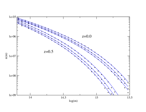
Figure 1: Mass function at $z=0$ (upper set of curves) and $z=0.5$ (lower set of curves) for three linking lengths in simulations: 0.15 (fewest massive halos), 0.168 and 0.2 (most massive halos). Lines show equation (19) with parameters from our new Maximum Likelihood estimator (see Table 2).

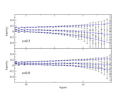
Figure 2: Same as figure 1, only now, to better see  the range on the plot, the mass functions have been divided  by a fiducial function (equation 19 with $p=0.33$ and $q=0.75$). Error bars show the rms variation between simulations.

One potentially important difference from almost all previous work in which volumes of this size have been studied is in how we generate our initial conditions.  These are set at $z=50$ by using CMBFAST (Seljak & Zaldarriaga, 1996) to generate the Transfer function for the initial matter power spectrum.  We then use a Second Order Lagrangian Perturbation Theory (2LPT) code (Scoccimarro, 1998) to generate the initial displacement field.   The use of 2LPT initial conditions ensures that spurious transient effects in the simulations are negligible at low redshifts (Crocce et al., 2006). The tree-PM code Gadget-2 (Springel, 2005), with a softening length set to 20$h^{-1}$kpc, is then used to simulate the subsequent evolution.

3.2 The halo mass function

We have run a standard friends-of-friends (FoF) code to identify dark matter halos in the simulations at redshifts $z=0$ and $z=0.5$. The halo mass function one obtains depends on the one free parameter of the FOF algorithm:  the linking length. Shorter linking lengths return lower mass halos.   Since halo abundances and clustering strength are intimately related, the choice of linking length also affects the halo bias parameters. To address this, we have explored three choices: $l_{\rm link}=0.15,0.168$ and 0.2 (in units of the interparticle separation).

The halo mass of each object found by the FoF algorithm was determined from the number of particles $N$ it contains, corrected for discreteness effects following Warren et al. (2006). Thus, $M_{h}=M_{p}N_{\rm corrected}$, where $N_{\rm corrected}=N(1-N^{-0.6})$.   This correction has been tested only for FoF halos with $l_{link}=0.2$, and may sligtly overcorrect the mass for smaller linking lengths. Since in this paper we are fitting the mass function for halos having more than 105 particles, these differences are negligible for the large mass halos which are of most interest in what follows.

It is common to use the same linking length for all redshifts.   However, the natural outcome of the spherical collapse model predicts that, in $\Lambda$CDM models, halos are a larger multiple of the background density at late times.   If this model is correct, then one expects the appropriate link length to be approximately constant at early times, and to decrease at late times.  Our choices of linking-length approximately bracket the expected range of densities.

Another popular choice for identifying halos is to require them to be a fixed multiple of the critical density. In $\Lambda$CDM models, this has the virtue of being well-motivated at early times (when the background cosmology is effectively Einstein-de Sitter, so the background and critical densities are equal) as well as at very late times (when the critical density has become constant).   In section 3.8 we use halos identified using a spherical overdensity method by Tinker et al. (2008).  However, in this case, the overdensity was a fixed multiple (200) of the background density.   We find that the main results which follow are robust to which halo finder we use.

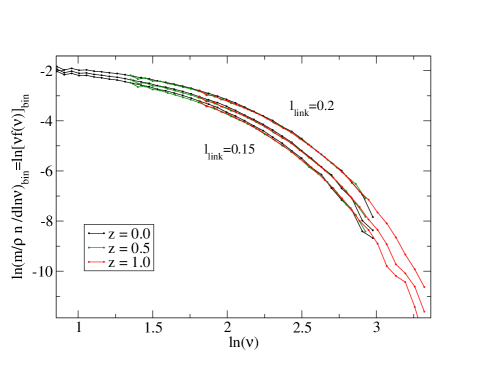
Figure 3: Same as Figure 1, but now shown in scaled units, so outputs from $z=0,0.5$ and $1$ are shown together.   Because we only count halos with more than 105 particles, the lower redshift output probes to smaller $\nu$, and the higher redshift output to higher $\nu$. Results for the three linking lengths are shown: 0.15, 0.168 and 0.2. For a fixed $\nu$ larger $l_{\rm link}$ yields more halos.

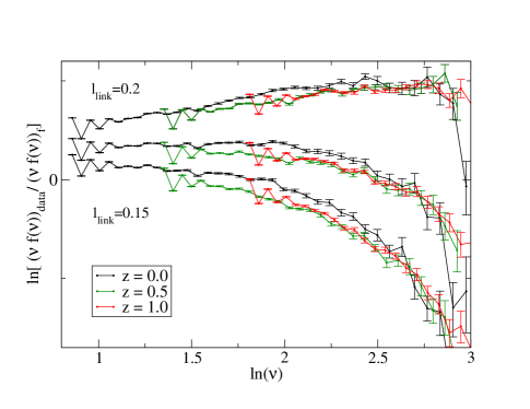
Figure 4: Same as Figure 2, but now in scaled units. Error bars show the error on the mean value between simulations.

Figure 1 shows the mass functions associated with the three linking lengths at $z=0$ and $z=0.5$.   To emphasize detailed differences, we show this same information divided by a fiducial model for halo abundances in Figure 2. The fiducial model is that of equation (19) below, with $p=0.75$ and $q=0.33$.   In these, as in all the plots to follow, the bins are 0.05 dex in mass, and error bars, unless stated otherwise, show the rms variation between simulations.   The true error on the mean is a factor of $\sqrt{49}=7$ smaller. It is interesting to ask if the halo catalog returned by a shorter link-length is essentially a higher redshift version of the halo catalog associated with the longer link-length.  We will have more to say about this shortly, but note that this dependence on linking length is not naturally included in models of halo abundances (e.g. Sheth et al., 2001).

When the masses are suitably rescaled, the mass function can be expressed in a functional form that is nearly universal - being approximately independent of time, cosmology, and initial power spectrum (Sheth & Tormen, 1999).  The spherical evolution model suggests that the natural scaling variable should be

$$\nu\equiv\frac{\delta^{2}_{\rm sc}(\Omega_{z},\Lambda_{z})}{D^{2}(z)\,\sigma_{0}^{2}(m)}$$ (16)

where $\delta_{\rm sc}$ is the critical density required for spherical collapse in a cosmology with parameters $(\Omega_{z},\Lambda_{z})$, $D(z)$ is the linear theory growth factor in units of its value at $z=0$ [e.g. $D(z)=(1+z)^{-1}$ and $\delta_{\rm sc}(z)=1.686$ if $(\Omega_{z},\Lambda_{z})=(1,0)$], and

$$\sigma_{0}^{2}(m)=\int\frac{dk}{k}\,\frac{k^{3}\,P_{0}(k)}{2\pi^{2}}\,W^{2}(kR_{m})$$ (17)

with $m=\bar{\rho}\,(4\pi R_{m}^{3}/3)$ and $W(x)=(3/x^{3})\,(\sin x-x\cos x)$.  Here $P_{0}(k)$ denotes the initial power spectrum of fluctuations, scaled using linear theory to $z=0$, and $\bar{\rho}$ is the comoving background density.

So, one measure of the best link-length is to see which one provides the most universal scaling.  Figure 3 shows the mass functions in these scaled units, $\nu$, and Figure 4, shows these curves divided by the same fiducial model as before.  Because we only have a fixed mass range in the simulations, the higher redshift outputs mainly probe the $\nu\gg 1$ end of the mass function.  Therefore, in these figures, we also show results for $z=1$.

It is not obvious that any one link length produces more self-similar scalings than the others.  What is more apparent is that, whatever the link-length, the $z=0$ abundances appear to be offset to slightly larger values compared to those at higher $z$.   This is in qualitative agreement with the spherical model, which predicts that halos should be increasingly dense relative to the background at late times, meaning that the appropriate link length should be smaller at late times.  By using a fixed link length, we will overestimate halo masses, and hence the abundance at large $\nu$.

A slight variation on the appropriate self-similar scaling is to ignore the $z$ dependence of $\delta_{\rm sc}$.  Although this has no physical motivation, it is a popular choice   (e.g. Jenkins et al., 2001; Reed et al., 2003; Warren et al., 2006).  We have found that this makes the mass function slightly less universal (the offset at $z=0$ is slightly more pronounced), but since we are not scaling the link-lengths with time in the way the spherical model suggests, we do not think our measurements advocate strongly for including the $z$-dependence of $\delta_{\rm sc}$.

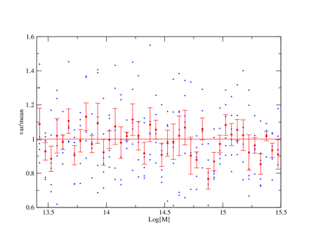
Figure 5: Ratio of variance of halo counts between runs to mean halo count for a number of bins in mass.   For each mass bin, error bars show the error on the mean between the six measurements of this ratio (the three link lengths at each of two redshift bins).  If the counts were Poisson, this ratio would be unity, with a typical spread of about $0.2$ (see text in section 3.6).  

Method:		New ML method		Poisson ML method		$\chi^{2}$ method		New ML method		Poisson ML method		$\chi^{2}$ method
z	$l_{\rm link}$	q	p	q	p	q	p	rms(q)	rms(p)	rms(q)	rms(p)	rms(q)	rms(p)
0.0	0.15	0.82	0.289	0.805	0.297	0.803	0.298	0.008	0.004	0.007	0.003	0.006	0.003
0.0	0.168	0.773	0.272	0.756	0.282	0.753	0.284	0.008	0.004	0.006	0.003	0.006	0.003
0.0	0.2	0.709	0.248	0.689	0.26	0.687	0.261	0.007	0.004	0.005	0.003	0.005	0.003
0.5	0.15	0.842	0.288	0.836	0.293	0.833	0.296	0.01	0.006	0.007	0.004	0.007	0.004
0.5	0.168	0.792	0.269	0.784	0.276	0.785	0.275	0.009	0.006	0.006	0.004	0.006	0.004
0.5	0.2	0.724	0.241	0.714	0.251	0.708	0.257	0.008	0.006	0.006	0.004	0.006	0.004

Table 2: Best fit parameters from three ways of fitting equation (19)        to the halo abundances in the simulations, and the rms dispersion        between the 49 simulations.

3.3 Fitting the mass function

We fit the halo catalog to a given parametric model of the halo mass function in three ways, and we do this for the functional forms given by Sheth & Tormen (1999) and Warren et al. (2006). In both cases

$$\nu f(\nu)=\frac{m}{\rho}\,\frac{dn(m)}{d\ln m}\,\frac{d\ln m}{d\ln\nu}$$ (18)

The first case has

$$\nu f_{\rm ST}(\nu)=A_{p}\,\Bigl{[}1+(q\nu)^{-p}\Bigr{]}\sqrt{\frac{q\nu}{2\pi}}\,\exp(-q\nu/2)$$ (19)

where $A_{p}=[1+2^{-p}\,\Gamma(1/2-p)/\Gamma(1/2)]^{-1}$ is chosen so that the integral of $f$ over all $\nu$ is unity.  This functional form has two free parameters, $(q,p)$.   The second,

$$\nu f_{\rm W}(\nu)=A\,\Bigl{[}1+b\,(c\nu)^{-a}\Bigr{]}\,\exp(-c\nu/2),$$ (20)

has four free parameters, because there is no requirement that the integral over all $\nu$ equal unity (indeed, it diverges!).

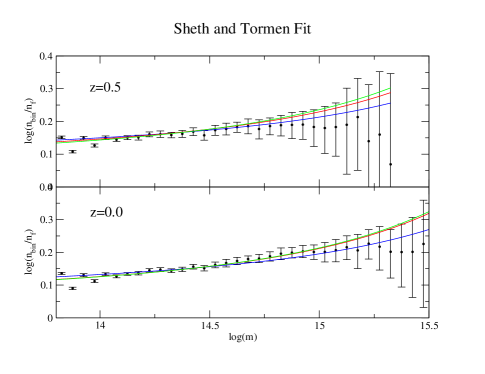
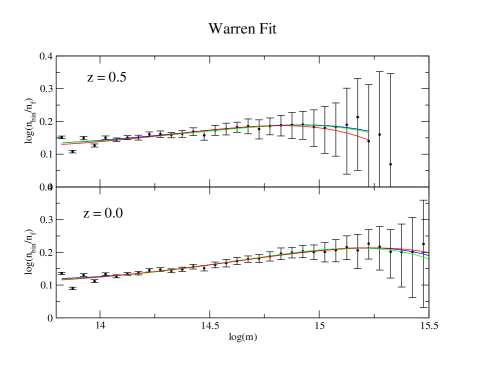
Figure 6: Mass functions when the link length is 0.2, divided by a fiducial curve; three curves show fits to equation 19 and 20 returned by our three algorithms:   $\chi^{2}$-fit (green), Poisson ML fit (red), and new ML fit (blue). Error bars show rms between variation between simulations.

Of our three fitting methods two are standard and one is new. The two standard methods compare the theoretical model with a binned halo mass function, and both assume Poisson counts in a bin. But, whereas one approach computes a simple chi-square of the difference between the expected and measured counts in bins (e.g. Jenkins et al., 2001; Reed et al., 2007), the other uses a Maximum Likelihood approach (Warren et al., 2006). These methods are slightly less than ideal, because there is some art in choosing the size of the bin. In the Appendix, we describe our new method, which is a Maximum Likelihood estimator that does not work with binned counts.

Since the Poisson assumption is an important ingredient in the first two methods (our new method makes an equivalent assumption), it is important to check if this assumption is accurate.   Figure 5 shows the ratio of the variance between runs to the mean count (determined by averaging over all the runs) in each bin.   If the counts are truly Poisson, then this ratio should be unity, with a typical spread of about $\sqrt{2/(N-1)}$, where $N$ is the number of runs from which the mean and variance were estimated (this assumes $N\gg 1$ is large).   The Figure shows that the Poisson assumption is good, although there is a hint that the variance drops below the Poisson value for the most massive halos.

To minimize systematic effects due to the finite mass resolution of the simulation we only fit the mass function for halos with more than 105 particles:  i.e., $M\simeq 6.310^{13}h^{-1}M_{\odot}$. For the two fitting methods that require binned counts, the bin widths were 0.05 dex, except for the highest mass bin, which was enlarged to include at least 80 halos (in most cases this last bin contains more than 200 halos). For each bin, the rms of the 49 simulations was used as a weight when performing the chi-square fit. Figure 6 shows the results; all three estimators return similar fits to the measurements.

In practice, when fitting to equation (19), the best-fit $p$ and $q$ values vary little from one simulation to another, so if one averages $p$ and $q$ over the 49 runs, then the mass function associated with these averaged values is a good description of the average measured mass function.   Table 2 shows the mean and rms dispersion of $p$ and $q$, derived from averaging the best fit values for each of the 49 simulations.

The uncertainties in $p$ and $q$ are correlated.   We argue in the Appendix that this may be understood, at least for our new estimator, in terms of the mass fraction that is predicted to lie above our minimum mass threshold (following Sheth et al., 2003).   This quantity is very well measured in each simulation and, for the case of equation (19), this means that the best fit $p$ and $q$ are expected to lie along a simple well-defined curve, and they do.)

Reporting our results of fitting to equation (20) is less straightforward.  This is because this functional form has four free parameters, so two other measured quantities are required for tracking correlation between parameters. The most natural candidates are the mean and mean square mass of the halos that are above threshold.   These constraints give rise to a complicated set of islands in parameter space, thus compromising any attempt to describe the uncertainty range on the best fit parameters in terms of simple lower and upper limits.  (I.e., if one rises slightly above the level of the global minimum, one includes many other local minima.) In this case, the curves we show are for the parameters obtained by combining the halo catalogs from all the individual simulations, and then performing the fit. Figure 15 illustrates. Notice that the parameter $c$ is rather well constrained, whereas the other two are not. This is because we are essentially only fitting the high mass end, where the counts are falling exponentially and the parameters $a$ and $b$ matter little. Indeed, whereas the various best-fit parameter combinations all produce essentially the same counts at the lowest masses we probe, they differ (slightly) only at high masses.

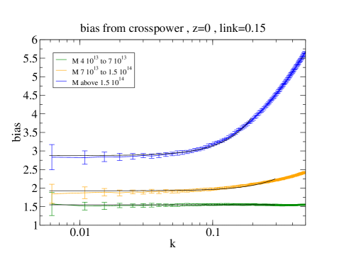
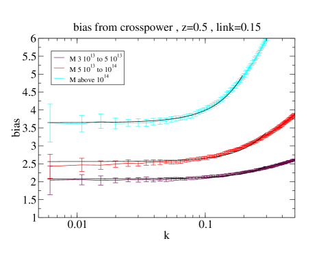
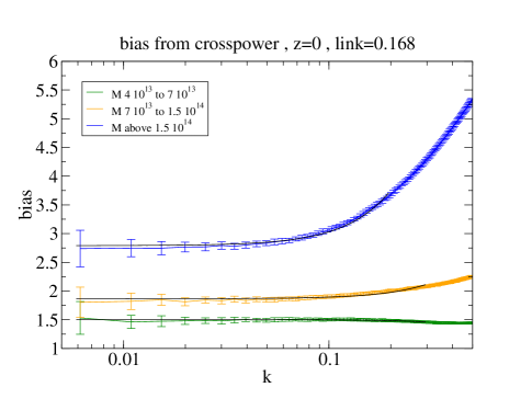
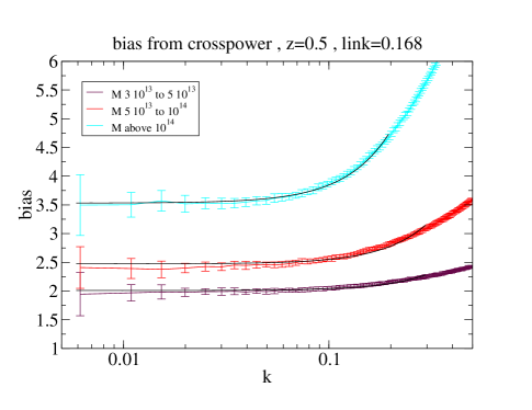
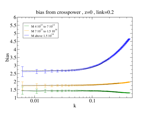
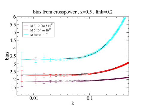
Figure 7: Halo-mass bias from cross power spectra. Left panels show results        at $z=0$; right panels at $z=0.5$.        From top to bottom, linking lengths are 0.15, 0.168 and 0.2. Error bars show rms variation between simulations. Black solid lines are fits to the k dependence of bias between $k=[0.006,0.2]$ for the highest mass bins and $k=[0.006,0.3]$ for the other mass bins.

Before concluding this section, it is worth noting that, for a given link-length, the value of $p$ changes little with $z$. In contrast, for a fixed $z$, the value of $p$ decreases systematically as $l_{\rm link}$ increases, suggesting that the intuitively appealing notion of the set of particles linked together by longer link-lengths at an earlier time being the same as the set linked together by a shorter link-length at a later time, is not correct in detail.

3.4 Halo-mass cross power-spectra

For the reasons discussed earlier, we have measured the halo-mass cross power spectra for all our halo catalogs, and so obtained the large scale bias for different halo mass bins.

Mass range:				Low			Medium			High
$z$	$l_{\rm link}$	$q$	$p$	$b_{1}$	$b_{2}$	$b_{3}$	$b_{1}$	$b_{2}$	$b_{3}$	$b_{1}$	$b_{2}$	$b_{3}$
0.	0.15	0.82	0.289	1.6	-0.2589	-1.422	1.914	0.1515	-3.134	2.728	2.468	-6.795
0.	0.168	0.773	0.272	1.534	-0.3326	-1.111	1.83	0.01092	-2.675	2.616	2.094	-6.378
0.	0.2	0.709	0.248	1.442	-0.4203	-0.7046	1.715	-0.1604	-2.061	2.461	1.619	-5.734
0.5	0.15	0.842	0.288	2.079	0.4327	-4.113	2.481	1.385	-6.54	3.435	5.32	-8.319
0.5	0.168	0.792	0.269	1.982	0.24	-3.556	2.361	1.056	-5.868	3.28	4.598	-8.311
0.5	0.2	0.724	0.241	1.847	0.003493	-2.801	2.196	0.6481	-4.912	3.066	3.679	-8.028

Table 3: Peak-background split bias factors (Appendix B gives    explicit expressions) with the free parameters $p$ and $q$ obtained    from using our new ML method to fit the halo abundances to    equation (19) (see Table 2).

$z$	$l_{\rm link}$	$M_{\rm min}$	$M_{\rm max}$	bias	rms	$b_{\nu}$	$b_{\zeta}$
0.0	0.15	4	7	1.53	0.05	1.55	0.02
0.0	0.15	7	15	1.89	0.05	1.93	3.67
0.0	0.15	15	$10^{5}$	2.88	0.06	2.87	26.4
0.5	0.15	3	5	2.05	0.06	2.08	3.88
0.5	0.15	5	10	2.50	0.06	2.56	9.10
0.5	0.15	10	$10^{5}$	3.64	0.11	3.64	35.5
0.0	0.168	4	7	1.48	0.05	1.50	-0.45
0.0	0.168	7	15	1.83	0.05	1.87	2.81
0.0	0.168	15	$10^{5}$	2.79	0.06	2.79	24.1
0.5	0.168	3	5	1.99	0.06	2.01	3.11
0.5	0.168	5	10	2.42	0.07	2.47	7.73
0.5	0.168	10	$10^{5}$	3.52	0.09	3.53	31.5
0.0	0.2	4	7	1.42	0.06	1.43	-1.13
0.0	0.2	7	15	1.74	0.06	1.77	1.69
0.0	0.2	15	$10^{5}$	2.67	0.06	2.68	20.9
0.5	0.2	3	5	1.88	0.06	1.90	1.86
0.5	0.2	5	10	2.26	0.06	2.30	5.46
0.5	0.2	10	$10^{5}$	3.28	0.08	3.29	25.8

Table 4: Large-scale bias for three bins in halo mass.        Halo masses are in units of $10^{13}h^{-1}M_{\sun}$.      The bias was measured from the halo-mass cross spectrum at      $k=0.03~{}h/{\rm Mpc}$, while the parameters $b_{\nu}$ and $b_{\zeta}$      are a fit to the scale dependence of the bias between      $k=[0.006,0.2]$ for the high mass bin and $k=[0.006,0.3]$      for the other two mass bins.         

Figure 7 shows the ratio of $P_{\rm hm}$ to the power spectrum of the mass at $z=0$ for three bins in halo mass. The three panels show results for the three linking lengths. In all cases, for $k$ below $0.05h^{-1}$Mpc, the bias is approximately independent of $k$. (The strong $k$-dependence at larger $k$ is consistent with previous work, e.g., Sheth & Tormen, 1999).   This large scale bias is largest for the halo catalog from the shortest linking length.  This is not surprising, since the bias is expected to increase with halo mass, and a halo of a given mass with this length will only be more massive when the link length is longer. Thus, for example, halos at the high end of the middle mass bin may have been in the larger mass bin when the link length was longer. Their stronger clustering increases the bias for the small link-length catalogs.

If we had found that the longer link-length halo catalogs from an earlier time were essentially the same as the shorter link-length catalogs at a later time, then we would be able to use the continuity equation to relate the bias of the high-$z$ long-$l_{\rm link}$ objects to the bias of the low-$z$ short-$l_{\rm link}$ objects.   Although not exact, this should still give a good qualitative idea of the bias:  $(b_{z}-1)=(b_{0}-1)(D_{0}/D_{z})$ so, for $b_{1}>1$, we expect the high-$z$ sample to have a larger bias factor.

3.5 Relation to peaks bias

In view of our discussion of peaks bias, we have fitted our measurements to functions of the form $b_{\nu}+b_{\zeta}k^{2}$. These parameters are reported in Table 4 together with the value of the bias at $k=0.03h^{-1}$Mpc and its rms error.  In most cases, the quadratic form is not a good fit to the $k$-dependent bias at $k>0.2h$Mpc^-1 – the $k$-dependence is weaker.  However, Table 4 shows that the amplitude of the quadratic piece increases rapidly as $m$ increases, in qualitative agreement with expectations.

We have found that the radii $R_{pk}$ required to match the values of $b_{\nu}$ and $b_{\zeta}$ in the large scale $\nu$ limit (equation 38 in Desjacques (2008)) are about $8-9h^{-1}$Mpc for the largest mass bin, and smaller for the other bins.   These radii are comparable to the initial Lagrangian radii of the halos, so they are not unreasonable.  However, to see if the scaling with mass is quantitatively correct, we should account more carefully for how the range in halo masses maps to that in peak smoothing scales, as well as for the effects of nonlinear evolution on $b_{\nu}$ and $b_{\zeta}$.  This is beyond the scope of our paper.

3.6 Comparison with predicted large-scale bias

We are now in a position to compare the measured large scale bias factor with that predicted from fitting the mass function and applying the peak background split to estimate $b_{1}$.   The peak-background split prediction is

$$b_{1}\equiv 1-\frac{\partial\ln{\rm d}n/{\rm d}m}{\partial\delta_{c}},$$ (21)

so $b_{1}$ associated with equations (19) and (20) is

$$b_{1}^{ST} = 1+\frac{q\nu-1}{\delta_{c}}+\frac{2p/\delta_{c}}{1+(q\nu)^{p}} \qquad{\rm and}$$ (22)

$$b_{1}^{W} = 1+\frac{c\nu-1}{\delta_{c}}       +\frac{2ab+b+(c\nu)^{a}}{\delta_{c}\,(b+(c\nu)^{a})}.$$ (23)

The thick solid lines in Figure 8 show the measurement, $P_{\rm hm}/P_{\rm mm}$ at $k=0.03~{}h$Mpc^-1. The thickness of the lines shows the two-$\sigma$ range for the measurement, i.e., two times the error on the mean value. Each triple of symbols shows the predicted bias ($b_{1}$ of equation 22) associated with our three ways of fitting the mass function to equation (19).   Clearly, they give similar results. The error bars show the scatter in the predicted peak-background split bias between the 49 simulations (i.e., we use the best fit $p$ and $q$ obtained from fitting the halo abundances in a simultion to predict its $b_{1}$; the scatter in $p$ and $q$ between simulations translates into scatter in $b_{1}$).   The upper and lower panels show results at $z=0$ and $z=0.5$ respectively.

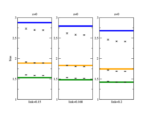
Figure 8: Comparison of measured large scale bias factor (thick solid line)   with the predicted $b_{1}$ of equation (22), for the same three   bins in halo mass shown in the previous figure (higher masses have   larger bias factors).  The parameters $p$ and $q$ of $b_{1}$ are   obtained from fitting the mass function to equation (19).     For each mass bin, the three symbols with error bars show the   predictions associated with our three ways of fitting the mass   function; the error bars show the scatter in the bias between   the 49 simulations, divided by $\sqrt{49}$.   Upper panel shows results at $z=0$, lower panel at $z=0.5$.

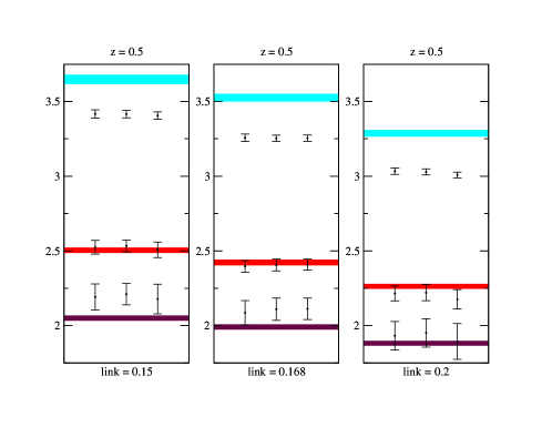
Figure 9: Same as previous figure, but now $b_{1}$ is from         equation (23), with parameters from fitting the mass         function to equation (20).

The differences between the measurements and the predicted values of $b_{1}$ are statistically significant, especially for masses which are large compared to $M_{*}$.  Figure 9 shows that this is not due to the parametric form assumed for the halo mass function: fitting to equation (20) and using the associated expression for $b_{1}$ (equation 23), yields similar results.  (There is one obvious difference:  at high masses, the uncertainty on the predicted $b_{1}$ is similar to that associated with equation 22, but at lower masses, the uncertainty associated with equation 23 is substantially larger.  This is because, at high masses, both formulae for $b_{1}$ are sensitive only to the scale of the exponential cut-off in halo counts, which is determined by the parameters $q$ and $c$ respectively.   At lower masses, the other parameters also matter, of which there are more for equations 20 and 23 than for equations 19 and 22.)   We find qualitatively similar effects for all our choices of $l_{\rm link}$.

What should we make of the discrepancy between the measured large scale bias and $b_{1}$ at high masses?  Following the discussion of Section 2.3, such differences are not unexpected, because the peak-background split bias relation is nonlinear.   As a result, the expected large scale bias factor $b_{\times}$ depends on the higher order bias parameters $b_{2}$ and $b_{3}$ as well as $b_{1}$ (see equation 11).  Like $b_{1}$, these also depend on halo mass, and the parametrization of the halo mass function.   Explicit formulae are provided in Appendix B, and Table 3 provides the numerical values associated with the fits to equation (19).

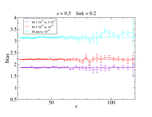
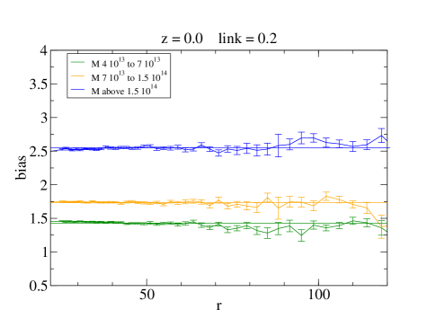
Figure 10: Configuration space estimate of halo bias,          $\sqrt{\xi_{hh}/\xi_{dm}}$, for the same mass bins        as in previous Figures, when $l_{\rm link}=0.2$ at           $z=0.5$ (left) and $z=0$ (right). Error bars show the error on the mean value betweeen simulations.

Unfortunately, the expected difference depends on a smoothing scale $R$ for which we have no underlying theory.  On the other hand, equation (10) shows that we expect $b_{\times}\approx b_{1}$ for our lower mass bins, but that $b_{\times}\geq b_{1}$ at very large masses, in qualitative agreement with our measurements.  (For lower masses than we are studying here, we expect $b_{\times}\leq b_{1}$.) Therefore, we have treated $R$ as a free parameter, to allow equation (11) for $b_{\times}$ to fit as well as possible.  The predicted difference between $b_{\times}$ and $b_{1}$ which results sometimes has the wrong sign, because $b_{3}$ can be large and negative (see Table 3).   The differences at large masses are qualitatively consistent with our measurements if we ignore higher order terms in $\sigma^{4}$ and we set $b_{3}=0$, although there is no theoretical justification for either of these steps.  And if we do this, then we are unable to match the measurements at lower masses.   Thus, while equation (11) can sometimes account qualitatively for the differences seen in Figures 8 and 9 ($b_{2}$ and $b_{3}$ are both negative in the low-mass limit), it cannot account in detail for the observed differences.  This suggests that the deterministic nonlinear local bias model does not provide a sufficiently accurate description of halo bias.

3.7 Comparison with bias from configuration space

So far we have been measuring the large scale bias from simulations in Fourier space using $P_{hm}$.  But one can also measure it in configuration space from the correlation function $\xi_{hh}/\xi_{dm}$. Figure 10 shows $\sqrt{\xi_{hh}/\xi_{dm}}$ for the same three halo mass bins when $l_{\rm link}=0.2$.  Error bars show the error on the mean value between simulations.  A constant bias is a good description of the measurement on scales between $25-75h^{-1}$Mpc. The average value of this ratio, computed between $r=[40,60]h^{-1}$Mpc, is shown by the solid horizontal lines.   At scales close to the acoustic peak (105$h^{-1}$Mpc for our cosmological model) the bias has some scale dependence, particularly for the highest mass halos, which we discuss shortly.

Figure 11 compares the Fourier space measurement of $P_{hm}/P_{mm}$ (bars on the left of each panel), with the mean and dispersion of $\sqrt{\xi_{hh}/\xi_{dm}}$ (thick solid bars on right of each panel).  (Recall that, for each simulation, these ratios are averaged over the range $r=[40,60]h^{-1}$Mpc.)  The widths of the bars show the $2\sigma$ error on the mean measured bias (i.e, the rms dispersion times $2/\sqrt{49}$), indicating that these two measures of the bias are slightly but significantly different for the highest mass bin.  Each pair of error bars shows the two peak background split predictions for $b_{1}$ (equations 22 and 23, and recall that the latter has substantially larger uncertainties) for each of the three methods we use when fitting the mass function (from left to right, these are New ML, Poisson ML, $\chi^{2}$-method).  Notice that the predictions are closer to the configuration space measurement than the other one, but the difference is still significant.

Unfortunately, it is not straightforward to compare $b_{\xi}$ of equation (12) with our measurements, because the theory calculation is for the correlation function of the smoothed halo field (divided by that of the similarly smoothed mass field), whereas our measurements of $\xi_{hh}$ and $\xi_{dm}$ are made on the unsmoothed point distributions.   Nevertheless, because we measure $b_{\xi}<b_{\times}$, and this is qualitatively consistent with equation (12), we might ask what effective smoothing radius is required to explain the difference.   For our large mass bins, this radius is of order $R\sim 40h^{-1}$Mpc.   However, although this would make $b_{\xi}=b_{\times}$, it does not explain the magnitude of the difference from $b_{1}$.

We noted that the halo bias has some scale dependence around the acoustic peak scale (105$h^{-1}$Mpc for our cosmological model).   This scale dependent halo bias is consistent with the trends reported in (Smith et al., 2007, 2008) that have since been confirmed by a number of authors (Sánchez et al., 2008; Sanchez et al., 2009; Kim et al., 2008).

3.8 Halos from spherical overdensity

It is well known that some objects identified by a Friends of Friends algorithm may have dumb-bell like shapes.  In this case, the algorithm labels as a single massive object what might better be classified as two separate objects of smaller mass.  This changes how the abundance and the clustering depend on mass, so one might wonder if some of the discrepancy with the peak-background split predictions we find can be attributed to our choice of group-finder.

In this section, we perform the same analysis as before, but now using halos identified with a spherical overdensity (SO) requirement.   Halos were identified as spherical regions, each 200 times denser than the background, in the $z=0$ outputs of our simulations by J. Tinker following standard methods.   We compute the abundance, cross-power bias $b_{\times}$, and autocorrelation bias $b_{\xi}$ for three bins in halo mass.   Whereas the two higher mass bins are the same as before, the lowest mass bin is slightly different, due to details of how the halo finder was run.   Results for these measured bias factors are shown as bars in Figure 12, together with the peak-background split prediction from their mass function (black dots with error bars). These show that $b_{\times}$ is about 5% larger than $b_{\xi}$, which is itself larger than the peak-baground split prediction.   These are in the same sense, and have the same magnitude as our previous results based on FoF halos (Figure 11).   As an extra test we have computed $b_{1}$ for the higher mass bin by fiting the mass funcion of SO halos only in the mass bin range instead of the wider range available. In this case the difference between $b_{1}$ and $b_{\xi}$ got reduced to half, but it remains still significant. We conclude that our finding that $b_{1}\neq b_{\times}\neq b_{\xi}$ does not depend on how halos were identified.

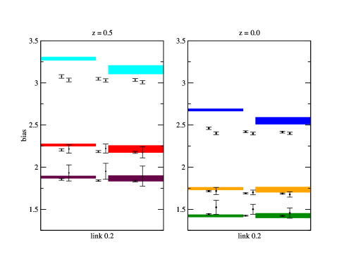
Figure 11: Comparison of large scale bias estimates for the same halo mass   bins as in previous figures when $l_{\rm link}=0.2$.  Thick bars   show the measured $P_{hm}/P_{mm}$ (left) and   $\sqrt{\xi_{hh}/\xi_{mm}}$ (right), and symbols with error bars show   the linear bias parameter $b_{1}$ predicted from the peak background split.

4 Discussion and conclusions

The peak-background split argument is commonly used to relate the abundances of dark matter halos to their spatial clustering. We have found that this estimate of the bias between halos and the dark matter is not accurate to better than $\sim 10$ percent when compared with different measures of large scale bias, particularly for the most massive halos.  We did not test the intermediate or low mass regime.

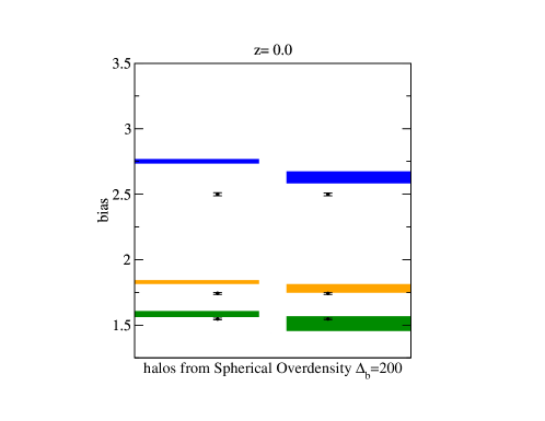
Figure 12: Same as previous figure, but now for halos identified using   an SO algorithm.  Results are shown for the same mass bins as before,   except that the lowest mass bin is from $5.93\cdot 10^{13}M_{\odot}$ to $7.0\cdot 10^{13}M_{\odot}$.     Thick bars show the measured $P_{hm}/P_{mm}$ (left)   and $\sqrt{\xi_{hh}/\xi_{mm}}$ (right); the thickness of the bars   indicates the two-$\sigma$ range.   Symbols with error bars show the linear bias parameter $b_{1}$   predicted from fitting equation (19) to the halo   abundances using the Poisson and $\chi^{2}$ methods.     Error bars show the rms scatter between realizations.

Our results are insensitive to a) how exactly we define halos, b) the exact functional form of the mass function and c) how the mass function was fitted. We have checked this by exploring three friends-of-friends linking lengths for defining the halo catalogs, 0.15, 0.168 and 0.2 (see Figures 1–4), as well as using a spherical overdensity criterion (Section 3.8); two functional forms for the mass function (equations 19 and 20, for which the associated linear bias factors $b_{1}$ are given by equations 22 and 23); and three methods for fitting halo counts to these functional forms, one of which is new.   The latter is a likelihood estimator that maximizes the probability that a randomly chosen particle belongs to a halo of specified mass; it does not require binned halo counts, thus removing the arbitrariness of the choice of bin size which is intrinsic to more standard methods.

We have also studied the self-similarity of the mass function at different linking lengths for $z=0,0.5,1$ and find that it is qualitatively but not exactly self-similar (see Figure 4). We have argued that this difference may be reduced by scaling the linking-length as a function of redshift as suggested by the spherical collapse model.

Results for the different estimates of large-scale halo bias are shown for two different redshifts in Figures 8 and 9.  Although halo bias appears to be close to linear on large scales (Figures 7 and 10), the bias factor $b_{\xi}\equiv\sqrt{\xi_{hh}/\xi_{dm}}$ one measures at large $r$ is different from $b_{\times}\equiv P_{hm}/P_{mm}$ measured at small $k$, and both are different from the peak-background split estimate of the linear bias factor $b_{1}$, at large masses where $b_{1}\geq 2$ (Figures 11 and 12).   On the other hand, at lower masses where $b_{1}\approx 2$, $b_{1}\approx b_{\times}\approx b_{\xi}$ to within a few percent.

We discussed possible explanations for the differences at large masses.   For example, the contribution of nonlinear bias terms, $b_{2}$, $b_{3}$, etc., which are generic to the peak-background split argument (we provide explicit expressions in Appendix B), make $b_{1}\neq b_{\times}\neq b_{\xi}$ (see equations 10 and 12).   However, the amplitude of these corrections depends on a parameter, $\sigma^{2}$, for which there is no underlying theory, other than the expectation that it is smaller than unity, but greater than zero.   While nonlinear terms could explain the difference between $b_{\xi}$ and $b_{\times}$, the differences between these bias factors and $b_{1}$ are consistent with our measurements only if we ignore terms of order $\sigma_{R}^{4}$ and higher, and we set $b_{3}=0$, although there is no theoretical justification for either of these steps.   But then, to be self-consistent, we should use the same algorithm for the lower mass bins, and there, what (barely) worked for the high masses no longer works (because $b_{2}$ and $b_{3}$ are negative).

Although our analysis was restricted to massive halos, it is likely that our conclusions about the (in)accuracy of the peak background split extend to lower masses.  To illustrate, Figure 13 shows how the predicted $b_{\times}$ differs from the linear bias factor $b_{1}$, for a number of choices of the unknown parameter $\sigma_{R}$.   (To make the plot, we have ignored terms of order $\sigma_{R}^{4}$ and higher in equation 10.)   Note that the difference between $b_{\times}$ and $b_{1}$ is not simple:   at high masses where $b_{1}\geq 2$, $b_{\times}>b_{1}$, whereas the opposite is true at intermediate masses, and $b_{\times}\approx b_{1}$ at very low masses.  In recent simulations which resolve smaller halos (e.g., Boylan-Kolchin et al., 2009), the measured large scale bias is indeed smaller than $b_{1}$, in qualitative agreement with Figure 13.  However, comparison with Fig. 10 of Boylan-Kolchin et al. (2009) shows that, at the 10% level, the quantitative agreement is not good.

Figure 13: Dependence of $b_{\times}$ (equation 10, with terms of order $\sigma_{R}^{4}$ and higher set to zero) on the smoothing parameter $\sigma_{R}^{2}$, when the bias factors $b_{1},b_{2}$ and $b_{3}$ are given by equation (B) with $(p,q)=(0.25,0.7)$.   Solid curve shows the linear bias parameter $b_{1}$, which corresponds to the $\sigma^{2}\to 0$ limit of $b_{\times}$.  

We conclude that more work is needed to understand the nature of halo bias at the few percent level.  Our results suggest that we are beginning to see the limitations of the local deterministic bias model – while the inclusion of higher order bias terms can sometimes explain the qualitative difference between $b_{1}$, $b_{\times}$ and $b_{\xi}$, it does not work quantitatively for all masses. As one alternative, we considered a peaks-bias model which is linear but nonlocal and scale dependent in $k$-space.  More work is needed before a fair quantitative comparison of this model with the measurements can be made, but our measurements suggest qualitative agreement.   Another, which we are pursuing, is to study models in which the evolution between initial and evolved fields (e.g., equation 2) is no longer a deterministic function of the overdensity.

Finally, we note that our expression for the bias factor implicitly assumes that the mass function has a universal form. The fact that it is not quite universal will modify the bias factor predicted by the peak-background split (Sheth & Tormen, 1999), although work in progress suggests this is not enough to explain the discrepancies we have found.

Appendix A Fitting the halo mass function

This Appendix defines a Maximum likelihood estimator of the halo mass function that does not require binned halo counts.  The key is to think about the mass function in exactly the same way that theorists do when modeling it.  Namely, the question is not: How many halos are there in a certain mass bin in the simulation box? but, What is the probability that a randomly chosen particle in the simulation box was in a halo of mass $m$?

Let ${\rm d}n(m)\,{\rm d}m$ denote the number density of haloes of mass $m$.  Then the fraction of particles in such haloes is

$$f(m)\,{\rm d}m=\frac{m}{\bar{\rho}}\,\frac{{\rm d}n(m)}{{\rm d}m}.$$ (24)

Let $f(m|{{\mbox{\boldmath$\theta$}}})\,dm$ denote a theoretical model of this quantity, where $\theta$ denotes the vector of parameters which specifies the model.  Then the likelihood to be maximized is

$${\cal L}({{\mbox{\boldmath$\theta$}}})=\prod_{i=1}^{N_{p}}f(m_{i}|{{\mbox{\boldmath$\theta$}}}),$$ (25)

where the product is over all $N_{p}$ particles in the simulation box.   In practice, one only measures halos down to some minimum mass.   This modifies the estimator above to

$${\cal L}({{\mbox{\boldmath$\theta$}}})=  F(m\leq M_{\rm min}|{{\mbox{\boldmath$\theta$}}})^{N_{p}-N_{m\geq M_{\rm min}}}\   \prod_{i=1}^{N_{p}}f(m_{i}|{{\mbox{\boldmath$\theta$}}}),$$ (26)

where

$$F(m\leq M_{\rm min}|{{\mbox{\boldmath$\theta$}}})\equiv 1-\int_{M_{\rm min}}^{\infty}dm\,f(m|{{\mbox{\boldmath$\theta$}}}),$$ (27)

and $N_{m\geq M_{\rm min}}$ is the total number of particles in halos above the minimum mass.  We have explicitly written this as unity minus the integral over massive halos to allow for the possibility that bound halos below some mass scale may not exist (and because some authors choose functional forms which lead to divergences when integrated over all $m$).  This way of writing the probability shows that it is trivial to account for this possibility.

Now, because one has found the halos, one need not draw from the particle list when computing the likelihood, one can use the (considerably smaller!) halo catalog instead.  I.e.,

$${\cal L}({{\mbox{\boldmath$\theta$}}})=  F(m\leq M_{\rm min}|{{\mbox{\boldmath$\theta$}}})^{N_{p}-N_{m\geq M_{\rm min}}}\   \prod_{i=1}^{N_{h}}f(m_{i}|{{\mbox{\boldmath$\theta$}}})^{N_{i}},$$ (28)

where the product is now over the $N_{h}$ halos in the box, $N_{i}$ is the number of particles in halo $i$, and

$$N_{m\geq M_{\rm min}}=\sum_{i=1}^{N_{h}}N_{i}.$$ (29)

The derivatives of $\ln\,{\cal L}({{\mbox{\boldmath$\theta$}}})$ with respect to the parameters $\theta_{i}$ can be done analytically, so this method is fast.  The second derivatives provide analytic estimates of shape of the likelihood surface near the minimum, and hence of the uncertainties on the best-fit parameters.

In practice, the mass functions of current interest are written in terms of the scaled variable $\nu$.   Therefore, we scale all masses $m$ to $\nu$ using equation (16), and then write the likelihood in these scaled variables before maximizing:

$${\cal L}({{\mbox{\boldmath$\theta$}}})=  F(\nu\leq\nu_{\rm min}|{{\mbox{\boldmath$\theta$}}})^{N_{p}-N_{m\geq M_{\rm min}}}\   \prod_{i=1}^{N_{h}}f(\nu_{i}|{{\mbox{\boldmath$\theta$}}})^{N_{i}}.$$ (30)

It is straightforward but tedious to compute the first and second derivatives with respect to the parameters $\theta$.  Doing so gives an idea of the expected accuracy of and covariances between the best-fitting parameters.  However, a more intuitive demonstration of the covariances can be got by noting that, for large $M_{\rm min}$, the vast majority of particles in the simulation are not assigned to halos, and so the line of degeneracy is driven by requiring that the model always produce the observed mass fraction in halos. For example, when fitting to equation (19), the parameters $p$ and $q$ must change so as to keep $A_{p}\,[\Gamma(1/2,q\nu_{\rm min}/2,\infty)/\Gamma(1/2)+2^{-p}\Gamma(1/2-p,q\nu_{\rm min}/2,\infty)/\Gamma(1/2)]$ fixed. The solid line in Figure A1 shows this curve for halos of mass $M>6.31\times 10^{13}h^{-1}M_{\odot}$ identified with $l_{\rm link}=0.2$ at $z=0$, at which time the mass fraction in halos is 0.13 (this is the mean over all 49 simulations; the actual fraction varies slightly from one realization to another).   Symbols show the best fit parameters for each of the 49 simulations.

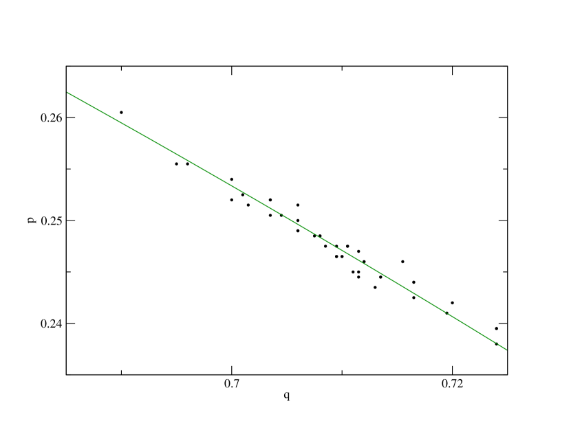
Figure 14: Best fit $p$ and $q$ parameters of equation (19) for each of the 49 simulations with linking-length 0.2 and redshift $z=0$. The solid line shows a constant fraction of mass in halos equal to the mean of all simulations.

Figure 15 shows a similar comparison of the measured covariances between best fit parameters of equation (20). We have not shown the expected correlations for this case.

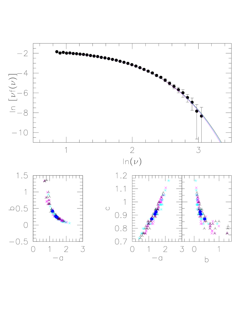
Figure 15: Top: Measured $z=0$ halo abundances (link length 0.2) when the 49 simulations have been combined. Error bars show the rms variation between simulations. Curves show the result of fitting equation (20) to the counts using the three methods described in the main text. All methods return essentially the same counts at the lowest $\nu$ we probe; they differ slightly at higher $\nu$. Bottom: Covariance between best-fit parameters for each of the 49 simulations with linking-length 0.2 and redshift $z=0$. The fractional error on $c$ is much smaller than on the other parameters. Stars, crosses and tripods show results for the ML, Poisson and $\chi^{2}$ methods: there is no systematic trend with fitting method. Filled solid circles show the parameters associated with fitting to the combined counts.

Appendix B Bias factors

In the peak background split ansatz, one writes the halo fluctuation $\delta_{h}$ as a power series of the mass fluctuation:

$$\delta_{h}=\sum_{i}\frac{b_{i}}{i!}\,\delta^{i},$$ (31)

and one obtains the coefficients $b_{i}$ by taking appropriate derivatives of the halo mass function, and accounting for the fact that halo abundances are estimated in the initial field $\delta_{0}$ rather than the evolved field $\delta$ (Mo & White, 1996; Mo et al., 1997; Sheth & Tormen, 1999).    Namely, one assumes there is a deterministic mapping between $\delta_{0}$ and $\delta$:

$$\delta_{0}=\sum_{i>0}a_{i}\delta^{i},$$ (32)

and that this mapping is given by the spherical evolution model

$$a_{1}=1,\ a_{2}=-\frac{17}{21},\ a_{3}=\frac{341}{567},\ {\rm and}\ a_{4}=-\frac{55805}{130977}.$$ (33)

Then,

$$b_{1}(\nu) = 1+\epsilon_{1}+E_{1}$$

$$b_{2}(\nu) = 2(1+a_{2})(\epsilon_{1}+E_{1})+\epsilon_{2}+E_{2}$$

$$b_{3}(\nu) = 6(a_{2}+a_{3})(\epsilon_{1}+E_{1})+3(1+2a_{2})(\epsilon_{2}+E_{2})$$

$$+\epsilon_{3}+E_{3}$$ (34)

$$b_{4}(\nu) = 24(a_{3}+a_{4})(\epsilon_{1}+E_{1})+$$

$$+12(a_{2}^{2}+2(a_{2}+a_{3}))(\epsilon_{2}+E_{2})+$$

$$+4(1+3a_{2})(\epsilon_{3}+E_{3})+\epsilon_{4}+E_{4}$$

where

$$\epsilon_{1} = \frac{q\nu-1}{\delta_{c}},\qquad\epsilon_{2} = \frac{q\nu (q\nu-3)}{\delta_{c}^{2}},$$

$$\epsilon_{3} =  \frac{q\nu \left(q^{2}\nu^{2}-6q\nu+3\right)}{\delta_{c}^{3}},$$

$$\epsilon_{4} = \frac{q^{2}\nu^{2}\left(q^{2}\nu^{2}-10q\nu+15\right)}{ }                   {\delta_{c}^{4}},$$

$$E_{1} = \frac{2p}{\delta_{c}(q\nu)^{p}+\delta_{c}},\qquad\frac{E_{2}}{E_{1}} = \frac{2p+2q\nu-1}{\delta_{c}},$$ (35)

$$\frac{E_{3}}{E_{1}} =  \frac{4p^{2}+6q\nu p+3q^{2}\nu^{2}-6q\nu-1}{ }                         {\delta_{c}^{2}},$$

$$\frac{E_{4}}{E_{1}} = \frac{2\left(4p^{3}+(8q\nu+4)p^{2}                             +\left(6q^{2}\nu^{2}-6q\nu-1\right)p\right)}{ }                         {\delta_{c}^{3}},$$

$$\ +\frac{2(2q^{3}\nu^{3}-9q^{2}\nu^{2}+q\nu-1)}{\delta_{c}^{3}}$$

for the mass function of equation (19) (Scoccimarro et al., 2001).

For the functional form of equation (20),

$$\epsilon_{1} = \frac{c\nu}{\delta_{c}},\qquad\epsilon_{2} = \frac{c\nu (c\nu-1)}{\delta_{c}^{2}},\qquad\epsilon_{3} = \frac{c^{2}\nu^{2}(c\nu-3)}{\delta_{c}^{3}},$$

$$\epsilon_{4} = \frac{c^{2}\nu^{2}\left(c^{2}\nu^{2}-6c\nu+3\right)}{ }                   {\delta_{c}^{4}},$$

$$E_{1} = \frac{2ab}{\delta_{c}(c\nu)^{a}+b\delta_{c}},\qquad\frac{E_{2}}{E_{1}} = \frac{2a+2c\nu+1}{\delta_{c}},$$ (36)

$$\frac{E_{3}}{E_{1}} = \frac{4a^{2}+6c\nu a+6a+3c^{2}\nu^{2}+2}{\delta_{c}^{2}},$$

$$\frac{E_{4}}{E_{1}} = \frac{2\left(4a^{3}+4(2c\nu+3)a^{2}+                     \left(6c^{2}\nu^{2}+6c\nu+11\right)a\right)}{ }                   {\delta_{c}^{3}},$$

$$+\frac{2(2c^{3}\nu^{3}-3c^{2}\nu^{2}+c\nu+3)}{\delta_{c}^{3}}.$$

We note that the assumption of equation (32) is strong, and only an approximation in triaxial collapse models (Ohta et al., 2004; Lam & Sheth, 2009).  Accounting for this is the subject of ongoing work.

References

- Bardeen et al. (1986) Bardeen J., Bond J., Kaiser N., Szalay A., 1986, Astrophys. J., 304, 15
- Bernardeau (1996) Bernardeau F., 1996, ”Astron. Astrophys.”, 312, 11
- Bond et al. (1991) Bond J. R., Cole S., Efstathiou G., Kaiser N., 1991, Astrophys. J., 379, 440
- Boylan-Kolchin et al. (2009) Boylan-Kolchin M., Springel V., White S. D. M., Jenkins A., Lemson G., 2009, ArXiv e-prints 0903.3041
- Cole & Kaiser (1989) Cole S., Kaiser N., 1989, Mon. Not. Roy. Astr. Soc., 237, 1127
- Cooray & Sheth (2002) Cooray A., Sheth R. K., 2002, Phys. Rept., 372, 1
- Crocce et al. (2006) Crocce M., Pueblas S., Scoccimarro R., 2006, Mon. Not. Roy. Astron. Soc., 373, 369
- Desjacques (2008) Desjacques V., 2008, Phys. Rev., D78, 103503
- Desjacques & Sheth (2009) Desjacques V., Sheth R. K., 2009, Phys. Rev. D
- Fry & Gaztanaga (1993) Fry J. N., Gaztanaga E., 1993, ApJ, 413, 447
- Gaztanaga et al. (2002) Gaztanaga E., Fosalba P., Croft R. A. C., 2002, ”Mon. Not. Roy. Astron. Soc.”, 331, 13
- Jenkins et al. (2001) Jenkins A., Frenk C. S., White S. D. M., Colberg J. M., Cole S., Evrard A. E., Couchma n. H. M. P., Yoshida N., 2001, Mon. Not. Roy. Astron. Soc., 321, 372
- Kaiser (1984) Kaiser N., 1984, Astrophys. J., 284, L9
- Kim et al. (2008) Kim J., Park C., Gott J. R. I., Dubinski J., 2008, ArXiv e-prints
- Lam & Sheth (2009) Lam T. Y., Sheth R. K., 2009, Mon. Not. Roy. Soc. Astr., 395, 1743
- Lee & Shandarin (1998) Lee J., Shandarin S. F., 1998, ApJ, 500, 14
- Manera & Gaztañaga (2009) Manera M., Gaztañaga E., 2009, paper in preparation.
- Martino & Sheth (2009) Martino M. C., Sheth R. K., 2009, Mon. Not. Roy. Astron. Soc., 394, 2109
- Matsubara (1999) Matsubara T., 1999, Astrophy. J, 525, 543
- Mo et al. (1997) Mo H. J., Jing Y. P., White S. D. M., 1997, Mon. Not. Roy. Astron. Soc., 284, 189
- Mo & White (1996) Mo H. J., White S. D. M., 1996, Mon. Not. Roy. Astron. Soc., 282, 347
- Ohta et al. (2004) Ohta Y., Kayo I., Taruya A., 2004, ApJ, 608, 647
- Peacock & Smith (2000) Peacock J. A., Smith R. E., 2000, Mon. Not. Roy. Astron. Soc., 318, 1144
- Press & Schechter (1974) Press W., Schechter P., 1974, Astrophys. J., 203, 297
- Reed et al. (2007) Reed D., Bower R., Frenk C., Jenkins A., Theuns T., 2007, Mon. Not. Roy. Astron. Soc., 374, 2
- Reed et al. (2003) Reed D., et al., 2003, Mon. Not. Roy. Astron. Soc., 346, 565
- Sánchez et al. (2008) Sánchez A. G., Baugh C. M., Angulo R., 2008, Mon. Not. Roy. Soc. Astr., 390, 1470
- Sanchez et al. (2009) Sanchez A. G., Crocce M., Cabre A., Baugh C. M., Gaztanaga E., 2009, ArXiv e-prints
- Scoccimarro (1998) Scoccimarro R., 1998, Mon. Not. Roy. Astron. Soc., 299, 1097
- Scoccimarro et al. (2001) Scoccimarro R., Sheth R. K., Hui L., Jain B., 2001, Astrophys. J., 546, 20
- Seljak (2000) Seljak U., 2000, Mon. Not. Roy. Astron. Soc., 318, 203
- Seljak & Zaldarriaga (1996) Seljak U., Zaldarriaga M., 1996, Astrophys. J., 469, 347
- Sheth (2001) Sheth R. K., 2001, Annals of the New York Academy of Sciences, 927, 1
- Sheth et al. (2003) Sheth R. K., Bernardi M., Schechter P. L., Burles S., Eisenstein D. J., Finkbeiner D. P., Frieman J., Lupton R. H., Schlegel D. J., Subbarao M., Shimasaku K., Bahcall N. A., Brinkmann J., Ivezić Ž., 2003, ApJ, 594, 225
- Sheth & Lemson (1999) Sheth R. K., Lemson G., 1999, Mon. Not. Roy. Astron. Soc., 304, 767
- Sheth et al. (2001) Sheth R. K., Mo H. J., Tormen G., 2001, Mon. Not. Roy. Astron. Soc., 323, 1
- Sheth & Tormen (1999) Sheth R. K., Tormen G., 1999, Mon. Not. Roy. Astron. Soc., 308, 119
- Smith et al. (2007) Smith R. E., Scoccimarro R., Sheth R. K., 2007, Phys. Rev., D75, 063512
- Smith et al. (2008) Smith R. E., Scoccimarro R., Sheth R. K., 2008, Phys. Rev. D, 77, 043525
- Smith et al. (2008) Smith R. E., Sheth R. K., Scoccimarro R., 2008, Phys. Rev., D78, 023523
- Springel (2005) Springel V., 2005, Mon. Not. Roy. Astron. Soc., 364, 1105
- Tinker et al. (2008) Tinker J., Kravtsov A. V., Klypin A., Abazajian K., Warren M., Yepes G., Gottlöber S., Holz D. E., 2008, ApJ, 688, 709
- Warren et al. (2006) Warren M. S., Abazajian K., Holz D. E., Teodoro L., 2006, Astrophys. J., 646, 881
- White (2002) White M., 2002, ApJS, 143, 241