Generalised Pinsker Inequalities

Abstract

We generalise the classical Pinsker inequality which relates variational divergence to Kullback-Liebler divergence in two ways: we consider arbitrary $f$-divergences in place of KL divergence, and we assume knowledge of a sequence of values of generalised variational divergences. We then develop a best possible inequality for this doubly generalised situation. Specialising our result to the classical case provides a new and tight explicit bound relating KL to variational divergence (solving a problem posed by Vajda some 40 years ago). The solution relies on exploiting a connection between divergences and the Bayes risk of a learning problem via an integral representation.

1 Introduction

Divergences such as the Kullback-Liebler and variational divergence arise pervasively. They are a means of defining a notion of distance between two probability distributions. The question often arises: given knowledge of one, what can be said of the other? For all distributions $P$ and $Q$ on an arbitrary set, the classical Pinsker inequality relates the Kullback-Liebler divergence $KL(P,Q)$ and variational divergence $V(P,Q)$ by $\mathrm{KL(P,Q)}\geq\frac{1}{2}[V(P,Q)]^{2}$. This simple classical bound is known not to be tight. Over the past several decades a number of refinements have been given (see Appendix A for a summary of past work).

Vajda Vajda1970 posed the question of determining a tight lower bound on KL-divergence in terms of variational divergence. This “best possible Pinsker inequality” takes the form

$$L(V):=\inf_{V(P,Q)=V}\mathrm{KL}(P,Q),\ \ \ \ V\in[0,2).$$ (1)

Recently Fedotov et al. FedotovTopsoe2003 presented an implicit parametric solution of the form of the graph of the bound as $(V(t),L(t))_{t\in\mathbb{R}^{+}}$ where

$$V(t) = t\left(1-\left(\coth(t)-\textstyle\frac{1}{t}\right)^{2}\right),$$ (2)

$$L(t) = \log\left(\frac{t}{\sinh(t)}\right)+t\coth(t)-\frac{t^{2}}{\sinh^{2}(t)}.$$

One can generalise the notion of a Pinsker inequality in at least two ways: 1) replace KL divergence by a general $f$-divergence; and 2) bound the $f$-divergence in terms of the known values of a sequence of generalised variational divergences (defined later in this paper) $(V_{\pi_{i}})_{i=1}^{n}$, $\pi_{i}\in(0,1)$. In this paper we study this doubly generalised problem and provide a complete solution in terms of explicit, best possible bounds.

The main result is given below as Theorem 6. Applying it to specific $f$-divergences gives the following corollary.

Corollary 1

Let $V=V(P,Q)$ denote the variational divergence between the distributions $P$ and $Q$ and similarly for the other divergences in Table 1 below. Then the following bounds for the divergences hold and are tight:

$$h^{2}\geq 2-\sqrt{4-V^{2}};\ \ \mathrm{J}\geq\textstyle 2V\ln\left(\frac{2+V}{2-V}\right);\ \ \Psi\geq\frac{8V^{2}}{4-V^{2}}$$

$$\mathrm{I} \geq \left(\frac{1}{2}\!-\!\frac{V}{4}\right)\ln(2\!-\!V)\!+\!\left(\frac{1}{2}\!+\!\frac{V}{4}\right)\ln(2\!+\!V)\!-\!\ln(2)$$

$$\mathrm{T} \!\!\!\!\!\geq\!\!\!\! \textstyle\ln\left(\frac{4}{\sqrt{4-V^{2}}}\right)-\ln(2)$$

$$\chi^{2} \!\!\!\!\!\geq\!\!\!\! \textstyle\llbracket V<1\rrbracket V^{2}+\llbracket V\geq 1\rrbracket\frac{V}{(2-V)}$$ (3)

$$\mathrm{KL} \!\!\!\!\geq \!\!\min_{\beta\in[V-2,2-V]}\textstyle\left(\frac{V+2-\beta}{4}\right)\ln\left(\frac{\beta-2-V}{\beta-2+V}\right)+$$ (4)

$$\left(\textstyle\frac{\beta+2-V}{4}\right)\ln\left(\textstyle\frac{\beta+2-V}{\beta+2+V}\right).$$

The proof of the main result depends in an essential way on a learning theory perspective. We make use of an integral representation of $f$-divergences in terms of DeGroot’s statistical information—the difference between a prior and posterior Bayes riskDeGroot1962 . By using the relationships between the generalised variational divergence and the 0-1 misclassification loss we are able to use an elementary but somewhat intricate geometrical argument to obtain the result.

The rest of the paper is organised as follows. Section 2 collects background results upon which we rely. The main result of the paper is stated in Section 3 and its proof presented in in Section 4. Appendix A summarises previous work.

2 Background Results and Notation

In this section we collect notation and background concepts and results we need for the main result.

2.1 Notational Conventions

The substantive objects are defined within the body of the paper. Here we collect elementary notation and the conventions we adopt throughout. We write $x\wedge y:=\min(x,y)$, $x\vee y:=\max(x,y)$ and $\llbracket p\rrbracket=1$ if $p$ is true and $\llbracket p\rrbracket=0$ otherwise. The generalised function $\delta(\cdot)$ is defined by $\int_{a}^{b}\delta(x)f(x)dx=f(0)$ when $f$ is continuous at $0$ and $a<0<b$. For convenience, we will define $\delta_{c}(x):=\delta(x-c)$. The real numbers are denoted $\mathbb{R}$, the non-negative reals $\mathbb{R}^{+}$; Sets are in calligraphic font: $\mathcal{X}$. Vectors are written in bold font: $\mathbf{a},\bm{\alpha},\bm{x}\in\mathbb{R}^{m}$. We will often have cause to take expectations ($\mathbb{E}$) over random variables. We write such quantities in blackboard bold: $\mathbb{I}$, $\mathbb{L}$, etc. The lower bound on quantities with an intrinsic lower bound (e.g. the Bayes optimal loss) are written with an underbar: $\underline{L}$, $\underline{\mathbb{L}}$. Quantities related by double integration recur in this paper and we notate the starting point in lower case, the first integral with upper case, and the second integral in upper case with an overbar: $\gamma$, $\Gamma$, $\bar{\Gamma}$.

2.2 Csiszár $f$-divergences

The class of $f$-divergences (AliSilvey1966, ; Csiszar1967, ) provide a rich set of relations that can be used to measure the separation of the distributions. An $f$-divergence is a function that measures the “distance” between a pair of distributions $P$ and $Q$ defined over a space $\mathcal{X}$ of observations. Traditionally, the $f$-divergence of $P$ from $Q$ is defined for any convex $f:(0,\infty)\to\mathbb{R}$ such that $f(1)=0$. In this case, the $f$-divergence is

$$\mathbb{I}_{f}(P,Q)=\mathbb{E}_{Q}\left[f\left(\frac{dP}{dQ}\right)\right]=\int_{\mathcal{X}}f\left(\frac{dP}{dQ}\right)\,dQ$$ (5)

when $P$ is absolutely continuous with respect to $Q$ and equal $\infty$ otherwise.

All $f$-divergences are non-negative and zero when $P=Q$, that is, $\mathbb{I}_{f}(P,Q)\geq 0$ and $\mathbb{I}_{f}(P,P)=0$ for all distributions $P,Q$. In general, however, they are not metrics, since they are not necessarily symmetric (i.e., for all distributions $P$ and $Q$, $\mathbb{I}_{f}(P,Q)=\mathbb{I}_{f}(Q,P)$) and do not necessarily satisfy the triangle inequality.

Several well-known divergences correspond to specific choices of the function $f$ (AliSilvey1966, , §5). One divergence central to this paper is the variational divergence $V(P,Q)$ which is obtained by setting $f(t)=|t-1|$ in Equation 5. It is the only $f$-divergence that is a true metric on the space of distributions over $\mathcal{X}$ (Khosravifard:2007, ) and gets its name from its equivalent definition in the variational form

$$V(P,Q)=2\|P-Q\|_{\infty}:=2\sup_{A\subseteq\mathcal{X}}|P(A)-Q(A)|.$$ (6)

(Some authors define $V$ without the 2 above.) Furthermore, the variational divergence is one of a family of “primitive” or “simple” $f$-divergences discussed in Section 2.3. These are primitive in the sense that all other $f$-divergences can be expressed as a weighted sum of members from this family.

Another well known $f$-divergence is the Kullback-Leibler (KL) divergence $\mathrm{KL}(P,Q)$, obtained by setting $f(t)=t\ln(t)$ in Equation 5. Others are given in Table 1.

As already mentioned in the introduction, the KL and variational divergences satisfy the classical Pinsker’s inequality which states that for all distributions $P$ and $Q$ over some common space $\mathcal{X}$

$$\mathrm{KL}(P,Q)\geq{\textstyle\frac{1}{2}}[V(P,Q)]^{2}.$$ (7)

2.3 Integral Representations of $f$-divergences

The main tool in our proof of Theorem 6 is the integral representation of $f$-divergences, first articulated by Österreicher and Vajda OsterreicherVajda1993a and Gutenbrunner Gutenbrunner:1990 . They show that an $f$-divergence can be represented as a weighted integral of the “simple” divergence measures

$$V_{\pi}(P,Q)=\mathbb{I}_{f_{\pi}}(P,Q),$$ (8)

where $f_{\pi}(t):=\min\{\pi,1-\pi\}-\min\{1-\pi,\pi t\}$ for $\pi\in[0,1]$.

Theorem 2

For any convex $f$ such that $f(1)=0$, the $f$-divergence $\mathbb{I}_{f}$ can be expressed, for all distributions $P$ and $Q$, as

$$\mathbb{I}_{f}(P,Q)=\int_{0}^{1}V_{\pi}(P,Q)\,\gamma_{f}(\pi)\,d\pi$$ (9)

where the (generalised) function

$$\gamma_{f}(\pi):=\frac{1}{\pi^{3}}f^{\prime\prime}\left(\frac{1-\pi}{\pi}\right).$$ (10)

Recently, this theorem has been shown to be a direct consequence of a generalised Taylor’s expansion for convex functions LieVaj06 ; ReidWilliamson2009 .

Even when $f$ is not twice differentiable, the convexity of $f$ implies its continuity and so its right-hand derivative $f^{\prime}_{+}$ exists. In this case, $\gamma$ is interpreted distributionally in terms of $df^{\prime}_{+}$. For example, when $f(t)=|t-1|$ then $f^{\prime\prime}(t)=2\delta(t-1)$ and so $\gamma_{f}(\pi)=2\frac{1}{\pi^{3}}\delta(1-2\pi)=16\delta_{\frac{1}{2}}(\pi)$.

The divergences $V_{\pi}$ for $\pi\in[0,1]$ can be seen as a family of generalised variational divergences since, $df^{\prime}_{+}(t)$ for any member of this family is $\pi\delta(t-\frac{1-\pi}{\pi})$ and so $\gamma_{f_{\pi}}=\frac{1}{\pi^{2}}\delta_{\frac{1-\pi}{\pi}}$. Thus, for $\pi={\textstyle\frac{1}{2}}$ we have $\gamma_{f_{\frac{1}{2}}}=4\delta_{\frac{1}{2}}$, that is, four times the $\gamma$ function for variational divergence and so by (9) we see that

$$V(P,Q)=4V_{\frac{1}{2}}(P,Q).$$ (11)

Theorem 2 shows that knowledge of the values of $V_{\pi}(P,Q)$ for all $\pi\in[0,1]$ is sufficient to compute the value of $\mathbb{I}_{f}(P,Q)$ for any $f$-divergence, since the weight function $\gamma$ is dependent only on $f$, not $P$ and $Q$. All of the generalised Pinsker bounds we derive are found by asking how knowledge of a the value of a finite number of $V_{\pi}(P,Q)$ constrains the overall value of $\mathbb{I}_{f}(P,Q)$.

Table 1 summarises the weight functions $\gamma$ for a number of $f$-divergences that appear in the literature. These are used in the proof of specific bounds in Corollary 1.

Symbol	Divergence Name	$f(t)$	$\gamma(\pi)$
$\rule{0.0pt}{10.33327pt}V(P,Q)$	Variational	$|t-1|$	$16\delta\left(\pi-\frac{1}{2}\right)$
$\mathrm{KL}(P,Q)$	Kullback-Liebler	$t\ln t$	$\frac{1}{\pi^{2}(1-\pi)}$
$\rule{0.0pt}{10.33327pt}\Delta(P,Q)$	Triangular Discrimination	$(t-1)^{2}/(t+1)$	8
$\rule{0.0pt}{10.33327pt}\mathrm{I}(P,Q)$	Jensen-Shannon	$\frac{t}{2}\ln t-\frac{(t+1)}{2}\ln(t+1)+\ln 2$	$\frac{1}{2\pi(1-\pi)}$
$\rule{0.0pt}{12.91663pt}\mathrm{T}(P,Q)$	Arithmetic-Geometric Mean	$\left(\frac{t+1}{2}\right)\ln\left(\frac{t+1}{2\sqrt{t}}\right)$	$\frac{(2\pi-\frac{1}{2})^{2}+\frac{1}{2}}{4\pi^{2}(\pi-1)^{2}}$
$\rule{0.0pt}{10.33327pt}\mathrm{J}(P,Q)$	Jeffreys	$(t-1)\ln(t)$	$\frac{1}{\pi^{2}(1-\pi)^{2}}$
$\rule{0.0pt}{10.33327pt}h^{2}(P,Q)$	Hellinger	$(\sqrt{t}-1)^{2}$	$\frac{1}{2[\pi(1-\pi)]^{3/2}}$
$\rule{0.0pt}{12.91663pt}\chi^{2}(P,Q)$	Pearson $\chi$-squared	$(t-1)^{2}$	$\frac{2}{\pi^{3}}$
$\rule{0.0pt}{12.91663pt}\Psi(P,Q)$	Symmetric $\chi$-squared	$\frac{(t-1)^{2}(t+1)}{t}$	$\frac{2}{\pi^{3}}+\frac{2}{(1-\pi)^{3}}$

Table 1: Divergences and their corresponding functions $f$ and weights $\gamma$; confer Taneja2005 ; LieVaj06 . Topsøe Topsoe:2000 calls $C(P,Q)=2\mathrm{I}(P,Q)$ and $\tilde{C}(P,Q)=2\mathrm{T}(P,Q)$ the Capacitory and Dual Capacitory discrimination respectively. Several of the above divergences are “symmetrised” versions of others. For example, $T(P,Q)=\frac{1}{2}[\mathrm{KL}(\frac{P+Q}{2},P)+\mathrm{KL}(\frac{P+Q}{2},Q)]$, $I(P,Q)=\frac{1}{2}[\mathrm{KL}(P,\frac{P+Q}{2})+\mathrm{KL}(Q,\frac{P+Q}{2})]$, $\mathrm{J}(P,Q)=\mathrm{KL}(P,Q)+\mathrm{KL}(Q,P)$, and $\Psi(P,Q)=\chi^{2}(P,Q)+\chi^{2}(Q,P)$.

Before we can prove the main result, we need to establish some properties of the general variational divergences. In particular, we will make use of their relationship to Bayes risks for 0-1 loss.

2.4 Divergence and Risk

Let $\underline{\mathbb{L}}(\pi,P,Q)$ denote the 0-1 Bayes risk for a classification problem in which observations are drawn from $\mathcal{X}$ using the mixture distribution $M=\pi P+(1-\pi)Q$, and each observation $x\in\mathcal{X}$ is assigned a positive label with probability $\eta(x):=\pi\frac{dP}{dM}(x)$. If $r=r(x)\in\{0,1\}$ is a label prediction for a particular $x\in\mathcal{X}$, the 0-1 expected loss for that observation is

$$L(r,\pi,p,q)=(1-\pi)q\llbracket r=1\rrbracket+\pi p\llbracket r=0\rrbracket.$$

where $q=\frac{dQ}{dM}(x)$ and $p=\frac{dP}{dM}(x)$ are densities. Thus, the full expected 0-1 loss of a predictor $r:\mathcal{X}\to\{0,1\}$ is given by $\mathbb{L}(r,\pi,P,Q):=\mathbb{E}_{M}[L(r(x),\pi,p(x),q(x))]$ and it is well known (e.g., DevGyoLug96 ) that its Bayes risk is obtained by the Bayes optimal predictor $r^{*}(x):=\llbracket\eta(x)\geq\frac{1}{2}\rrbracket$. That is,

$$\underline{\mathbb{L}}(\pi,P,Q):=\inf_{r}\mathbb{L}(r,\pi,P,Q)=\mathbb{L}(r^{*},\pi,P,Q),$$ (12)

where the infimum is taken over all ($M$-measurable) predictors $r:\mathcal{X}\to\{0,1\}$. So, by the definition of $\eta(x)$ and noting that $\eta\geq\frac{1}{2}$ iff $\pi p\geq\frac{1}{2}(\pi p+(1-\pi)q)$ which holds iff $\pi p\geq(1-\pi)q$ we see that the 0-1 Bayes risk can be expressed as

$$\underline{\mathbb{L}}(\pi,P,Q)$$

$$= \mathbb{E}_{M}[(1-\pi)q\llbracket\eta\geq{\textstyle\frac{1}{2}}\rrbracket+\ \pi p\llbracket\eta<{\textstyle\frac{1}{2}}\rrbracket]$$

$$= (1-\pi)\mathbb{E}_{Q}[\llbracket\pi p\geq(1-\pi)q\rrbracket]+\pi\mathbb{E}_{P}[\llbracket\pi p<(1-\pi)q\rrbracket].$$

We now observe that

$$qf_{\pi}\left(\frac{p}{q}\right)=((1-\pi)\wedge\pi)q-\begin{cases}(1-\pi)q,&q(1-\pi)\leq\pi p\\ \pi p,&q(1-\pi)>\pi p\end{cases}$$

and so by noting that $\mathbb{E}_{Q}\left[f_{\pi}\left(\frac{dP}{dQ}\right)\right]=\mathbb{E}_{M}\left[qf_{\pi}\left(\frac{p}{q}\right)\right]$ we have established the following lemma.

Lemma 3

For all $\pi\in[0,1]$ and all distributions $P$ and $Q$, the generalised variational divergence satisfies

$$V_{\pi}(P,Q) = (1-\pi)\wedge\pi-\underline{\mathbb{L}}(\pi,P,Q).$$ (14)

Thus, the value of $V_{\pi}(P,Q)$ can be understood via the 0-1 Bayes risk for a classification problem with label-conditional distributions $P$ and $Q$ and prior probability $\pi$ for the positive class. This relationship between $f$-divergence and Bayes risk is not new. It was established in a more general setting by Österreicher and Vajda OsterreicherVajda1993a (who note that the term in (14) is the statistical information for 0-1 loss) and later by Nguyen et al. Nguyen:2005 .

2.5 Concavity of 0-1 Bayes Risk Curves

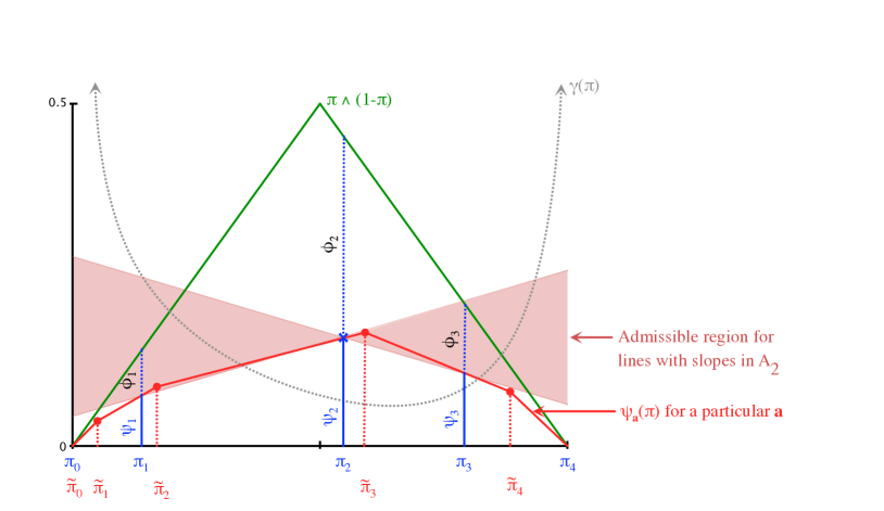
Figure 2: Illustration of construction of optimal $\psi(\pi)=\underline{\mathbb{L}}(\pi,P,Q)$ in the proof of Theorem 6. The optimal $\psi$ is piece-wise linear such that $\psi(\pi_{i})=\psi_{i}$, $i=0,\ldots,n+1$.

For a given pair of distributions $P$ and $Q$ the set of values for $\underline{\mathbb{L}}(\pi,P,Q)$ as $\pi$ varies over $[0,1]$ can be visualised as a curve as in Figure 2.

Lemma 4

For all distributions $P$ and $Q$, the function $\pi\mapsto\underline{\mathbb{L}}(\pi,P,Q)$ is concave.

Proof  By (12) we have that

$$\underline{\mathbb{L}}(\pi,P,Q)=\mathbb{E}_{M}[L(r^{*},\pi,p,q)].$$

Observe that

$$L(r^{*},\pi,p,q) = (1-\pi)q\llbracket\eta\geq{\textstyle\frac{1}{2}}\rrbracket+\pi p\llbracket\eta<{\textstyle\frac{1}{2}}\rrbracket$$

$$= \begin{cases}(1-\pi)q,&q(1-\pi)\leq\pi p\\ \pi p,&q(1-\pi)>\pi p\end{cases}$$

$$= \min\{(1-\pi)q,\pi p\}$$

and so for any $p,q$ is the minimum of two linear functions and thus concave in $\pi$. The full Bayes risk is the expectation of these functions and thus simply a linear combination of concave functions and thus concave.  

The tightness of the bounds in the main result of the next section depend on the following corollary of a result due to Torgersen torgersen1991cse . It asserts that any appropriate concave function can be viewed as the 0-1 risk curve for some pair of distributions $P$ and $Q$. A proof can be found in (ReidWilliamson2009, , §6.3).

Corollary 5

Suppose $\mathcal{X}$ has a connected component. Let $\psi\colon[0,1]\rightarrow[0,1]$ be an arbitrary concave function such that for all $\pi\in[0,1]$, $0\leq\psi(\pi)\leq\pi\wedge(1-\pi)$. Then there exists $P$ and $Q$ such that $\underline{\mathbb{L}}(\pi,P,Q)=\psi(\pi)$ for all $\pi\in[0,1]$.

3 Main Result

We will now show how viewing $f$-divergences in terms of their weighted integral representation simplifies the problem of understanding the relationship between different divergences and leads, amongst other things, to an explicit formula for (1).

Fix a positive integer $n$. Consider a sequence $0<\pi_{1}<\pi_{2}<\cdots<\pi_{n}<1$. Suppose we “sampled” the value of $V_{\pi}(P,Q)$ at these discrete values of $\pi$. Since $\pi\mapsto V_{\pi}(P,Q)$ is concave, the piece-wise linear concave function passing through points

$$\{(\pi_{i},V_{\pi_{i}}(P,Q))\}_{i=1}^{n}$$

is guaranteed to be an upper bound on the variational curve $(\pi,V_{\pi}(P,Q))_{\pi\in(0,1)}$. This therefore gives a lower bound on the $f$-divergence given by a weight function $\gamma$. This observation forms the basis of the theorem stated below.

Theorem 6

For a positive integer $n$ consider a sequence $0<\pi_{1}<\pi_{2}<\cdots<\pi_{n}<1$. Let $\pi_{0}:=0$ and $\pi_{n+1}:=1$ and for $i=0,\ldots,n+1$ let

$$\psi_{i}:=(1-\pi_{i})\wedge\pi_{i}-V_{\pi_{i}}(P,Q)$$

(observe that consequently $\psi_{0}=\psi_{n+1}=0$). Let

$$A_{n} := \left\{\mathbf{a}=(a_{1},\ldots,a_{n})\in\mathbb{R}^{n}\colon\phantom{\frac{\psi_{i+1}-\psi_{i}}{\pi_{i+1}-\pi_{i}}}\right.$$

$$\left.\frac{\psi_{i+1}-\psi_{i}}{\pi_{i+1}-\pi_{i}}\leq a_{i}\leq\frac{\psi_{i}-\psi_{i-1}}{\pi_{i}-\pi_{i-1}},\ i=1,\ldots,n\right\}.$$

The set $A_{n}$ defines the allowable slopes of a piecewise linear function majorizing $\pi\mapsto V_{\pi}(P,Q)$ at each of $\pi_{1},\ldots,\pi_{n}$. For $\mathbf{a}=(a_{1},\ldots,a_{n})\in A_{n}$, let

$$\tilde{\pi}_{i} := \frac{\psi_{i}\!-\!\psi_{i+1}\!+\!a_{i+1}\pi_{i+1}\!-\!a_{i}\pi_{i}}{a_{i+1}-a_{i}},\ i=0,\ldots,n,$$ (16)

$$j := \{k\in\{1,\ldots,n\}:\tilde{\pi}_{k}<\textstyle\frac{1}{2}\leq\tilde{\pi}_{k+1}\}.$$ (17)

$$\bar{\pi}_{i} := \llbracket i<j\rrbracket\tilde{\pi}_{i}+\llbracket i=j\rrbracket\textstyle\frac{1}{2}+\llbracket j<i\rrbracket\tilde{\pi}_{i-1},$$ (18)

$$\alpha_{\mathbf{a},i} := \llbracket i\leq j\rrbracket(1-a_{i})+\llbracket i>{j}\rrbracket(-1-a_{i-1}),$$ (19)

$$\beta_{\mathbf{a},i} := \llbracket i\!\leq\!{j}\rrbracket(\psi_{i}\!-\!a_{i}\pi_{i})\!+\!\llbracket i\!>\!{j}\rrbracket(\psi_{i-1}\!\!-\!a_{i-1}\pi_{i-1})$$ (20)

for $i=0,\ldots,n+1$ and let $\gamma_{f}$ be the weight corresponding to $f$ given by (10).

For arbitrary $\mathbb{I}_{f}$ and for all distributions $P$ and $Q$ the following bound holds. If in addition $\mathcal{X}$ contains a connected component, it is tight.

$$\mathbb{I}_{f}(P,Q)$$ (21)

$$\geq \min_{\mathbf{a}\in A_{n}}\sum_{i=0}^{n}\int_{\bar{\pi}_{i}}^{\bar{\pi}_{i+1}}(\alpha_{\mathbf{a},i}\pi+\beta_{\mathbf{a},i})\gamma_{f}(\pi)d\pi$$ (23)

$$= \min_{\mathbf{a}\in A_{n}}\sum_{i=0}^{n}\left[\left(\alpha_{\mathbf{a},i}\bar{\pi}_{i+1}+\beta_{\mathbf{a},i}\right)\Gamma_{f}(\bar{\pi}_{i+1})-\alpha_{\mathbf{a},i}\bar{\Gamma}_{f}(\bar{\pi}_{i+1})\right.$$

$$\ \ \ \ \left.-\left(\alpha_{\mathbf{a},i}\bar{\pi}_{i}+\beta_{\mathbf{a},i}\right)\Gamma_{f}(\bar{\pi}_{i})+\alpha_{\mathbf{a},i}\bar{\Gamma}_{f}(\bar{\pi}_{i})\right],$$

where $\Gamma_{f}(\pi):=\int^{\pi}\gamma_{f}(t)dt$ and $\bar{\Gamma}_{f}(\pi):=\int^{\pi}\Gamma_{f}(t)dt$.

Equation 23 follows from (23) by integration by parts. The remainder of the proof is in Section 4. Although (23) looks daunting, we observe: (1) the constraints on $\mathbf{a}$ are convex (in fact they are a box constraint); and (2) the objective is a relatively benign function of $\mathbf{a}$.

When $n=1$ the result simplifies considerably. If in addition $\pi_{1}={\textstyle\frac{1}{2}}$ then by (11) we have $V_{\frac{1}{2}}(P,Q)=\frac{1}{4}V(P,Q)$. It is then a straightforward exercise to explicitly evaluate (23), especially when $\gamma_{f}$ is symmetric. The following theorem expresses the result in terms of $V(P,Q)$ for comparability with previous results. The result for $\mathrm{KL}(P,Q)$ is a (best-possible) improvement on the classical Pinsker inequality.

Theorem 7

For any distributions $P,Q$ on $\mathcal{X}$, let $V:=V(P,Q)$. Then the following bounds hold and, if in addition $\mathcal{X}$ has a connected component, are tight.

When $\gamma$ is symmetric about ${\textstyle\frac{1}{2}}$ and convex,

$$\mathbb{I}_{f}(P,Q)\geq 2\left[\bar{\Gamma}_{f}\left(\textstyle\frac{1}{2}-\textstyle\frac{V}{4}\right)+\textstyle\frac{V}{4}\Gamma_{f}\left(\textstyle\frac{1}{2}\right)-\bar{\Gamma}_{f}\left(\textstyle\frac{1}{2}\right)\right]$$ (24)

and $\Gamma_{f}$ and $\bar{\Gamma}_{f}$ are as in Theorem 6.

This theorem gives the first explicit representation of the optimal Pinsker bound. By plotting both (2) and (4) one can confirm that the two bounds (implicit and explicit) coincide; see Figure 1.

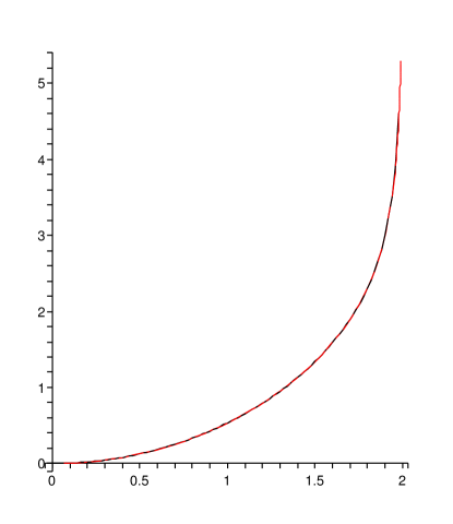
Figure 1: Lower bound on $\mathrm{KL}(P,Q)$ as a function of the variational divergence $V(P,Q)$. Both the explicit bound (4) and Fedotorev et al.’s implicit bound (2) are plotted.

4 Proof of Main Result

Proof  (Theorem 6) This proof is driven by the duality between the family of variational divergences $V_{\pi}(P,Q)$ and the 0-1 Bayes risk $\underline{\mathbb{L}}(\pi,P,Q)$ given in Lemma 3. Given distributions $P$ and $Q$ let

$$\phi(\pi)=V_{\pi}(P,Q)=\pi\wedge(1-\pi)-\psi(\pi),$$

where $\psi(\pi)=\underline{\mathbb{L}}(\pi,P,Q)$. We know that $\psi$ is non-negative and concave and satisfies $\psi(\pi)\leq\pi\wedge(1-\pi)$ and thus $\psi(0)=\psi(1)=0$.

Since

$$\mathbb{I}_{f}(P,Q)=\int_{0}^{1}\phi(\pi)\gamma_{f}(\pi)d\pi,$$ (25)

$\mathbb{I}_{f}(P,Q)$ is minimised by minimising $\phi$ over all $(P,Q)$ such that

$$\phi(\pi_{i})=\phi_{i}=\pi_{i}\wedge(1-\pi_{i})-\psi(\pi_{i}).$$

Since $\psi_{i}:=(1-\pi_{i})\wedge\pi_{i}-V_{\pi_{i}}(P,Q)=\psi(\pi_{i})$ the minimisation problem for $\phi$ can be expressed in terms of $\psi$ as:

$$\mbox{Given\ }(\pi_{i},\psi_{i})_{i=1}^{n} \mbox{find the maximal\ }\psi\!\colon\![0,1]\rightarrow[0,{\textstyle\frac{1}{2}}]$$ (26)

such that $$\psi(\pi_{i})=\psi_{i},\ \ i=0,\ldots,n+1,$$ (29)

$$\psi(\pi)\leq\pi\wedge(1-\pi),\ \ \pi\in[0,1],$$

$$\psi\mbox{\ is concave}.$$

This will tell us the optimal $\phi$ to use since optimising over $\psi$ is equivalent to optimising over $\underline{\mathbb{L}}(\cdot,P,Q)$. Under the additional assumption on $\mathcal{X}$, Corollary 5 implies that for any $\psi$ satisfying (29), (29) and (29) there exists $P,Q$ such that $\underline{\mathbb{L}}(\cdot,P,Q)=\psi(\cdot)$. This establishes the tightness of our bounds.

Let $\Psi$ be the set of piece-wise linear concave functions on $[0,1]$ having $n+1$ segments such that $\psi\in\Psi\Rightarrow\psi$ satisfies (29) and (29). We now show that in order to solve (26) it suffices to consider $\psi\in\Psi$.

If $g$ is a concave function on $\mathbb{R}$, then let

$$\eth g(x):=\{s\in\mathbb{R}\colon g(y)\leq g(x)+\langle s,y-x\rangle,\ y\in\mathbb{R}\}$$

denote the sup-differential of $g$ at $x$. (This is the obvious analogue of the sub-differential for convex functions (Rockafellar:1970, ).) Suppose $\tilde{\psi}$ is a general concave function satisfying (29) and (29). For $i=1,\ldots,n$, let

$$G_{i}^{\tilde{\psi}}:=\left\{[0,1]\ni g_{i}^{\tilde{\psi}}:\pi_{i}\mapsto\psi_{i}\in\mathbb{R}\ \ \mbox{is linear and}\right.$$

$$\ \ \ \ \ \ \ \textstyle\left.\left.\frac{\partial}{\partial\pi}g_{i}^{\tilde{\psi}}(\pi)\right|_{\pi=\pi_{i}}\in\eth\tilde{\psi}(\pi_{i})\right\}.$$

Observe that by concavity, for all concave $\tilde{\psi}$ satisfying (29) and (29), for all $g\in\bigcup_{i=1}^{n}G_{i}^{\tilde{\psi}}$, $g(\pi)\geq\psi(\pi)$, for $\pi\in[0,1]$.

Thus given any such $\tilde{\psi}$, one can always construct

$$\psi^{*}(\pi)=\min(g_{1}^{\tilde{\psi}}(\pi),\ldots,g_{n}^{\tilde{\psi}}(\pi))$$ (30)

such that $\psi^{*}$ is concave, satisfies (29) and $\psi^{*}(\pi)\geq\tilde{\psi}(\pi)$, for all $\pi\in[0,1]$. It remains to take account of (29). That is trivially done by setting

$$\psi(\pi)=\min(\psi^{*}(\pi),\pi\wedge(1-\pi))$$ (31)

which remains concave and piecewise linear (although with potentially one additional linear segment). Finally, the pointwise smallest concave $\psi$ satisfying (29) and (29) is the piecewise linear function connecting the points $(0,0),(\pi_{1},\psi_{1}),(\pi_{2},\psi_{2}),\ldots,(\pi_{m},\psi_{m}),(1,0)$.

Let $g\colon[0,1]\rightarrow[0,\frac{1}{2}]$ be this function which can be written explicitly as

$$g(\pi)=\left(\psi_{i}+\frac{(\psi_{i+1}-\psi)(\pi-\pi_{i})}{\pi_{i+1}-\pi_{i}}\right)\cdot\llbracket\pi\in[\pi_{i},\pi_{i+1}]\rrbracket,$$

where we have defined $\pi_{0}:=0$, $\psi_{0}:=0$, $\pi_{n+1}:=1$ and $\psi_{n+1}:=0$.

We now explicitly parametrize this family of functions. Let $p_{i}\colon[0,1]\rightarrow\mathbb{R}$ denote the affine segment the graph of which passes through $(\pi_{i},\psi_{i})$, $i=0,\ldots,n+1$. Write $p_{i}(\pi)=a_{i}\pi+b_{i}$. We know that $p_{i}(\pi_{i})=\psi_{i}$ and thus

$$b_{i}=\psi_{i}-a_{i}\pi_{i},\ \ \ i=0,\ldots,n+1.$$ (32)

In order to determine the constraints on $a_{i}$, since $g$ is concave and minorizes $\psi$, it suffices to only consider $(\pi_{i-1},g(\pi_{i-1}))$ and $(\pi_{i+1},g(\pi_{i+1}))$ for $i=1,\ldots,n$. We have (for $i=1,\ldots,n$)

$$p_{i}(\pi_{i-1}) \geq g(\pi_{i-1})$$

$$\Rightarrow a_{i}\pi_{i-1}+b_{i} \geq\psi_{i-1}$$

$$\Rightarrow a_{i}\pi_{i-1}+\psi_{i}-a_{i}\pi_{i} \geq\psi_{i-1}$$

$$\Rightarrow a_{i}\underbrace{(\pi_{i-1}-\pi_{i})}_{<0} \geq\psi_{i-1}-\psi_{i}$$

$$\Rightarrow a_{i} \leq\frac{\psi_{i-1}-\psi_{i}}{\pi_{i-1}-\pi_{i}}.$$ (33)

Similarly we have (for $i=1,\ldots,n$)

$$p_{i}(\pi_{i+1}) \geq g(\pi_{i+1})$$

$$\Rightarrow a_{i}\pi_{i+1}+b_{i} \geq\psi_{i+1}$$

$$\Rightarrow a_{i}\pi_{i+1}+\psi_{i}-a_{i}\pi_{i} \geq\psi_{i+1}$$

$$\Rightarrow a_{i}\underbrace{(\pi_{i+1}-\pi_{i})}_{>0} \geq\psi_{i+1}-\psi_{i}$$

$$\Rightarrow a_{i} \geq\frac{\psi_{i+1}-\psi_{i}}{\pi_{i+1}-\pi_{i}}.$$ (34)

We now determine the points at which $\psi$ defined by (30) and (31) change slope. That occurs at the points $\pi$ when

$$p_{i}(\pi) =p_{i+1}(\pi)$$

$$\Rightarrow a_{i}\pi+\psi_{i}-a_{i}\pi_{i} =a_{i+1}\pi+\psi_{i+1}-a_{i+1}\pi_{i+1}$$

$$\Rightarrow (a_{i+1}-a_{i})\pi =\psi_{i}-\psi_{i+1}+a_{i+1}\pi_{i+1}-a_{i}\pi_{i}$$

$$\Rightarrow \pi =\frac{\psi_{i}-\psi_{i+1}+a_{i+1}\pi_{i+1}}{a_{i+1}-a_{i}}$$

$$=:\tilde{\pi}_{i}$$

for $i=0,\ldots,n$. Thus

$$\psi(\pi)=p_{i}(\pi),\ \ \ \pi\in[\tilde{\pi}_{i-1},\tilde{\pi}_{i}],\ i=1,\ldots,n.$$

Let $\mathbf{a}=(a_{1},\ldots,a_{n})$. We explicitly denote the dependence of $\psi$ on $\mathbf{a}$ by writing $\psi_{\mathbf{a}}$. Let

$$\phi_{\mathbf{a}}(\pi) := \pi\wedge(1-\pi)-\psi_{\mathbf{a}}(\pi)$$

$$= \alpha_{\mathbf{a},i}\pi+\beta_{\mathbf{a},i},\ \pi\in[\bar{\pi}_{i-1},\bar{\pi}_{i}],i=1,\ldots,n+1,$$

where $\mathbf{a}\in A_{n}$ (see (6)), $\bar{\pi}_{i}$, $\alpha_{\mathbf{a},i}$ and $\beta_{\mathbf{a},i}$ are defined by (18), (19) and (20) respectively. The extra segment induced at index $j$ (see (17)) is needed since $\pi\mapsto\pi\wedge(1-\pi)$ has a slope change at $\pi={\textstyle\frac{1}{2}}$. Thus in general, $\phi_{\mathbf{a}}$ is piece-wise linear with $n+2$ segments (recall $i$ ranges from $0$ to $n+2$); if $\tilde{\pi}_{k+1}=\frac{1}{2}$ for some $k\in\{1,\ldots,n\}$, then there will be only $n+1$ non-trivial segments.

Thus

$$\left\{\pi\mapsto\sum_{i=0}^{n}\phi_{\mathbf{a}}(\pi)\cdot\llbracket\pi\in[\bar{\pi}_{i},\bar{\pi}_{i+1}]\rrbracket\colon\mathbf{a}\in A_{n}\right\}$$

is the set of $\phi$ consistent with the constraints and $A_{n}$ is defined in (6). Thus substituting into (25), interchanging the order of summation and integration and optimizing we have shown (23). The tightness has already been argued: under the additional assumption on $\mathcal{X}$, since there is no slop in the argument above since every $\psi$ satisfying the constraints in (26) is the Bayes risk function for some $(P,Q)$.  

Proof  (Theorem 7) In this case $n=1$ and the optimal $\psi$ function will be piecewise linear, concave, and its graph will pass through $(\pi_{1},\psi_{1})$. Thus the optimal $\phi$ will be of the form

$$\phi(\pi)=\left\{\begin{array}[]{ll}0,&\pi\in[0,L]\cup[U,1]\\ \pi-(a\pi+b),&\pi\in[L,{\textstyle\frac{1}{2}}]\\ (1-\pi)-(a\pi+b),&\pi\in[{\textstyle\frac{1}{2}},U].\end{array}\right.$$

where $a\pi_{1}+b=\psi_{1}\Rightarrow b=\psi_{1}-a\pi_{1}$ and $a\in[-2\psi_{1},2\psi_{1}]$ (see Figure 3).

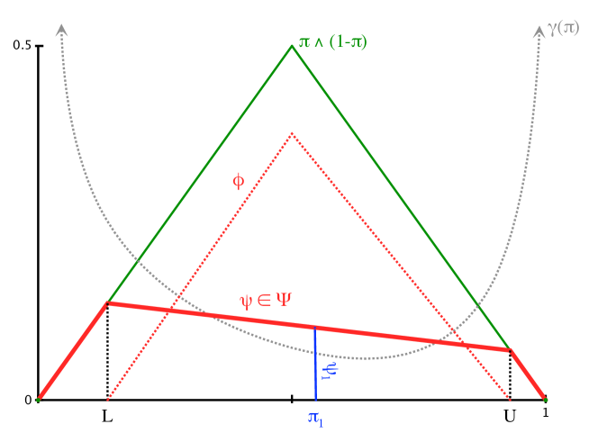
Figure 3: The optimisation problem when $n=1$. Given $\psi_{1}$, there are many risk curves consistent with it. The optimisation problem involves finding the piece-wise linear concave risk curve $\psi\in\Psi$ and the corresponding $\phi=\pi\wedge(1-\pi)-\psi$ that maximises $\mathbb{I}_{f}$. $L$ and $U$ are defined in the text.

For variational divergence, $\pi_{1}={\textstyle\frac{1}{2}}$ and thus by (11)

$$\psi_{1}=\pi_{1}\wedge(1-\pi_{1})-\frac{V}{4}=\frac{1}{2}-\frac{V}{4}$$ (35)

and so $\phi_{1}=V/4$. We can thus determine $L$ and $U$:

$$aL+b =L$$

$$\Rightarrow aL+\psi_{1}-a\pi_{1} =L$$

$$\Rightarrow L =\frac{a\pi_{1}-\psi_{1}}{a-1}.$$

Similarly $aU+b=1-U\Rightarrow U=\frac{1-\psi_{1}+a\pi_{1}}{a+1}$ and thus

$$\mathbb{I}_{f}(P,Q)\geq\!\!\!\min_{a\in[-2\psi_{1},2\psi_{1}]}\!\!\!\int\limits_{\frac{a\pi_{1}-\psi_{1}}{a-1}}^{\frac{1}{2}}\!\!\!\!\![(1-a)\pi-\psi_{1}+a\pi_{1}]\gamma_{f}(\pi)d\pi$$

$$\ \ \ \ +\int\limits_{\frac{1}{2}}^{\frac{1-\psi_{1}+a\pi_{1}}{a+1}}\!\!\!\!\![(-a-1)\pi-\psi_{1}+a\pi_{1}+1]\gamma_{f}(\pi)d\pi.$$ (36)

If $\gamma_{f}$ is symmetric about $\pi={\textstyle\frac{1}{2}}$ and convex and $\pi_{1}={\textstyle\frac{1}{2}}$, then the optimal $a=0$. Thus in that case,

$$\mathbb{I}_{f}(P,Q) \geq 2\int_{\psi_{1}}^{\frac{1}{2}}(\pi-\psi_{1})\gamma_{f}(\pi)d\pi$$

$$= 2\left[({\textstyle\frac{1}{2}}-\psi_{1})\Gamma_{f}({\textstyle\frac{1}{2}})+\bar{\Gamma}_{f}(\psi_{1})-\bar{\Gamma}_{f}({\textstyle\frac{1}{2}})\right]$$

$$= 2\left[\textstyle\frac{V}{4}\Gamma_{f}({\textstyle\frac{1}{2}})+\bar{\Gamma}_{f}\left({\textstyle\frac{1}{2}}-\textstyle\frac{V}{4}\right)-\bar{\Gamma}_{f}({\textstyle\frac{1}{2}})\right].$$ (38)

Combining the above with (35) leads to a range of Pinsker style bounds for symmetric $\mathbb{I}_{f}$:

Jeffrey’s Divergence

Since $J(P,Q)=\mathrm{KL}(P,Q)+\mathrm{KL}(Q,P)$ we have $\gamma(\pi)=\frac{1}{\pi^{2}(1-\pi)^{2}}$. (As a check, $f(t)=(t-1)\ln(t)$, $f^{\prime\prime}(t)=\frac{t+1}{t^{2}}$ and so $\gamma_{f}(\pi)=\frac{1}{\pi^{3}}f^{\prime\prime}\left(\frac{1-\pi}{\pi}\right)=\frac{1}{\pi^{2}(1-\pi)^{2}}$.) Thus

$$J(P,Q) \geq 2\int_{\psi_{1}}^{1/2}\frac{(\pi-\psi_{1})}{\pi^{2}(1-\pi)^{2}}d\pi$$

$$= (4\psi_{1}-2)(\ln(\psi_{1})-\ln(1-\psi_{1})).$$

Substituting $\psi_{1}=\frac{1}{2}-\frac{V}{4}$ gives

$$J(P,Q)\geq V\ln\left(\frac{2+V}{2-V}\right).$$

Observe that the above bound behaves like $V^{2}$ for small $V$, and $V\ln\left(\frac{2+V}{2-V}\right)\geq V^{2}$ for $V\in[0,2]$. Using the traditional Pinkser inequality ($\mathrm{KL}(P,Q)\geq V^{2}/2$) we have

$$J(P,Q) = \mathrm{KL}(P,Q)+\mathrm{KL}(Q,P)$$

$$\geq \frac{V^{2}}{2}+\frac{V^{2}}{2}=V^{2}.$$

Jensen-Shannon Divergence

Here $f(t)=\frac{t}{2}\ln t-\frac{(t+1)}{2}\ln(t+1)+\ln 2$ and thus $\gamma_{f}(\pi)=\frac{1}{\pi^{3}}f^{\prime\prime}\left(\frac{1-\pi}{\pi}\right)=\frac{1}{2\pi(1-\pi)}$. Thus

$$I(P,Q) = 2\int_{\psi_{1}}^{\frac{1}{2}}\frac{\pi-\psi_{1}}{2\pi(1-\pi)}d\pi$$

$$= \ln(1\!-\!\psi_{1})-\psi_{1}\ln(1\!-\!\psi_{1})+\psi_{1}\ln\psi_{1}+\ln(2).$$

Substituting $\psi_{1}=\frac{1}{2}-\frac{V}{4}$ leads to

$$I(P,Q)\geq\left(\textstyle\frac{1}{2}-\textstyle\frac{V}{4}\right)\ln(2-V)+\left(\textstyle\frac{1}{2}+\textstyle\frac{V}{4}\right)\ln(2+V)-\ln(2).$$

Hellinger Divergence

Here $f(t)=(\sqrt{t}-1)^{2}$. Consequently $\gamma_{f}(\pi)=\frac{1}{\pi^{3}}f^{\prime\prime}\left(\frac{1-\pi}{\pi}\right)=\frac{1}{\pi^{3}}\frac{1}{2\left((1-\pi)/\pi\right)^{3/2}}=\frac{1}{2[\pi(1-\pi)]^{3/2}}$ and thus

$$h^{2}(P,Q) \geq 2\int_{\psi_{1}}^{\frac{1}{2}}\frac{\pi-\psi_{1}}{2[\pi(1-\pi)]^{3/2}}d\pi$$

$$= \frac{4\sqrt{\psi_{1}}(\psi_{1}-1)+2\sqrt{1-\psi_{1}}}{\sqrt{1-\psi_{1}}}$$

$$= \frac{4\sqrt{\frac{1}{2}-\frac{V}{4}}\left(\frac{1}{2}-\frac{V}{4}-1\right)+2\sqrt{1-\frac{1}{2}+\frac{V}{4}}}{\sqrt{1-\frac{1}{2}+\frac{V}{4}}}$$

$$= 2-\frac{(2+V)\sqrt{2-V}}{\sqrt{2+V}}$$

$$= 2-\sqrt{4-V^{2}}.$$

For small $V$, $2-\sqrt{4-V^{2}}\approx V^{2}/4$.

Arithmetic-Geometric Mean Divergence

In this case, $f(t)=\frac{t+1}{2}\ln\left(\frac{t+1}{2\sqrt{t}}\right)$. Thus $f^{\prime\prime}(t)=\frac{t^{2}+1}{4t^{2}(t+1)}$ and hence $\gamma_{f}(\pi)=\frac{1}{\pi^{3}}f^{\prime\prime}\left(\frac{1-\pi}{\pi}\right)=\gamma_{f}(\pi)=\frac{2\pi^{2}-2\pi+1}{\pi^{2}(\pi-1)^{2}}$ and thus

$$T(P,Q) \geq 2\int_{\psi_{1}}^{\frac{1}{2}}(\pi-\psi_{1})\frac{2\pi^{2}-2\pi+1}{\pi^{2}(\pi-1)^{2}}d\pi$$

$$= -\frac{1}{2}\ln(1-\psi)-\frac{1}{2}\ln(\psi)-\ln(2).$$

Substituting $\psi_{1}=\frac{1}{2}-\frac{V}{4}$ gives

$$T(P,Q) \geq -\frac{1}{2}\ln\left(\frac{1}{2}+\frac{V}{4}\right)-\frac{1}{2}\ln\left(\frac{1}{2}-\frac{V}{4}\right)-\ln(2)$$

$$= \ln\left(\frac{4}{\sqrt{4-V^{2}}}\right)-\ln(2).$$

Symmetric $\chi^{2}$-Divergence

In this case $\Psi(P,Q)=\chi^{2}(P,Q)+\chi^{2}(Q,P)$ and thus (see below) $\gamma_{f}(\pi)=\frac{2}{\pi^{3}}+\frac{2}{(1-\pi)^{3}}$. (As a check, from $f(t)=\frac{(t-1)^{2}(t+1)}{t}$ we have $f^{\prime\prime}(t)=\frac{2(t^{3}+1)}{t^{3}}$ and thus $\gamma_{f}(\pi)=\frac{1}{\pi^{3}}f^{\prime\prime}\left(\frac{1-\pi}{\pi}\right)$ gives the same result.)

$$\Psi(P,Q) \geq 2\int_{\psi_{1}}^{\frac{1}{2}}(\pi-\psi_{1})\left(\frac{2}{\pi^{3}}+\frac{2}{(1-\pi)^{3}}\right)d\pi$$

$$= \frac{2(1+4\psi_{1}^{2}-4\psi_{1})}{\psi_{1}(\psi_{1}-1)}.$$

Substituting $\psi_{1}=\frac{1}{2}-\frac{V}{4}$ gives $\Psi(P,Q)\geq\frac{8V^{2}}{4-V^{2}}$.

When $\gamma_{f}$ is not symmetric, one needs to use (36) instead of the simpler (38). We consider two cases.

$\chi^{2}$-Divergence

Here $f(t)=(t-1)^{2}$ and so $f^{\prime\prime}(t)=2$ and hence $\gamma(\pi)=f^{\prime\prime}\left(\frac{1-\pi}{\pi}\right)/\pi^{3}=\frac{2}{\pi^{3}}$ which is not symmetric. Upon substituting $2/\pi^{3}$ for $\gamma(\pi)$ in (36) and evaluating the integrals we obtain

$$\chi^{2}(P,Q)\geq 2\min_{a\in[-2\psi_{1},2\psi_{1}]}\underbrace{\textstyle\frac{1+4\psi_{1}^{2}-4\psi_{1}}{2\psi_{1}-a}-\frac{1+4\psi_{1}^{2}-4\psi_{1}}{2\psi_{1}-a-2}}_{=:J(a,\psi_{1})}.$$

One can then solve $\frac{\partial}{\partial a}J(a,\psi_{1})=0$ for $a$ and one obtains $a^{*}=2\psi_{1}-1$. Now $a^{*}>-2\psi_{1}$ only if $\psi_{1}>\frac{1}{4}$. One can check that when $\psi_{1}\leq\frac{1}{4}$, then $a\mapsto J(a,\psi_{1})$ is monotonically increasing for $a\in[-2\psi_{1},2\psi_{1}]$ and hence the minimum occurs at $a^{*}=-2\psi_{1}$. Thus the value of $a$ minimising $J(a,\psi_{1})$ is

$$a^{*}=\llbracket\psi_{1}>1/4\rrbracket(2\psi_{1}-1)+\llbracket\psi_{1}\leq 1/4\rrbracket(-2\psi_{1}).$$

Substituting the optimal value of $a^{*}$ into $J(a,\psi_{1})$ we obtain

$$J(a^{*},\psi_{1}) = \llbracket\psi_{1}>1/4\rrbracket(2+8\psi_{1}^{2}-8\psi_{1})$$

$$+\llbracket\psi_{1}\leq 1/4\rrbracket\left(\frac{1+4\psi_{1}^{2}-4\psi}{4\psi}-\frac{1+4\psi_{1}^{2}-4\psi}{4\psi_{1}-2}\right).$$

Substituting $\psi_{1}=\frac{1}{2}-\frac{V}{4}$ and observing that $V<1\Rightarrow\psi_{1}>1/4$ we obtain

$$\chi^{2}(P,Q)\geq\llbracket V<1\rrbracket V^{2}+\llbracket V\geq 1\rrbracket\frac{V}{(2-V)}.$$

Observe that the bound diverges to $\infty$ as $V\rightarrow 2$.

Kullback-Leibler Divergence

In this case we have $f(t)=t\ln t$ and thus $f^{\prime\prime}(t)=1/t$ and consequently $\gamma_{f}(\pi)=\frac{1}{\pi^{3}}f^{\prime\prime}\left(\frac{1-\pi}{\pi}\right)=\frac{1}{\pi^{2}(1-\pi)}$ which is clearly not symmetric. From (36) we obtain

$$\mathrm{KL}(P,Q)\geq\min_{[-2\psi_{1},2\psi_{1}]}\left(1-\textstyle\frac{a}{2}-\psi_{1}\right)\ln\left(\textstyle\frac{a+2\psi_{1}-2}{a-2\psi_{1}}\right)$$

$$\ \ \ \ \ \ \ +\left(\textstyle\frac{a}{2}+\psi_{1}\right)\ln\left(\textstyle\frac{a+2\psi_{1}}{a-2\psi_{1}+2}\right).$$

Substituting $\psi_{1}=\frac{1}{2}-\frac{V}{4}$ gives

$$\mathrm{KL}(P,Q)\geq\min_{a\in\left[\frac{V-2}{2},\frac{2-V}{2}\right]}\delta_{a}(V),$$

where

$$\delta_{a}(V)\!=\!\textstyle\left(\frac{V+2-2a}{4}\right)\ln\left(\frac{2a-2-V}{2a-2+V}\right)+\left(\frac{2a+2-V}{4}\right)\ln\left(\frac{2a+2-V}{2a+2+V}\right).$$

Set $\beta:=2a$ and we have (4).  

5 Conclusion

We have generalised the classical Pinsker inequality and developed best possible bounds for the general situation. A special case of the result gives an explicit bound relating Kullback-Liebler divergence and variational divergence. The proof relied on an integral representation of $f$-divergences in terms of statistical information. Such representations are a powerful device as they identify the primitives underpinning general learning problems. These representations are further studied in ReidWilliamson2009 .

Appendix A History of Pinsker Inequalities

Pinsker Pinsker1964 presented the first bound relating $\mathrm{KL}(P,Q)$ to $V(P,Q)$: $\mathrm{KL}\geq V^{2}/2$ and it is now known by his name or sometimes as the Pinsker-Csiszár-Kullback inequality since Csiszar Csiszar1967 presented another version and Kullback Kullback1967 showed $\mathrm{KL}\geq V^{2}/2+V^{4}/36$. Much later Topsøe Topsoe2001 showed $\mathrm{KL}\geq V^{2}/2+V^{4}/36+V^{6}/270$. Non-polynomial bounds are due to Vajda Vajda1970 : $\mathrm{KL}\geq L_{\mathrm{Vajda}}(V):=\log\left(\frac{2+V}{2-V}\right)-\frac{2V}{2+V}$ and Toussaint Toussaint1978 who showed $\mathrm{KL}\geq L_{\mathrm{Vajda}}(V)\vee(V^{2}/2+V^{4}/36+V^{8}/288)$.

Care needs to be taken when comparing results from the literature as different definitions for the divergences exist. For example Gibbs and Su GibbsSu2002 used a definition of $V$ that differs by a factor of 2 from ours. There are some isolated bounds relating $V$ to some other divergences, analogous to the classical Pinkser bound; Kumar Kumar2005 has presented a summary as well as new bounds for a wide range of symmetric $f$-divergences by making assumptions on the likelihood ratio: $r\leq p(x)/q(x)\leq R<\infty$ for all $x\in\mathcal{X}$. This line of reasoning has also been developed by Dragomir et al. DragomirGluvsvcevicPearce2001 and Taneja Taneja2005 ; Taneja2005a . Topsøe Topsoe:2000 has presented some infinite series representations for capacitory discrimination in terms of triangular discrimination which lead to inequalities between those two divergences. Liese and Miescke (Liese2008, , p.48) give the inequality $V\leq h\sqrt{4-h^{2}}$ (which seems to be originally due to LeCam LeCam1986 ) which when rearranged corresponds exactly to the bound for $h^{2}$ in theorem 7. Withers Withers1999 has also presented some inequalities between other (particular) pairs of divergences; his reasoning is also in terms of infinite series expansions.

Arnold et al. ArnoldMarkowichToscaniUnterreiter considered the case of $n=1$ but arbitrary $\mathbb{I}_{f}$ (that is they bound an arbitrary $f$-divergence in terms of the variational divergence). Their argument is similar to the geometric proof of Theorem 6. They do not compute any of the explicit bounds in theorem 7 except they state (page 243) $\chi^{2}(P,Q)\geq V^{2}$ which is looser than (3).

Gilardoni Gilardoni:2006 showed (via an intricate argument) that if $f^{\prime\prime\prime}(1)$ exists, then $\mathbb{I}_{f}\geq\frac{f^{\prime\prime}(1)V^{2}}{2}$. He also showed some fourth order inequalities of the form $\mathbb{I}_{f}\geq c_{2,f}V^{2}+c_{4,f}V^{4}$ where the constants depend on the behaviour of $f$ at 1 in a complex way. Gilardoni Gilardoni2006 ; Gilardoni2006a presented a completely different approach which obtains many of the results of theorem 7. Gilardoni Gilardoni2006a improved Vajda’s bound slightly to $\mathrm{KL}(P,Q)\geq\ln\frac{2}{2-V}-\frac{2-V}{2}\ln\frac{2+V}{2}$.

Gilardoni Gilardoni2006 ; Gilardoni2006a presented a general tight lower bound for $\mathbb{I}_{f}=\mathbb{I}_{f}(P,Q)$ in terms of $V=V(P,Q)$ which is difficult to evaluate explicitly in general:

$$\mathbb{I}_{f}\geq\frac{V}{2}\left(\frac{f[g_{R}^{-1}(k(1/V))]}{g_{R}^{-1}(k(1/V))-1}+\frac{f[g_{L}^{-1}(k(1/V))]}{1-g_{L}^{-1}(k(1/V))}\right),$$

where $k^{-1}(t)=\frac{1}{2}\left(\frac{1}{1-g_{L}^{-1}(t)}+\frac{1}{g_{R}^{-1}(t)-1}\right)$ and of course $k(u)=(k^{-1})^{-1}(u)$; and $g(u)=(u-1)f^{\prime}(u)-f(u)$, $g_{R}^{-1}[g(u)]=u$ for $u\geq 1$ and $g_{L}^{-1}[g(u)]=u$ for $u\leq 1$. He presented a new parametric form for $\mathbb{I}_{f}=\mathrm{KL}$ in terms of Lambert’s $W$ function. In general, the result is analogous to that of Fedotov et al. FedotovTopsoe2003 in that it is in a parametric form which, if one wishes to evaluate for a particular $V$, one needs to do a one dimensional numerical search — as complex as (4). However, when $f$ is such that $\mathbb{I}_{f}$ is symmetric, this simplifies to the elegant form $\mathbb{I}_{f}\geq\frac{2-V}{2}f\left(\frac{2+V}{2-V}\right)-f^{\prime}(1)V$. He presented explicit special cases for $h^{2}$, $J$,$\Delta$ and $I$ identical to the results in Theorem 7. It is not apparent how the approach of Gilardoni Gilardoni2006 ; Gilardoni2006a could be extended to more general situations such as that in Theorem 6 (i.e. $n>1$).

Bolley and Villani BolleyVillani2005 considered weighted versions of the Pinsker inequalities (for a weighted generalisation of Variational divergence) in terms of KL-divergence that are related to transportation inequalities.

Acknowledgements

This work was supported by the Australian Research Council and NICTA; an initiative of the Commonwealth Government under Backing Australia’s Ability.

References

- [1] S.M. Ali and S.D. Silvey. A general class of coefficients of divergence of one distribution from another. Journal of the Royal Statistical Society. Series B (Methodological), 28(1):131–142, 1966.
- [2] F. Bolley and C. Villani. Weighted Csiszár-Kullback-Pinsker inequalities and applications to transportation inequalities. Annales de la Faculte des Sciences de Toulouse, 14(3):331–352, 2005.
- [3] I. Csiszár. Information-type measures of difference of probability distributions and indirect observations. Studia Scientiarum Mathematicarum Hungarica, 2:299–318, 1967.
- [4] M.H. DeGroot. Uncertainty, Information, and Sequential Experiments. The Annals of Mathematical Statistics, 33(2):404–419, 1962.
- [5] Luc Devroye, László Györfi, and Gábor Lugosi. A Probabilistic Approach to Pattern Recognition. Springer, New York, 1996.
- [6] S.S. Dragomir, V. Gluščević, and C.E.M. Pearce. Csiszár -divergence, Ostrowski’s inequality and mutual information. Nonlinear Analysis, 47:2375–2386, 2001.
- [7] A.A. Fedotov, P. Harremoës, and F. Topsøe. Refinements of Pinsker’s inequality. IEEE Transactions on Information Theory, 49(6):1491–1498, June 2003.
- [8] Alison L. Gibbs and Francis Edward Su. On choosing and bounding probability metrics. International Statistical Review, 70:419–435, 2002.
- [9] G. L. Gilardoni. On Pinsker’s Type Inequalities and Csiszár’s -divergences. Part I: Second and Fourth-Order Inequalities. arXiv:cs/0603097v2, April 2006.
- [10] Gustavo L. Gilardoni. On the minimum -divergence for a given total variation. Comptes Rendus Académie des sciences, Paris, Series 1, 343, 2006.
- [11] Gustavo L. Gilardoni. On the relationship between symmetric -divergence and total variation and an improved Vajda’s inequality. Preprint, Departamento de Estatística, Universidade de Brasília, April 2006.
- [12] Cornelius Gutenbrunner. On applications of the representation of -divergences as averaged minimal Bayesian risk. In Transactions of the 11th Prague Conference on Information Theory, Statistical Decision Functions and Random Processes, pages 449–456, Dordrecht; Boston, 1990. Kluwer Academic Publishers.
- [13] Mohammadali Khosravifard, Dariush Fooladivanda, and T. Aaron Gulliver. Confliction of the Convexity and Metric Properties in -Divergences. IEICE Transactions on Fundamentals of Electronics, Communication and Computer Sciences, E90-A(9):1848–1853, 2007.
- [14] S. Kullback. Lower bound for discrimination information in terms of variation. IEEE Transactions on Information Theory, 13:126–127, 1967. Correction, volume 16, p. 652, September 1970.
- [15] P. Kumar and S. Chhina. A symmetric information divergence measure of the Csiszár’s -divergence class and its bounds. Computers and Mathematics with Applications, 49:575–588, 2005.
- [16] Lucien LeCam. Asymptotic Methods in Statistical Decision Theory. Springer, 1986.
- [17] F. Liese and I. Vajda. On divergences and informations in statistics and information theory. IEEE Transactions on Information Theory, 52(10):4394–4412, 2006.
- [18] Friedrich Liese and Klaus-J. Miescke. Statistical Decision Theory. Springer, New York, 2008.
- [19] X. Nguyen, M.J. Wainwright, and M.I. Jordan. On distance measures, surrogate loss functions, and distributed detection. Technical Report 695, Department of Statistics, University of California, Berkeley, October 2005.
- [20] F. Österreicher and I. Vajda. Statistical information and discrimination. IEEE Transactions on Information Theory, 39(3):1036–1039, 1993.
- [21] M.S. Pinsker. Information and Information Stability of Random Variables and Processes. Holden-Day, 1964.
- [22] Mark D. Reid and Robert C. Williamson. Information, divergence and risk for binary experiments. arXiv preprint arXiv:0901.0356v1, January 2009.
- [23] R. T. Rockafellar. Convex Analysis. Princeton Landmarks in Mathematics and Physics. Princeton University Press, 1970.
- [24] I.J. Taneja. Bounds on non-symmetric divergence measures in terms of symmetric divergence measures. arXiv:math.PR/0506256v1, 2005.
- [25] I.J. Taneja. Refinement inequalities among symmetric divergence measures. arXiv:math/0501303v2, April 2005.
- [26] F. Topsøe. Bounds for entropy and divergence for distributions over a two-element set. J. Ineq. Pure & Appl. Math, 2(2), 2001.
- [27] Flemming Topsøe. Some inequalities for information divergence and related measures of discrimination. IEEE Transactions on Information Theory, 46(4):1602–1609, 2000.
- [28] E.N. Torgersen. Comparison of Statistical Experiments. Cambridge University Press, 1991.
- [29] G.T. Toussaint. Probability of error, expected divergence and the affinity of several distributions. IEEE Transactions on Systems, Man and Cybernetics, 8:482–485, 1978.
- [30] Andreas Unterreiter, Anton Arnold, Peter Markowich, and Giuseppe Toscani. On generalized Csiszár-Kullback inequalities. Monatshefte für Mathematik, 131:235–253, 2000.
- [31] I. Vajda. Note on discrimination and variation. IEEE Transactions on Information Theory, 16:771–773, 1970.
- [32] Lang Withers. Some inequalities relating different measures of divergence between two probability distributions. IEEE Transactions on Information Theory, 45(5):1728–1735, 1999.