Feshbach Resonance in Optical Lattices and the Quantum Ising Model

Abstract

Motivated by experiments on heteronuclear Feshbach resonances in Bose mixtures, we investigate $s$-wave pairing of two species of bosons in an optical lattice. The zero temperature phase diagram supports a rich array of superfluid and Mott phases and a network of quantum critical points. This topology reveals an underlying structure that is succinctly captured by a two-component Landau theory. Within the second Mott lobe we establish a quantum phase transition described by the paradigmatic longitudinal and transverse field Ising model. This is confirmed by exact diagonalization of the 1D bosonic Hamiltonian. We also find this transition in the homonuclear case.

Introduction.— With the advent of ultra-cold atomic gases, the fermionic BEC–BCS crossover has been the focus of intense scrutiny Donley et al. (2002); Regal et al. (2003, 2004). Tremendous experimental control has been achieved through the use of Feshbach resonances, which allow one to manipulate atomic interactions by a magnetic field. By sweeping the strength of attraction, one may interpolate between a BEC of tightly bound molecules, and a BCS state of loosely associated pairs. More recently, the analogous problem for a single species of boson has been the subject of theoretical investigation Radzihovsky et al. (2004); Romans et al. (2004); Koetsier et al. (2009); Radzihovsky et al. (2008); Rousseau and Denteneer (2009, 2008). An important distinction from the fermionic case is that the carriers themselves may condense. This leads to the possibility of novel phases and phase transitions, with no fermionic counterpart.

In parallel, there has been a significant experimental drive to study Feshbach resonances in binary mixtures of different atomic species. An important catalyst is the quest for heteronuclear molecules as a route to dipolar interactions and exotic condensates Santos et al. (2000). Recently, heteronuclear molecules have been created in ${}^{85}{\rm Rb}$–${}^{87}{\rm Rb}$ bosonic mixtures through both s-wave Papp and Wieman (2006) and p-wave resonances Papp et al. (2008); Ticknor et al. (2004). Similarly, bosonic ${}^{41}{\rm K}$–${}^{87}{\rm Rb}$ mixtures have been studied in harmonic potentials Modugno et al. (2002) and in optical lattices Catani et al. (2008), and interspecies resonances have also been achieved Weber et al. (2008); Thalhammer et al. (2008, 2009). The enhanced longevity of molecules in optical lattices Thalhammer et al. (2006), and the sympathetic cooling of one species by the other, make these attractive for experiment. Multiple species also provide additional “isospin” degrees of freedom, and offer exciting possibilities for interesting phases and quantum magnetism Altman et al. (2003).

Motivated by these significant developments we consider the s-wave heteronuclear Feshbach problem for two-component bosons in an optical lattice. Our primary goal is to establish and explore the rich phase diagram, which supports distinct atomic and molecular superfluids in proximity to Mott phases. We also shed light on the nature of the quantum phase transitions, and a key finding is a transition described by the paradigmatic quantum Ising model. This ubiquitous model plays a central role in a variety of quantum many body contexts, and a controllable realization in cold atomic gases may open new directions on dynamics and frustrated lattices.

The Model.— Let us consider a two-component Bose gas with a “spin” index $\downarrow,\uparrow$. We assume that these components may form molecules, $m$. The Hamiltonian

$$H =\sum_{i\alpha}\epsilon_{\alpha}n_{i\alpha}-\sum_{\langle ij\rangle}\sum_{\alpha}t_{\alpha}\left(a_{i\alpha}^{\dagger}a_{j\alpha}+{\rm h.c.}\right)$$ (1)

$$\hskip 28.45274pt+\sum_{i\alpha\alpha^{\prime}}\frac{U_{\alpha\alpha^{\prime}}}{2}:n_{i\alpha}n_{i\alpha^{\prime}}:+\,H_{F},$$

describes bosons, $a_{i\alpha}$, hopping on a lattice with sites $i$, where $\alpha=\downarrow,\uparrow,m$ labels the carrier. Here, $\epsilon_{\alpha}$ are onsite potentials, $t_{\alpha}$ are hopping parameters, $\langle ij\rangle$ denotes summation over nearest neighbor bonds, and $U_{\alpha\alpha^{\prime}}$ are interactions. We assume that molecule formation is described by the s-wave interspecies Feshbach resonance term

$$H_{F}=g\sum_{i}(a^{\dagger}_{im}a_{i\uparrow}a_{i\downarrow}+{\rm h.c.}).$$ (2)

For recent work on the $p$-wave problem see Ref. Radzihovsky and Choi (2009). Normal ordering yields $:n_{i\alpha}n_{i\alpha}:=n_{i\alpha}(n_{i\alpha}-1)$ for like species, and $:n_{i\alpha}n_{i\alpha^{\prime}}:=n_{i\alpha}n_{i\alpha^{\prime}}$ for distinct species. To aid numerical simulations we consider hardcore atoms and molecules and set $U_{m\uparrow}=U_{m\downarrow}\equiv U$ and $U_{\uparrow\downarrow}\equiv V$. We work in the grand canonical ensemble with $H_{\mu}=H-\mu_{\rm T}N_{\rm T}-\mu_{\rm D}N_{\rm D}$, where $N_{\rm T}\equiv\sum_{i}(n_{i{\uparrow}}+n_{i\downarrow}+2n_{im})$ and $N_{\rm D}\equiv\sum_{i}(n_{i\uparrow}-n_{i\downarrow})$ commute with $H$. These are the total atom number (including a factor of two for molecules) and the up-down population imbalance respectively.

Phase Diagram.— To establish the phase diagram it is convenient to first examine the zero hopping limit. This helps constrain the overall topology and provides some orientation for the general problem. With three species of hardcore bosons we need to consider eight possible states in the occupation basis, $|n_{\downarrow},n_{\uparrow};n_{m}\rangle$. The Feshbach coupling, $g$, only mixes $|1,1;0\rangle$ and $|0,0;1\rangle$, and the resulting eigenstates $|\pm\rangle$ have energies $E_{\pm}=\tilde{\epsilon}_{m}-h/2\pm\sqrt{(h/2)^{2}+g^{2}}$, where $h\equiv\epsilon_{m}-\epsilon_{\downarrow}-\epsilon_{\uparrow}-V$ and the chemical potentials are absorbed into $\tilde{\epsilon}_{\uparrow}\equiv\epsilon_{\uparrow}-\mu_{\rm T}-\mu_{\rm D}$, $\tilde{\epsilon}_{\downarrow}\equiv\epsilon_{\downarrow}-\mu_{\rm T}+\mu_{\rm D}$, $\tilde{\epsilon}_{m}\equiv\epsilon_{m}-2\mu_{\rm T}$. The remaining six states have energies $E(n_{\downarrow},n_{\uparrow};n_{m})=\sum_{\alpha}\tilde{\epsilon}_{\alpha}n_{\alpha}+Vn_{\uparrow}n_{\downarrow}+Un_{m}(n_{\uparrow}+n_{\downarrow})$. Minimizing over all states we obtain the zero hopping diagram shown in Fig. 1. In analogy with the single band Bose–Hubbard model Fisher et al. (1989) the total density $\rho_{\rm T}\equiv n_{\downarrow}+n_{\uparrow}+2n_{m}$ is pinned to integer values and increases with $\mu_{\rm T}$. Increasing (decreasing) $\mu_{\rm D}$ favors up (down) atoms as is evident from the definition of $N_{\rm D}$.

Figure 1: Zero hopping phase diagram showing eigenstates in the occupation basis $|n_{\downarrow},n_{\uparrow};n_{m}\rangle$ with $\epsilon_{\downarrow}=\epsilon_{\uparrow}=U=1$, $V=1.5$ and (a) $g=1$, $\epsilon_{m}=3.5$, (b) $g=1$, $\epsilon_{m}=5$, (c) $g=2$, $\epsilon_{m}=3.5$, (d) $g=1$, $\epsilon_{m}=2$.

In contrast to the single band case Fisher et al. (1989), the topology of the diagram changes as a function of the parameters. In particular, the shape and extent of the central Mott lobe $|-\rangle$ depends on the strength of the Feshbach coupling, $g$, and may terminate directly with the vacuum state and/or the completely filled state as shown in Fig. 1 (b)-(d).

We now consider the effect of the hopping terms. To decouple these we make the mean field ansatz $\phi_{\alpha}\equiv\langle a_{i\alpha}\rangle$ for each component, and replace $a_{i\alpha}\rightarrow\phi_{\alpha}+(a_{i\alpha}-\phi_{\alpha})$. This yields the effective single site Hamiltonian

$$H=H_{0}-\sum_{\alpha}zt_{\alpha}\left(a_{\alpha}^{\dagger}\phi_{\alpha}+\phi_{\alpha}^{\ast}a_{\alpha}-|\phi_{\alpha}|^{2}\right),$$ (3)

where $H_{0}$ is the single site zero hopping contribution to (1), and $z$ is the coordination. We minimize (3) to obtain the phase diagram in Fig. 2, where the symmetry under $\mu_{\rm T}\rightarrow 2-\mu_{\rm T}$ reflects invariance of the Hamiltonian upon particle-hole and interchange operations, $a_{\alpha}\leftrightarrow a_{\alpha}^{\dagger}$, $\mu_{\rm T}\rightarrow\epsilon_{m}+U-\mu_{\rm T}$, $a_{\downarrow}\leftrightarrow a_{\uparrow}$, when $t_{\downarrow}=t_{\uparrow}$ and $h=0$.

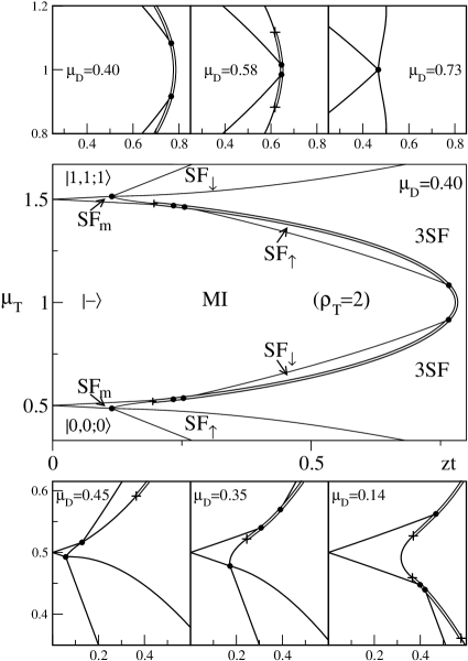
Figure 2: Center: Mean field phase diagram for $\mu_{\rm D}=0.4$, $\epsilon_{\uparrow}=\epsilon_{\downarrow}=1$, $\epsilon_{m}=2$, $g=1$, $U=V=0$, $t_{\uparrow}=t_{\downarrow}=t$, and $t_{m}=t/2$. We indicate the one-component up, down and molecular superfluids, by ${\rm SF}_{\uparrow}$, ${\rm SF}_{\downarrow}$ and ${\rm SF}_{m}$, while MI denotes the Mott insulating phase. Phase 3SF has all three components superfluid. We denote first order (continuous) transitions by double (single) lines. Junctions between phases are indicated by a dot, and the termination of first order lines by a cross. Top: Magnified portion of the central lobe tip showing the retreat of the first order transitions and the emergence of a tetracritical point. Bottom: Magnified portion of the lower left region showing the underlying tetracritical points as $\mu_{D}$ is varied.

The phase diagram has a rich structure and exhibits single component atomic and molecular condensates, and a region with all three superfluid. A notable absence is a phase where just two components are superfluid. This is a consequence of the Feshbach term (2); condensation of any two variables acts like an effective field on the remaining species and induces three component superfluidity. In contrast, condensation of a single variable no longer acts like a field and single component superfluids are supported. For example, with $\mu_{\rm D}>0$ we have $\tilde{\epsilon}_{\downarrow}>\tilde{\epsilon}_{\uparrow}$ and on leaving the vacuum we enter either the up or molecular superfluid. The former is favored at large hopping due to the chosen hopping asymmetry; see Fig. 2.

The appearance of single component atomic superfluids, with $\langle a_{\downarrow}\rangle\neq 0$ or $\langle a_{\uparrow}\rangle\neq 0$, distinguishes this from the homonuclear case Radzihovsky et al. (2004); Romans et al. (2004). In the latter, single component atomic superfluids are absent due to the reduced form of the Feshbach term $\sim g(a_{m}^{\dagger}aa+{\rm h.c.})$. This difference also shows up in the symmetry classification of the phase transitions. In the heteronuclear problem defined by equation (2), molecular condensation leaves a ${\rm U}(1)$ symmetry intact ($a_{i\downarrow}\rightarrow e^{i\alpha}a_{i\downarrow}$, $a_{i\uparrow}\rightarrow e^{-i\alpha}a_{i\uparrow}$) in contrast to the ${\mathbb{Z}}_{2}$ symmetry ($a\rightarrow-a$) of Refs. Radzihovsky et al. (2004); Romans et al. (2004). The transition from the molecular to three component superfluid is thus expected to be in the XY universality class along its continuous segment rather than Ising.

Landau Theory.— The phase diagram in Fig. 2 displays an elaborate network of quantum critical points and phase transitions. This topology reveals an underlying structure that is succinctly captured by Landau theory. In the absence of competition from other phases the locus of continuous transitions from the Mott states to the one-component superfluids may be determined analytically. This may be done using second order perturbation theory to locate the $|\phi_{\alpha}|^{2}$ terms, or through diagonalization of (3) when two $\phi_{\alpha}$ are set to zero; e.g. the transition from $|0,0;0\rangle$ to the up-superfluid with $\langle a_{i\uparrow}\rangle\equiv\phi_{\uparrow}\neq 0$ occurs along a segment of $zt_{\uparrow}=\tilde{\epsilon}_{\uparrow}$. More generally,

$$E=E_{0} +\frac{1}{2}\sum_{\alpha}m_{\alpha}|\phi_{\alpha}|^{2}+\frac{\gamma}{2}\left(\phi_{m}^{\ast}\phi_{\downarrow}\phi_{\uparrow}+{\rm h.c.}\right)$$ (4)

$$+\frac{1}{4}\sum_{\alpha\beta}\lambda_{\alpha\beta}|\phi_{\alpha}|^{2}|\phi_{\beta}|^{2}+{\mathcal{O}}(\phi^{6}),$$

where $\lambda_{\alpha\alpha}>0$, and the detailed form of the coefficients (but not the structure) depend on the unperturbed Mott state with energy $E_{0}$. This is a Bose–Hubbard ${\rm U}(1)$ Landau theory for each component Fisher et al. (1989), supplemented by couplings allowed by the ${\rm U}(1)\times{\rm U}(1)$ symmetry of (1). A similar model (without permissible biquadratic terms) was put forward on phenomenological grounds to describe pairing in the two-band Bose–Hubbard model without a Feshbach term Kuklov et al. (2004). One may gain insight into the Landau theory (4) by reduction. Near the lower tetracritical point in Fig. 2 for example, $\phi_{\downarrow}$ is massive ($m_{\downarrow}>0$) and may be eliminated using its saddle point:

$$E=E_{0}+\frac{1}{2}\sum_{\alpha}m_{\alpha}|\phi_{\alpha}|^{2}+\frac{1}{4}\sum_{\alpha\beta}\Lambda_{\alpha\beta}|\phi_{\alpha}|^{2}|\phi_{\beta}|^{2}+\dots,$$ (5)

where $\alpha,\beta=\uparrow,m$, $\Lambda_{\alpha\alpha}=\lambda_{\alpha\alpha}$ and $\Lambda_{\uparrow m}=\lambda_{\uparrow m}-\gamma^{2}/m_{\downarrow}$. The behavior of this reduced Landau theory (5) depends on the sign and magnitude of $\Lambda_{\uparrow m}$. For $\Lambda_{\uparrow\uparrow}\Lambda_{mm}>\Lambda_{\uparrow m}^{2}$ it yields a tetracritical point Chaikin and Lubensky (1995), whilst away from this, and for $\Lambda_{\uparrow m}<0$, it yields two tricritical points separated by a first order transition. This evolution is borne out in Fig. 2, where we track the development of the phase diagram as a function of $\mu_{\rm D}$. Indeed, the whole phase diagram may be understood within this reduced framework as the evolution of three such tetracritical points and their particle–hole reflections by eliminating $\phi_{\downarrow}$, $\phi_{\uparrow}$, and $\phi_{m}$ in turn.

Mott Phases.— Having surveyed the overall phase diagram we turn our attention to the Mott states. This will reveal Ising transitions in both the heteronuclear and homonuclear lattice problems, unreported in Refs. Rousseau and Denteneer (2009, 2008). To explore the central lobe where the Feshbach term is operative, we adopt a magnetic description. With a pair of atoms or a molecule at each site, we introduce effective spins $|\!\Downarrow\rangle\equiv|1,1;0\rangle$, $|\!\Uparrow\rangle\equiv|0,0;1\rangle$; see Fig. 3 (a). The operators $S^{+}=a_{m}^{\dagger}a_{\uparrow}a_{\downarrow}$, $S^{-}=a_{\downarrow}^{\dagger}a_{\uparrow}^{\dagger}a_{m}$, and $S^{z}=\left(n_{m}-n_{\downarrow}n_{\uparrow}\right)/2$, form a representation of ${\rm su}(2)$ on this reduced Hilbert space, and deep within the Mott phase we perform a strong coupling $t/U$ expansion Duan et al. (2003):

$$H=J\sum_{\langle ij\rangle}S_{i}^{z}S_{j}^{z}+\sum_{i}\left(hS_{i}^{z}+\Gamma S_{i}^{x}\right),$$ (6)

where $\Gamma=2g$ and $J=2(\frac{t_{\downarrow}^{2}+t_{\uparrow}^{2}}{U-V}+\frac{t_{m}^{2}}{2U})>0$ is antiferromagnetic exchange. We have omitted the constant, $\tilde{\epsilon}_{m}-h/2-Jz/8$ per site. This takes the form of a quantum Ising model in a longitudinal and transverse field. The longitudinal field, $h$, reflects the energetic asymmetry between a molecule $|\!\Uparrow\rangle$, and a pair of atoms $|\!\Downarrow\rangle$. The transverse field, $\Gamma\equiv 2g$, encodes Feshbach conversion; see Fig. 3 (a).

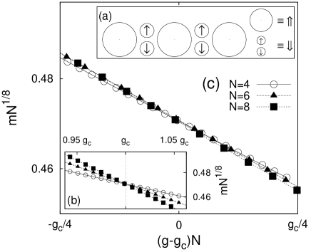
Figure 3: (a) A pair of atoms, $a_{\downarrow},a_{\uparrow}$, is represented by spin down $|\!\Downarrow\rangle$ and a molecule, $a_{m}$, by spin up $|\!\Uparrow\rangle$. Hopping favors Néel order, whilst the Feshbach term acts like a transverse field. (b) $mN^{1/8}$ versus $g$ obtained from exact diagonalization of the 1D bosonic model (1) for different system sizes, $N$ at density $\rho_{\rm T}=2$. We take $\epsilon_{\downarrow}=\epsilon_{\uparrow}=1$ and $\epsilon_{m}=2$ ($h=0$) and $U=1$, $V=0$. We set $t=t_{\uparrow}=t_{\downarrow}=2t_{m}=0.01$. The crossing point, $g_{c}\approx 1.041\times 10^{-4}$, lies slightly below the critical value, $g_{c}=J/4$, of the Ising model (6). (c) Scaling collapse as a function of $(g-g_{c})N$ with the critical exponents $\beta=1/8$ and $\nu=1$ of the 2D classical Ising model.

Since XY exchange involves interchanging two atoms and a molecule it enters at $t^{3}/U^{2}$ and may be neglected.

Numerical Simulations.— The model (6) is of considerable importance in a variety of contexts, and underpins much of our understanding of quantum magnetism and quantum phase transitions. To verify this realization in our bosonic model, we perform exact diagonalization on the 1D quantum system (1) with periodic boundaries. At present numerical techniques are considerably less advanced for multicomponent bosonic systems, and the large Hilbert space $\propto 2^{3N}$ restricts our simulations to $N=8$ sites. We begin with $h=0$ before exploring finite fields. Owing to the absence of spontaneous symmetry breaking in finite size systems, the staggered magnetization vanishes. Instead, it is convenient to focus on $m\equiv\langle|\sum_{i}(-1)^{i}S_{i}^{z}|\rangle/N$ Um et al. (2007), where $S_{i}^{z}=\left[n_{im}-(n_{i\uparrow}+n_{i\downarrow})/2\right]/2$. Adopting the finite size scaling form, $m=N^{-\beta/\nu}\bar{m}\left[(g-g_{c})N^{1/\nu}\right]$ Um et al. (2007), we plot $mN^{1/8}$ versus $g$ for different system sizes, $N$; see Fig. 3 (b). These cross close to the critical coupling, $g_{c}=J/4$, of the purely transverse field Ising model, and the scaling collapse is consistent with the critical exponents $\beta=1/8$ and $\nu=1$ for the 2D classical model. Repeating this we may track the transition within the Mott lobe. The results in Fig. 4 (b) show clear Ising behaviour at small hoppings.

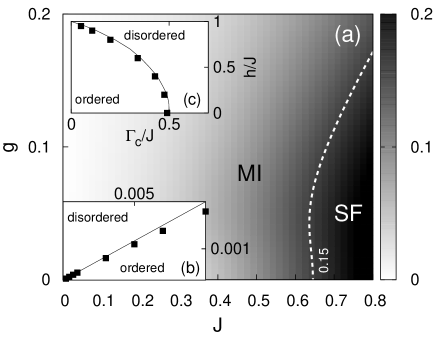
Figure 4: (a) Total SF fraction, $f_{s}$ Roth and Burnett (2003), for $N=8$ sites and the parameters used in Fig. 3. The contour indicates the approximate location of the MI-SF boundary. (b) $g$ versus $J$ showing the Ising transition $g_{c}(J)$ in the second lobe of the 1D bosonic model (1) using exact diagonalization. In the small $J$ limit, $g_{c}=J/4$ (solid line) in accordance with the transverse field Ising model. (c) $h$-dependence of $\Gamma_{c}=2g_{c}$ at fixed $J$, for the 1D bosonic (squares) and quantum Ising models (solid line). Here $\epsilon_{m}=2+h$ and all other parameters as in Fig. 3.

In addition, the finite size corrections to the ground state energy yield the central charge, $c\approx 0.51$, consistent with the exact result, $c=1/2$. At larger $J$ we continue to identify a transition in the Ising universality class, but the locus is modified. Our system sizes are insufficient to track this all the way to the superfluid boundary; see Fig. 4. These issues will be addressed in detail elsewhere by DMRG. Having established an Ising transition at $h=0$, we now consider $h\neq 0$. As shown in Fig. 4 (c), the location of the critical point evolves in accordance with exact diagonalization of (6) and DMRG results on the Ising model Ovchinnikov et al. (2003). The leading quadratic correction to the ground state energy, $\delta E_{0}^{(2)}\approx-0.07h^{2}N$ at $g=g_{c}$ Ovchinnikov et al. (2003) is also compatible . This confirms an Ising transition in our bosonic model for a range of parameters without fine tuning. This also occurs in the homonuclear problem with $\rho_{\rm T}=n_{a}+2n_{m}=2$ Rousseau and Denteneer (2009, 2008). The spins are modified due to the occupation factors (e.g. $S^{+}=m^{\dagger}aa/\sqrt{2}$) but a transition remains.

Conclusions.— We have considered the Feshbach problem for two species of bosons in an optical lattice and have obtained both a rich phase diagram and the overarching Landau theory. Within the second Mott lobe we establish a quantum phase transition described by the paradigmatic quantum Ising model. Potential experiments include magnetization distributions Lamacraft and Fendley (2008), quantum quenches Rossini et al. (2009); Calabrese and Cardy (2006), and response near quantum critical points. Realizing such models on frustrated lattices may probe connections to dimer models. Finite lifetime effects may also lead to complex coefficients, and reveal analytic properties such as the Yang–Lee edge Fisher (1978). In the light of these findings it would be interesting to revisit the numerical simulations in Refs Rousseau and Denteneer (2009, 2008). In particular, we have verified that the low excited states of the bosonic problems are described by Ising Hamiltonians deep within the Mott phase. Significantly, the lack of gapless excitations for $g>g_{c}$, and the suppression of XY exchange, suggests the absence of novel super-Mott Rousseau and Denteneer (2009, 2008) behavior in this region of the phase diagram. It would be valuable to explore this.

Acknowledgements.— We are extremely grateful to G. Conduit, F. Essler, J. Keeling, M. Köhl, D. Kovrizhin, and S. Powell for discussions. MJB, AOS, and BDS acknowledge EPSRC grant no. EP/E018130/1. MH was supported by the FWF Schrödinger grant No. J2583.

References

- Donley et al. (2002) E. A. Donley, N. R. Claussen, S. T. Thompson, and C. E. Wieman, Nature 417, 529 (2002).
- Regal et al. (2003) C. A. Regal, C. Ticknor, J. L. Bohn, and D. S. Jin, Nature 424, 47 (2003).
- Regal et al. (2004) C. A. Regal, M. Greiner, and D. S. Jin, Phys. Rev. Lett. 92, 040403 (2004).
- Radzihovsky et al. (2004) L. Radzihovsky, J. Park, and P. B. Weichman, Phys. Rev. Lett. 92, 160402 (2004).
- Romans et al. (2004) M. W. J. Romans, R. A. Duine, S. Sachdev, and H. T. C. Stoof, Phys. Rev. Lett. 93, 020405 (2004).
- Koetsier et al. (2009) A. Koetsier, P. Massignan, R. A. Duine, and H. T. C. Stoof, Phys. Rev. A 79, 063609 (2009).
- Radzihovsky et al. (2008) L. Radzihovsky, P. B. Weichman, and J. I. Park, Ann. Phys. 323, 2376 (2008).
- Rousseau and Denteneer (2009) V. G. Rousseau and P. J. H. Denteneer, Phys. Rev. Lett 102, 015301 (2009).
- Rousseau and Denteneer (2008) V. G. Rousseau and P. J. H. Denteneer, Phys. Rev. A 77, 013609 (2008).
- Santos et al. (2000) L. Santos, G. V. Shlyapnikov, P. Zoller, and M. Lewenstein, Phys. Rev. Lett. 85, 1791 (2000).
- Papp and Wieman (2006) S. B. Papp and C. E. Wieman, Phys. Rev. Lett. 97, 180404 (2006).
- Papp et al. (2008) S. B. Papp, J. M. Pino, and C. E. Wieman, Phys. Rev. Lett. 101, 040402 (2008).
- Ticknor et al. (2004) C. Ticknor, C. A. Regal, D. S. Jin, and J. L. Bohn, Phys. Rev. A 69, 042712 (2004).
- Modugno et al. (2002) G. Modugno, et al., Phys. Rev. Lett. 89, 190404 (2002).
- Catani et al. (2008) J. Catani, et al., Phys. Rev. A 77, 011603(R) (2008).
- Weber et al. (2008) C. Weber, et al., Phys. Rev. A 78, 061601(R) (2008).
- Thalhammer et al. (2008) G. Thalhammer, et al., Phys. Rev. Lett. 100, 210402 (2008).
- Thalhammer et al. (2009) G. Thalhammer, et al., New J. Phys. 11, 055044 (2009).
- Thalhammer et al. (2006) G. Thalhammer, et al., Phys. Rev. Lett. 96, 050402 (2006).
- Altman et al. (2003) E. Altman, W. Hofstetter, E. Demler, and M. D. Lukin, New J. Phys. 5, 113 (2003).
- Radzihovsky and Choi (2009) L. Radzihovsky and S. Choi, Phys. Rev. Lett. 103, 095302 (2009).
- Fisher et al. (1989) M. P. A. Fisher, P. B. Weichman, G. Grinstein, and D. S. Fisher, Phys. Rev. B 40, 546 (1989).
- Kuklov et al. (2004) A. Kuklov, N. Prokof’ev, and B. Svistunov, Phys. Rev. Lett. 92, 050402 (2004).
- Chaikin and Lubensky (1995) P. M. Chaikin and T. C. Lubensky, Principles of Condensed Matter Physics (Cambridge University Press, 1995).
- Duan et al. (2003) L. M. Duan, E. Demler, and M. D. Lukin, Phys. Rev. Lett. 91, 090402 (2003).
- Um et al. (2007) J. Um, S.-I. Lee, and B. J. Kim, J. Korean Phys. Soc. 50, 285 (2007).
- Roth and Burnett (2003) R. Roth and K. Burnett, Phys. Rev. A 68, 023604 (2003).
- Ovchinnikov et al. (2003) A. A. Ovchinnikov, D. V. Dmitriev, V. Y. Krivnov, and V. O. Cheranovskii, Phys. Rev. B 68, 214406 (2003).
- Lamacraft and Fendley (2008) A. Lamacraft and P. Fendley, Phys. Rev. Lett. 100, 165706 (2008).
- Rossini et al. (2009) D. Rossini, A. Silva, G. Mussardo, and G. E. Santoro, Phys. Rev. Lett. 102, 127204 (2009).
- Calabrese and Cardy (2006) P. Calabrese and J. Cardy, Phys. Rev. Lett. 96, 136801 (2006).
- Fisher (1978) M. E. Fisher, Phys. Rev. Lett. 40, 1610 (1978).