X-ray spectra from magnetar candidates - III. Fitting SGRs/AXPs soft X-ray emission with non-relativistic Monte Carlo models

Abstract

Within the magnetar scenario, the “twisted magnetosphere” model appears very promising in explaining the persistent X-ray emission from the Soft Gamma Repeaters and the Anomalous X-ray Pulsars (SGRs and AXPs). In the first two papers of the series, we have presented a 3D Monte Carlo code for solving radiation transport as soft, thermal photons emitted by the star surface are resonantly upscattered by the magnetospheric particles. A spectral model archive has been generated and implemented in XSPEC. Here we report on the systematic application of our spectral model to different XMM–Newton  and INTEGRAL  observations of SGRs and AXPs. We find that the synthetic spectra provide a very good fit to the data for the nearly all the source (and source states) we have analyzed.

1 Introduction

Over the last few years, increasing observational evidence has gathered in favour of the existence of “magnetars”, i.e. neutron stars (NSs) endowed with an ultra-strong magnetic field ($B\approx 10^{14}-10^{15}$ G), about ten times higher than the critical threshold at which quantum electro-dynamical (QED) effects become important ($B_{crit}\sim 4.4\times 10^{13}$ G). The family of magnetars candidates comprises two classes of sources, the anomalous X-ray pulsars (AXPs) and the soft $\gamma$-ray repeaters (SGRs). About fifteen objects are known, all characterized by similar properties: slow X-ray pulsations ($P\sim 2$–12 s), large spin-down rates ($\dot{P}\sim 10^{-13}$–$10^{-10}$ s/s), a typical persistent X-ray luminosity of $\approx 10^{34}$–10${}^{36}\ {\rm erg\,s}^{-1}$, lack of bright optical companions (favouring an interpretation in terms of isolated objects), and a high level of bursting/flaring activity which can differ among the two classes (see Woods & Thompson, 2006; Mereghetti, 2008, for recent reviews.)

Spectral data can provide key information about the physics of ultra-magnetized NSs. High-energy observations of SGRs and AXPs persistent emission cover now the $\sim 0.5$–10 (XMM–Newton /Chandra ) and $\sim 20$–200 (INTEGRAL ) keV bands. It is possible, although not proved yet, that different emission mechanisms are responsible for the emission in the two bands.

The low-energy ($\la 10$ keV) spectrum of the persistent (i.e. outside bursts) emission is often modelled in terms of a blackbody ($kT\sim 0.3$–0.6 keV) plus a power-law with photon index $\Gamma_{s}\sim 2$–4, although in some AXPs a two blackbody model has been also applied. The X-ray persistent emission above 20 keV has a power-law spectral shape ($\Gamma_{h}\sim 2$) which, in particular in AXPs, is markedly harder than that observed below 10 keV (see again Mereghetti, 2008, and references therein). However, although these phenomenological fitting models have been systematically applied over the last decade, a convincing physical interpretation of the various spectral components is still missing.

In the magnetar framework, the twisted magnetosphere model (Duncan & Thompson, 1992; Thompson & Duncan, 1993; Thompson, Lyutikov & Kulkarni, 2002) offers a promising physical interpretation for the X-ray emission from SGRs/AXPs. In particular, the supporting currents required to sustain the twist are substantially in excess of the Goldreich-Julian current and can produce large optical depth to resonant cyclotron scattering (RCS). Soft (thermal) photons produced at the star surface gain energy in repeated scatterings and this leads to the formation of an extended, high-energy tail, superimposed to the seed thermal component. The qualitative predictions of this model have been verified to match some spectral and timing properties of magnetar sources, as the spectral shape observed in quiescence below $\sim 10$ keV and the long term variation observed in some sources (e.g. Mereghetti et al., 2005b; Rea et al., 2005; Campana et al., 2007).

More recently, several efforts have been carried out recently in order to test the model quantitatively against real data using different approaches and with a varying degree of sophistication. A first attempt in this direction has been presented by Lyutikov & Gavriil (2006). These authors developed a very simple, semi-analytical treatment of the RCS process by working in 1-dimensional geometry. They assumed that seed photons are emitted by the NS surface with a blackbody spectrum, and Thomson scattering occurs in a thin, plane parallel magnetospheric slab permeated by a static, non-relativistic, warm medium at constant electron density. These models have been implemented in XSPEC by Rea et al. (2007a, b, 2008) and successfully applied to all magnetars spectra below 10keV. The good agreement found, even within a simplified treatment, supports the idea that RCS in a sheared magnetosphere plays a central role is the formation of magnetar spectra in the (soft) X-ray range. The same RCS model has been used by Güver, et al. (2007), who assumed that seed photons comes from an atmosphere surrounding the star. More recently, 3-D Monte Carlo calculations have been presented by Fernandez & Thompson (2007), although these spectra have never been applied to fit X-ray observations.

Motivated by this, we present here a systematic application of our 3D Monte Carlo spectral calculations (see Nobili, Turolla & Zane, 2008a, b, for all details) to AXPs and SGRs spectral data. The paper is organized as follows. In § 2 we briefly summarize the basic features of the model. The data sample and spectral results are presented in § 3. Discussion and conclusions follow in §§ 4, 5.

2 The model

As discussed in detail in Nobili, Turolla & Zane (2008a, b), we have recently developed a 3-dimensional treatment of RCS, aimed at a detailed investigation of the spectral, timing and polarization properties of magnetars (see also Pavan et al., 2009). Our Monte Carlo code, which is completely general and can handle different magnetic field topologies and distributions of seed photons, has been used to produce an archive of spectral models that have been subsequently implemented in XSPEC. Such models rely on a number of choices for the assumed configuration, that are discussed in detail in Nobili, Turolla & Zane (2008a) and briefly summarized in this section.

First, the XSPEC archive models have been computed by assuming that the star surface emits as a blackbody at an uniform temperature, $kT$, and that the surface radiation is isotropic and unpolarized. The magnetic field topology is assumed to be a twisted, force free dipole and is uniquely characterized by the value of the twist angle, $\Delta\phi$ (see Thompson, Lyutikov & Kulkarni, 2002). No attempt is made to fit the value of the polar field strength, that has been fixed at $10^{14}$ G. Our model is based on a simplified treatment of the charge carriers velocity distribution which accounts for the particle collective motion, in addition to the thermal one. Pair production has been neglected. Magnetospheric electrons stream freely along the field lines (the motion across the field lines is quantized). The electron velocity distribution parallel to the field is taken to be a 1-D relativistic Maxwellian at temperature $T_{e}$, superimposed to a bulk motion with velocity $\beta_{bulk}$ (in units of the light velocity $c$). Besides, in order to minimize the number of free parameters, the models in the archive were computed assuming that the electron temperature is related to $\beta_{bulk}$ (see Nobili, Turolla & Zane, 2008a, for all details). Scattering in a magnetized medium was treated by considering only the resonant part of the magnetic Thomson cross section and neglecting electron recoil along the field direction. For the sake of conciseness, in the following this approximation will be referred to as the (resonant) Thomson limit. On the other hand, the code is completely general and inclusion of the relativistic QED resonant cross section, which is required in the modelling of the hard ($\sim 20$–200 keV) spectral tails observed in the magnetar candidates, is under way (see Nobili, Turolla & Zane, 2008b; Pavan et al., 2009). Electron recoil in the direction parallel to the field starts to be important when the photon energy in the electron rest frame becomes comparable to the electron rest energy. If $\gamma$ is the mean electron Lorentz factor, this occurs at typical energies $\sim m_{e}c^{2}/\gamma$. Assuming mildly relativistic particles, the previous limit implies that conservative scattering should provide good accuracy up to photon energies of some tens of keV. This, together with the fact that resonant scattering occurs in regions where $B\ll B_{crit}$, makes the use of the (much simpler) non-relativistic (Thomson) magnetic cross section adequate. The final XSPEC atable spectral model (22 MB in size, named ntznoang.mod, hereafter NTZ) has been created by using the routine wftbmd, available on-line. In summary, it depends on four free parameters ($\beta_{bulk}$, $\Delta\phi$, $\log kT$ plus a normalization constant), which can be simultaneously varied during the spectral fitting following the standard $\chi^{2}$ minimization technique. In NTZ models the photon number is conserved and the monochromatic number flux which reaches infinity is the same as that of the seed blackbody spectrum. This implies that the normalization constant (norm) divided by $kT^{3}$ is proportional to the emitting area on the star surface (see §4.2). It is important to note that the NTZ model has the same number of free parameters than the canonical blackbody plus power-law empirical model or the 1D RCS model recently discussed in Rea et al. (2008), and hence has the same statistical significance. In the following sections we present its systematic application to the soft (0.5–10 keV) X-ray spectra of magnetar candidates.

3 Application to magnetar’s soft X-ray spectra

We applied the NTZ model to a large sample of AXPs and SGRs, using XMM–Newton   and INTEGRAL   data. The sample of datasets basically coincides with that used in Rea et al. (2008), and we refer to that paper for more details and for a discussion on the data analysis. However, at variance with Rea et al. (2008), we did not consider here the transient magnetars XTE J1810-197   and CXOU J1647-4552 , the analysis of which will be reported in a separate paper devoted to a detailed investigation of their outburst evolution over a period of several years. On the other hand, we included the recent XMM–Newton   observations of CXOU J0100-7211   and SGR 1627-41 , that were not available at the time of the previous investigation (see Tiengo et al., 2008; Esposito et al., 2008, for further details on these observations).

All fits have been performed using XSPEC version 11.3 and 12.0, for a consistency check. A 2% systematic error was added to the data to partially account for uncertainties in instrumental calibrations. Only in the case of CXOU J0100-7211 , which has a very low absorbtion, the fit has been performed in the 0.5–10 keV energy range. For the other sources, that are highly absorbed, the 0.5–1 keV energy range (0.5–2 keV energy range in the case of SGR 1627-41 ) was excluded from our spectral fitting. We then checked that, for all our targets, the values of $N_{H}$ derived fitting the 1–10 keV EPIC-pn spectra, are consistent (within $1\,\sigma$) with those obtained using the 0.5–10 keV range relative to the same data set. We used the more updated solar abundances by Lodders (2003), instead of the older ones from Anders & Grevesse (1989). As a consequence, the value of the absorption is, on average, slightly higher than that reported in the literature for the same model. This does not affect the other spectral parameters.

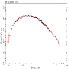
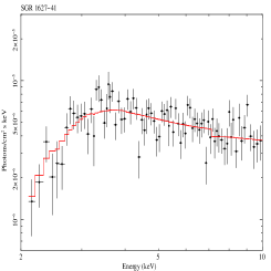
Figure 2: Same as in Fig. 1 for CXOU J0100-7211   and SGR 1627-41 . See Table 1 for details.

Table 1 and Figs. 1, 2 report our results in the 1–10 keV range for those sources that do not show a substantial spectral variation, in which cases only one dataset (the longest available) has been considered. Also, in Tables 2, 3 and Fig. 3 we show the fits for sources that do exhibit spectral variation, in which cases we considered a set of two–three observations for each source, corresponding to different spectral states. At variance with Rea et al. (2008), in these cases the different datasets have been fitted by imposing that the absorption, $N_{H}$, is the same. As it can be seen from the tables, in most of the cases we found that a NTZ model alone successfully reproduces the soft X-ray part of the spectrum up to 10 keV, without the need of further components (see §4 for a discussion). With reference to the sample considered in Rea et al. (2008), the only two sources for which we do not find a satisfactory fit are 1E 2259+586  and 4U 0142+614 , which are discussed separately below.

There are a few AXPs and SGRs in our sample (namely 1RXS J1708-4009 , 1E 1841-045 , 4U 0142+614 , 1E 2259+586 , SGR 1900+14 and SGR 1806-20 ) that are known to have a conspicuous emission in the hard X-ray band. For these objects we have repeated our modelling including also their INTEGRAL   spectra in order to investigate whether our model can reproduce part of the emission when considering the whole SED. A further power-law (PL) has been introduced in order to account for the non thermal hard X-ray component, although at a purely phenomenological level. A free constant was multiplied when using both XMM–Newton   and INTEGRAL   data to account for inter-calibration uncertainties (the values of the constant was always differing by less than 10% with respect to XMM–Newton   which was set to unity). Results are reported in Table 4 and Fig. 4. We find that, again with the exception of 1E 2259+586  and 4U 0142+614 , in all other cases a NTZ+PL spectral decomposition successfully models the 1–200 keV emission. However, the fit converges with a hard X-ray component that gives a substantial contribution when extrapolated to the soft X-ray band and, consequently, the best fitting parameters of the NTZ model are substantially different from those we found fitting the 1-10 keV emission only.

As the tables show, in some cases the fit converges with a value of $\Delta\phi$ which is too close to the upper bound of our model archive ($\Delta\phi=2$), making impossible to compute the whole (closed) $1\sigma$ contour level. Indeed, in the case of the combined XMM–Newton  and INTEGRAL  fits of 1E 1841-045  and SGR 1900+14 , the parameters of the NTZ model becomes less constrained than when fitting the XMM–Newton  data alone, and we could only set an upper limit on $\Delta\phi$ (see Table 4). Although we do not regard this as a particular problem, we should caveat that in some fits the value of the twist angle appears to be less constrained than those of the other model parameters.

4 Discussion

In this paper we have applied a 3D Monte Carlo model of resonant scattering to the phase averaged spectra of an extensive set of magnetar sources. The sample is the same as in Rea et al. (2008), with the exception of the two transient magnetars XTE J1810-197   and CXOU J1647-4552 , and with the inclusion of recent XMM–Newton   observations of CXOU J0100-7211   and SGR 1627-41 . The discussion of our findings is organized as follows. In §4.1, we first concentrate on the results emerging from the fit of the XMM–Newton  data only, i.e. on the energy band below 10 keV. We report the discussion of our spectral results, a comparison with the analogous findings from the 1D RCS fits of Rea et al. (2008), and we discuss the cases of 1E 2259+586  and 4U 0142+614 , i.e. the only two sources for which a fit with the NTZ model is unsatisfactory. A search for correlations among the sources and the model parameters, in the same energy band, is reported in $4.2. In $4.3 we then discuss the NTZ model in the contest of the interpretation of the whole SED up to $\sim$200 keV, basing this time on both XMM–Newton  and INTEGRAL  data. The main limitations and caveats are then summariszed in $4.4.

4.1 The soft X-ray spectra: fits of the XMM–Newton  data

Our results on the fits of the XMM–Newton  data are reported in Tab. 1, and Figs. 1,2 for sources without a significant spectral variation, and in Tables 2, 3 and Fig. 3 for sources that do exhibit spectral variation. When we restrict to the 1–10 keV band, we found that the NTZ model successfully reproduces the soft X-ray part of the spectrum of most of the sources (apart from 1E 2259+586  and 4U 0142+614 ), without the need of additional components. This represents a substantial improvement with respect to previous attempts to model magnetars quiescent emission in the same energy band with a simpler 1D RCS model (Rea et al., 2008), where it was found that in a few cases a PL component was required, in addition to the RCS one, to provide an acceptable fit to the data below 10 keV. In particular, this was the case of few AXPs (including e.g. 1RXS J1708-4009 and 1E 1841-045 ) and of SGR 1806-20 , all them detected also above $\ga 20$ keV. In such cases, we found that the 1D RCS component reproduces the spectrum only up to 5–8 keV. In order to match the data at the highest XMM–Newton  energies, the contribution of a PL must be included. On the other hand, the slope of this additional PL is the same of that describing the INTEGRAL  spectrum in the $\sim 20$–200 keV band. It is well possible that the mechanism responsible for the hard X-ray emission provides a non negligible contribution in the soft X-ray range. However, our finding is that the resonant Compton scattering model by Nobili, Turolla & Zane (2008a) correctly describes the data in the whole XMM–Newton  energy range, i.e. up to 10 keV, for all the sources (and source states) reported in Tables 1,2,3. The application of the NTZ model to the $\ga 20$ keV emission from magnetars is discussed later on. It is worth noticing that the NTZ model has two free parameters less than the 1D RCS+PL model used in Rea et al. (2008). Hence, besides self-consistency, it is also more robust on a statistical ground.

In all cases we found that $N_{H}$, as derived from the NTZ model, is lower than (or consistent with) that inferred from the BB+PL fit, and consistent with what derived from fitting the single X-ray edges (Durant & van Kerkwijk 2006). The same was also true for the fits with the 1D RCS model presented in Rea et al. (2008). This is not surprising, since the power-law usually fitted to magnetar spectra in the soft X-ray range is well known to overestimate the column density. The surface temperature we derived fitting the NTZ model is slightly higher than the corresponding 1D RCS temperature and consistent with the BB temperature in the BB+PL model. On the other hand, a quantitative comparison between the values of $\beta_{bulk}$ and $\Delta\phi$, i.e. the parameters that describe the magnetospheric currents in the NTZ model, with the corresponding parameters of the 1D RCS model ($\beta_{T}$ and $\tau_{res}$) is more difficult, due to the different assumptions about the currents velocity distribution and the magnetic field topology. The 1D RCS assumes a plane parallel slab (i.e. photons can only propagate along the slab normal, either towards or away from the star). Moreover, magnetospheric charges are assumed to have a top-hat velocity distribution centered at zero and extending up to a given temperature, $\pm kT_{e}$. To some extent, this scenario mimics a thermal, 1D, motion (in which case $kT_{e}$ can be assimilated to a mean $e^{-}$ energy, i.e. to the temperature of the 1D electron plasma). Since the $e^{-}$ velocity distribution averages to zero, no bulk motion is accounted for: if we only consider the frequency shift due to the $e^{-}$ motion then a photon has the same probability to undergo up or down scattering. Photon boosting by particle thermal motion in Thomson limit may still occur, because the spatial variation of the magnetic field is taken into account. For a photon propagating from high to low magnetic fields, multiple resonant cyclotron scattering will, on average, up-scatter the transmitted radiation, giving rise to the formation of an hard tail. Since, at variance with the 1D RCS model, our code accounts for both bulk and thermal motion, one may expect to find a value of $\beta_{bulk}$ systematically lower than the value of the velocity parameter $\beta_{T}$ in the 1D RCS fits. However, we find that this is not always the case and the relation between the values of $\beta_{bulk}$ and $\beta_{T}$ appears to be more complex. The NTZ model does not explicitly contain the optical depth as a parameter. However, $\Delta\phi$ and $\beta_{bulk}$ can be related to the (average) scattering depth, as discussed in Rea et al. (2008). In particular, the value of $\tau_{ave}$ can be read off from their figure 10, simply by dividing the value of the depth corresponding to a given $\Delta\phi$ by $\beta_{bulk}$. The values of $\tau_{ave}$ we derive ($\sim 0.1$–1, as expected since the average number of scatterings for a typical photon is of this order) are systematically lower than those obtained for the 1D RCS $\tau_{res}$. This means that the 1D RCS model is intrinsically less efficient in up-scattering the seed photons. Its spectrum is, in fact, softer and it requires a larger depth (and hence a larger number of scatterings). Moreover, the hardest sources require an additional PL to match the observed XMM–Newton  spectra. When observations of the same source at different epochs are available, it is of interest to check if the best-fit values of the model parameters change, since this can reveal how the physical properties of the surface/magnetosphere evolve in time. In the case of 1E 1048-5937  all the parameters are compatible with being constant within the errors, with the only exception of the normalization which appears to increase following the flux rise. The same holds for SGR 1806-20   where there may be also an indication for a decrease in the twist angle after the giant flare of December 27th 2004. Errors are however quite large and prevent any firm conclusion at this stage. The time behaviour of 1E 1547.0-5408  is puzzling, since $\beta_{bulk}$ increases while $\Delta\phi$ decreases as the flux, and the model normalization, increases. In this source there is also a quite robust evidence that the surface temperature increased with the flux.

As we mentioned before, in the case of 1E 2259+586  and 4U 0142+614  we were unable to find a satisfactory fit with the NTZ model. We noticed that, below 10 keV, these two sources are characterized by a rather soft spectrum: in the canonical BB+PL decomposition the power law index is $\sim 4$ instead of $\sim 2-3$ as in other magnetars. At the same time, the power law tail starts very close to the energy at which the BB peaks. Such a spectral shape appears difficult to explain in terms of upscattering of soft photon, whatever the nature of the comptonization process might be. In fact, a PL component that starts close to the BB peak is a signature of a full fledged comptonization in which case, however, it is expected to be quite flat. Conversely, a steep power law tail is typical of weak comptonization and departures from the BB spectrum occur at energies beyond the peak. One possible explanation is that the BB peak appears to be less prominent to the observer because the region that emits the soft seed photons is not coming completely into view. In Nobili, Turolla & Zane (2008a), we considered the effects of a non-homogeneous surface temperature distribution, by examining the case in which photons are emitted by a single surface patch. In Fig. 5 we show the results of our simulations in the case in which the emitting region is confined to an equatorial strip (left panel) or to a polar cap (right panel). The subdivision of the star surface, that of the sky, the energy range and bin width are the same as that used in Nobili, Turolla & Zane (2008a; see Fig 7 in that paper). The different curves show the emerging spectrum, as viewed by an observer whose line of sight (LOS) makes an angle $\Theta_{s}$ with the spin axis and for different values of the observing longitude, $\Phi_{s}=20^{\circ},\,140^{\circ},\,220^{\circ}$. These three values correspond to having the emitting surface patch in full view (seen nearly face on), partially in view and almost screened by the star. As it can be seen, when the emitting patch is in full view the observed spectrum consists of a well visible thermal component and an extended power-law-like tail. On the other hand, if the emitting region is not directly visible, no contribution from the primary blackbody photons is present: the spectrum, which is made up only by those photons which after scattering propagate “backwards”, has a depressed thermal peak and a much more distinct non-thermal shape. In particular, in the examples of Fig. 5, the scattering efficiency is not very high and curves corresponding to $\Phi_{s}=220^{\circ}$ have a steep power-law tail with photon index $\sim 4$, as observed in 1E 2259+586  and 4U 0142+614 . Although a quantitative fit of the spectra of these two sources including different thermal maps in the code would be unfeasible (because it would introduce too many degrees of freedom), it is tempting to speculate that the peculiar spectrum of 1E 2259+586  and 4U 0142+614   is due to a strong inhomogeneity in the surface temperature distribution, with the hotter region almost antipodal with respect to the observer. This is also compatible with the fact that these two sources have a rather low pulsed fraction with respect to other magnetars. On the other hand, the double peaked pulse profile of 1E 2259+586  is difficult to explain in this picture. Another possibility is that the phase average spectrum appears to be quite soft because it reflects the contribution of different components. As discussed by Woods et al. (2004) and Rea et al. (2007c), both these sources exhibit a strong spectral variation with spin phase. In the case of 4U 0142+614  the spectrum switches from being very hard to very soft within a 0.1-wide phase interval and XMM–Newton   data reveals a discontinuity, between 2 keV and 3 keV, which can be interpreted as a curved component and is most appearent within phase interval 0.7-0.9 (Den Hartog et al., 2008a). In order to assess this scenario, a more detailed investigation of the pulse resolved spectra is necessary; this requires the introduction of the viewing geometry in our fits and will be presented in a forthcoming paper.

4.2 Correlations

We run a number of Spearman’s rank correlation tests, in order to look for possible links among the observed properties of the sources in our sample and the model parameters. In particular, we checked for correlations between the 1–10 keV luminosity, $L_{1-10\,{\rm keV}}$ or the spin-down value of the magnetic field, $B$, and each of the NTZ parameters, $kT$, $\beta_{bulk}$, and $\Delta\phi$. The values of the parameters are those obtained from the fit of the XMM–Newton  data only (Tables 1,  2,  3). The source distances and the values of $B$ have been taken from the compilation in Rea et al. (2008). The only significant correlations which emerged are those between $\beta_{bulk}$ and $L_{1-10\,{\rm keV}}$ and $\beta_{bulk}$ and $B$. Both show a deviation from the null hypothesis probability of $\sim 93\%$. Although the significance level is lower, $81\%$, a correlation between $kT$ and $L_{1-10\,{\rm keV}}$ seems also to be present. The correlation between $L_{1-10\,{\rm keV}}$ and $\beta_{bulk}$, which is direct, can be explained taking into account that an increase of $\beta_{bulk}$ results in a larger energy gain of the photons per scattering and hence in a hardening of the spectrum, which translates into a higher luminosity. A similar argument applies to the $L_{1-10\,{\rm keV}}$–$kT$ correlation, which is again direct. An increase of the surface temperature implies an increase of the flux of primary photons and again of the observed luminosity. The $\beta_{bulk}$–$B$ correlation mirrors that between $\beta_{T}$ and $B$ reported in Rea et al. (2008), and, as discussed there, is not of immediate interpretation.

As discussed in Nobili, Turolla & Zane (2008a), the modulation of the X-ray flux may be due to the anisotropy of the magnetospheric charge density (which is lower along the poles), to a patchy surface temperature distribution, or to a combination of both effects. As mentioned in §2, in NTZ models the normalization constant (norm) divided by $kT^{3}$ is proportional to the emitting area on the star surface. To check if the observed modulation is related (also) to the presence of a hotter region on the surface, we looked for a correlation between the pulsed fraction and the ratio norm$\times D^{2}/kT^{3}$, where $D$ is the source distance. The pulsed fraction is defined as the semiamplitude of the sinusoidal function that best-fits the lightcurve, in the same energy range. We run the test on the entire sample of sources, excluding the first observation of 1E 1547.0-5408 , for which only an upper limit of the pulsed fraction is available. No significant correlation was found. However, when the sample is restricted to AXPs only, a negative correlation (i.e. the pulsed fraction increases when the area decreases) emerges at the $91\%$ confidence level. To verify this, we run again the test including the data from a set of five more recent observations of 1E 1547.0-5408  (Bernardini et al., in preparation) and found that the correlation is still present, although the significance level slightly decreases to $74\%$ (see Fig. 6). Taken face value, this results points towards a localized emitting area in AXPs while the surface temperature would be more uniform in SGRs, where the modulation is produced mainly by scatterings in the magnetosphere. We note that the presence of a (time varying) hot spot has been reported in some transient AXPs, but the existence of a general pattern as the one discussed above needs a larger sample to be confirmed.

Finally, we checked if there is a correlation between $\Delta\phi$ and $\beta_{bulk}$. The motivation for this is that both parameters are responsible for the formation of the high-energy tail. This may introduce a redundancy in the model parameters: in principle the fit might be not unique, since quite similar spectra may be obtained with different combinations of $\Delta\phi$ and $\beta_{bulk}$ (e.g. low $\beta_{bulk}$ and large $\Delta\phi$ or the opposite). We did not find any significant correlation between these two quantities.

4.3 The broadband spectrum in the 1-100 keV range.

As discussed in §3, a spectral decomposition of the kind NTZ+PL successfully reproduces the whole spectrum of 1RXS J1708-4009 , 1E 1841-045 , and SGR 1900+14 , up to 200 keV. In this case, however, the best fit parameters of the NTZ model differ from those found from the fit of XMM–Newton  data up to 10 keV. In particular, while the temperature of the seed blackbody is almost unchanged, the value of $\beta_{bulk}$ is always considerably reduced (from 0.3-0.5 down to 0.1-0.2) and the twist angle less constrained. This indicates that in the broadband fit most of the hardening is accounted for by the additional PL component that, in the case of 1E 1841-045  and SGR 1900+14 , starts to dominate the spectrum at energies as low as $\sim$3–4 keV. Of course, this kind of spectral decomposition is certainly possible and may mimic a scenario in which the hard X-ray and soft X-ray emissions are due to two separate processes: for instance soft $\gamma$-rays may be produced in a twisted magnetosphere by thermal bremsstrahlung emission from the surface region heated by returning currents, or synchrotron emission from pairs created higher up ($\sim$ 100 km) in the magnetosphere (Thompson & Belobodorov, 2005).

In principle, however, spectra produced by resonant cyclotron upscattering of soft photons are expected to develop power law tails that extend up to much higher energies (Baring & Harding, 2007; Nobili, Turolla & Zane, 2008a). Therefore, it is well possible that our model can consistently explain the whole spectral energy distribution in the 1-200 keV range. If this is the case, the slope of the hard power law tail would be mainly dictated by the properties of the magnetospheric electrons responsible for the upscattering, i.e. their density and velocity distribution. Observationally the hard X-ray properties of AXPs and SGRs are quite different: while in the range 4-200 keV the spectra of SGRs are dominated by the non-terhmal component and, in the canonical model, well reproduced by a single unbroken PL, AXPs show a sort of turn over and have a non-thermal tail which is initially softer, up to $\sim 5-8$ keV, and then flattens at higher energies. In this picture, 1E 1841-045   seems an exception: its non-thermal emission is well reproduced by a single PL and is therefore more SGR-like (see Rea et al., 2008, and references therein). These properties suggest that, within the resonant Compton scattering scenario, AXPs spectra require different electron populations. On the other hand, a single electron distribution as for instance the one we used in the 3D computations presented here, may account for the broadband emission of SGRs or SGR-like sources.

In order to test this possibility, we can not use directly our XSPEC table of models, since it has been computed assuming that magnetic scattering is conservative in the electron frame and, for self-consistency, spectra were truncated at 15 keV (see § 2 for a discussion). Instead, we re-computed the model that best-fits the 1-10 keV spectrum of SGR 1900+14 (which parameters are reported in Table 1), this time by extending the computation to the whole 1-200 keV energy range and using a fully relativistic version of the Monte Carlo code which incorporates the complete QED scattering cross section (Nobili, Turolla & Zane, 2008b). We also repeated the computation by using slightly different sets of parameters, all within $3\sigma$ from their best-fitting values (errors at $1\sigma$ are reported in Table 1). As expected, these new spectra differ from those computed in the Thomson limit only at very high energies ($>100$ keV). Finally, we added to each curve a free normalization constant in the INTEGRAL  range, to account for inter-calibration uncertainties between the two satellites. We then fitted the INTEGRAL  data by leaving only the intercalibration constant as a free parameter. Results are reported in Fig. 7, where the two curves correspond to: i) the best fitting parameters reported in Table 1 and ii) to a different model in which $\beta_{bulk}$, $kT$ and $\Delta\phi$ have been increased up to their upper limits within the $3\sigma$ confidence range from the XMM–Newton  fit. We found that in both cases the fit to INTEGRAL  data is excellent (reduced $\chi^{2}=1.14$ and 1.07, respectively, for 7 degrees of freedom), but the two model normalizations, in the XMM–Newton  and INTEGRAL  ranges, differ by a factor 8.8 and 2.8 respectively, too large to be attributed to intercalibrations uncertainties. Not surprisingly, similar large factors are also found when trying to fit the XMM–Newton  and INTEGRAL  data in the range 6-200 keV with a simple power law model. On the other hand, this simple test proves that the spectral slope of our model in the 20-200 keV range is the same as that of the INTEGRAL  data. Similar considerations hold in the case of 1E 1841-045 . Although a conclusive answer requires a direct fitting of the combined XMM–Newton  and INTEGRAL  data with a self-consistent Compton model, which is beyond the scope of this paper, we regard this preliminary finding as promising.

4.4 Caveats and future developments

We caveat that the models presented here are based on a number of simplifying assumptions. First, they are based on a globally twisted dipole model, that only gives an idealized representation of the magnetic field topology. There are now both theoretical (Beloborodov, 2009) and observational (a certain degree of hysteresis in the long-term evolution of SGR 1806-20, Woods et al. 2007; the long-term evolution of the thermal component of the transient AXP XTE J1810-197, Perna & Gotthelf 2008; Bernardini et al. 2008) motivations in favour of a picture in which the twist affects only a limited portion the magnetosphere, typically the polar region. Furthermore, phase resolved spectroscopy of the two AXPs 1RXS J1708-4009 and 4U 0142+61 in the INTEGRAL  energy range (Den Hartog et al., 2008a, b) shows dramatic spectral changes with the spin phase. It has been recently suggested that a resonant scattering model in which the magnetic field is locally twisted may catch the essential features of this behaviour (Pavan et al., 2009).

A further point is the nature and velocity distribution of the magnetospheric charges. The NTZ model assumes the presence of mildly relativistic electrons, moving at constant velocity (which is a model parameter) along the closed field lines. Currents flowing in the magnetosphere of a magnetar have been investigated by Beloborodov & Thompson (2007), who concluded that the magnetosphere is populated by pairs with a Lorentz factor $\gamma\approx 1000$. However, more recent calculations (Nobili, Turolla & Zane, in preparation) show that in the region where $B\ga 2B_{Q}$ Compton losses efficiently slow down electrons, limiting pair creation to a small region close to the star surface, and allowing for the presence of mildly relativistic particles along much of the circuit.

Finally, angle of view effects have not been accounted for: the emerging spectrum is simply computed by integrating over the whole sky at infinity. This corresponds to the case in which the star is an aligned rotator, i.e the spin and magnetic axes coincide. As discussed in Nobili, Turolla & Zane (2008a), in order to treat the more general case in which the spin and magnetic axes are not aligned, we also produced a second XSPEC atable model by introducing two angles, $\chi$ and $\xi$, which give, respectively, the inclination of the LOS and of the dipole axis with respect to the star spin axis. This allows us to take into account for the star rotation and hence derive pulse shapes and phase-resolved spectroscopy. The spectral model, ntzang.mod, has six free parameters ($\beta_{bulk}$, $\Delta\phi$, $\log kT$, $\chi$, $\xi$ plus a normalization constant), i.e. two more than the one used here. Given that the NTZ model produces a very good fit for the phase-averaged spectra, the inclusion of two further parameters (i.e. the two angles) is not statistically required, as we tested, and will leave $\chi$ and $\xi$ unconstrained. On the other hand, having the possibility to infer the viewing geometry may be useful when fitting different outburst states in transient AXPs or when combining information that can be obtained by fitting simultaneously phase-resolved spectra, or independently from the study of the pulse profile. Further work in this direction is under way and will be presented in separate papers.

5 Conclusions

By considering a large sample of magnetars, we found that resonant Compton upscattering by a population of mildly relativistic electrons ($\beta_{bulk}\sim 0.1--0.7$) can reproduce the pulse averaged spectra in the range 1–10 keV. At variance with the 1D RCS model adopted in Rea et al. (2008), the approach used in the present investigation consistently accounts for the bulk motion of magnetospheric electrons which results in a more efficient comptonization of seed thermal photons. This has two main consequences: i) the required values of the optical depth are lower that those found using the 1D RCS, and ii) NTZ spectra, being intrinsically harder, successfully reproduce also the SGRs power-law tail below 10 keV. We found a significant correlation between the 1–10 keV source luminosity and both $\beta_{bulk}$ and $kT$. This is indeed expected in the resonant cyclotron scattering model and further supports this scenario to explain the high energy emission from magnetars. Moreover, when restricting to AXPs only, we find hints for a negative correlation between the pulsed fraction and the emitting area. If confirmed, this suggests the presence of a strong thermal gradient on the star surface, which may also be responsible for the slightly different spectrum of 4U 0142+614  and 1E 2259+586 , the only two sources for which we could not find a satisfactory fit. Anisotropic surface thermal distributions may arise in the presence of large crustal magnetic fields, as expected in magnetars, because heat is preferentially transferred along the field, resulting in small and confined hot caps (e.g. Geppert, Kueker & Page, 2006; Pons, Miralles & Geppert, 2009). Moreover, the magnetar surface is also expected to be further heated during bursting activity or by returning currents; in both cases the heat deposition can be substantially anisotropic.

Finally, our conclusions regarding the modelling of the whole SED distribution up to $\sim 200$ keV are still compatible with various scenarios. In the case of 1E 1841-045 , 1RXS J1708-4009 , and SGR 1900+14 , a double component NTZ+PL model fits the combined XMM–Newton  and INTEGRAL  data, but it requires a NTZ spectrum quite soft and most of the emission dominated by the additional PL. This is compatible with a scenario in which soft X-ray and hard X-ray emission are ascribed to independent components. On the other hand, there is also the possibility that models of resonant upscattering can successfully describe the whole SED including the hard X-ray tail (eventually by invoking more than one electron population for sources with a spectral turnover at high energies). A conclusive answer requires a direct fitting of the combined XMM–Newton  and INTEGRAL  data, with all parameters left free and a new XSPEC table of models computed by using the QED cross sections. Further work on these topics is in preparation.

	1RXS J1708–4009∗	1E 1841–045	SGR 1900+14	CXOU J0100-7211	SGR 1627-41
Parameters
NH	1.45$\pm$0.08	2.5$\pm$0.1	3.74$\pm$0.15	$<0.05$	12$\pm$1
kT (keV)	0.47$\pm 0.09$	0.50$\pm 0.06$	0.45$\pm$0.04	0.35 $\pm$0.02	0.64$\pm 0.11$
$\beta_{bulk}$	0.34$\pm$0.04	0.43$\pm$0.05	0.46$\pm$0.05	0.18$\pm$0.03	0.7$\pm$0.1
$\Delta\phi$	0.49$\pm$0.15	0.47$\pm$0.04	0.45$\pm$0.03	1.7$\pm$0.8	1.3$\pm$0.4
NTZ norm	0.35$\pm$0.04	0.20$\pm$0.02	0.08$\pm$0.02	0.004$\pm$0.001	0.005$\pm$0.001
Flux (1–10 keV)	$(2.6\pm 0.2)\times 10^{-11}$	$(2.1\pm 0.2)\times 10^{-11}$	$(3.9\pm 0.3)\times 10^{-12}$	$(3.3\pm 0.2)\times 10^{-13}$	$(3.3\pm 0.2)\times 10^{-13}$
$\chi^{2}_{\nu}$ (dof)	0.97 (197)	1.04 (152)	0.99 (135)	1.21 (101)	1.16 (81)

Table 1: Spectral Parameters of 1RXS J1708-4009 , 1E 1841-045 , SGR 1900+14 , CXOU J0100-7211 , and SGR 1627-41  obtained by fitting the XMM–Newton  data with an NTZ model. The fit has been restricted to the 1–10 keV range, with the exception of CXOU J0100-7211  and SGR 1627-41  for which we used the 0.1–10 keV and 2–10 keV band, respectively. Errors are at 1$\sigma$ confidence level, reported fluxes are absorbed and in units of erg s^-1cm^-2. N_H is in units of $10^{22}$ cm^-2 and we assumed solar abundances from Lodders (2003). See also Fig. 1, 2 and § 3 for details.
^∗: source slightly variable in flux and spectrum, see text for details.

	1E 1547.0-5408		1E 1048-5937
Parameters	2006	2007	2003	2005	2007
NH	4.6$\pm$0.13		0.66$\pm$0.02
kT (keV)	0.38$\pm$0.01	0.56$\pm$0.01	0.60$\pm 0.06$	0.56$\pm 0.08$	0.69$\pm$0.02
$\beta_{bulk}$	0.15$\pm$0.05	0.4$\pm$0.1	0.14$\pm$0.03	0.16$\pm$0.07	0.13$\pm$0.04
$\Delta\phi$	1.14$\pm$0.08	0.4$\pm$0.1	1.9$\pm$0.2	2.0$\pm$0.2	1.9$\pm$0.1
NTZ norm	0.02$\pm$0.01	0.082$\pm$0.005	0.10$\pm$0.03	0.07$\pm$0.01	0.21$\pm$0.01
Flux (1–10 keV)	$(3.3\pm 0.2)\times 10^{-13}$	$(3.0\pm 0.2)\times 10^{-12}$	$(1.1\pm 0.2)\times 10^{-11}$	$(8.3\pm 0.4)\times 10^{-12}$	$(3.0\pm 0.2)\times 10^{-11}$
$\chi^{2}_{\nu}$ (dof)	1.11 (164)		1.22 (515)

Table 2: Spectral Parameters of 1E 1547.0-5408   and 1E 1048-5937 in different emission states, obtained by fitting the XMM–Newton   observations with an NTZ model. The fit has been restricted to the 1–10 keV range. Errors are at 1$\sigma$ confidence level, reported fluxes are absorbed and in units of erg s^-1cm^-2. N_H is in units of $10^{22}$ cm^-2 and we assumed solar abundances from Lodders (2003). See also Fig. 3.

	SGR 1806-20
Parameters	2003	2004	2005
NH	9.1$\pm$0.5
kT (keV)	0.69$\pm 0.10$	0.79$\pm 0.10$	0.74$\pm 0.15$
$\beta_{bulk}$	0.48$\pm$0.05	0.52$\pm$0.05	0.51$\pm$0.05
$\Delta\phi$	1.8$\pm$0.8	1.7$\pm$0.7	1.0$\pm$0.9
NTZ norm	0.11$\pm$0.05	0.23$\pm$0.05	0.12$\pm$0.08
Flux (1–10 keV)	$(1.2\pm 0.1)\times 10^{-11}$	$(2.6\pm 0.2)\times 10^{-11}$	$(1.3\pm 0.2)\times 10^{-11}$
$\chi^{2}_{\nu}$ (dof)	0.98 (288)

Table 3: Spectral Parameters of SGR 1806-20   in different emission states, obtained by fitting the XMM–Newton   observations with an NTZ model. The three datasets have been taken before and after the giant flare of 2004 December 27 (Hurley et al., 2005; Palmer et al., 2005), with the intermediate observation taken about two months before the event. The fit has been restricted to the 1–10 keV range. Errors are at 1$\sigma$ confidence level, reported fluxes are absorbed and in units of erg s^-1cm^-2. N_H is in units of $10^{22}$ cm^-2 and we assumed solar abundances from Lodders (2003). See also Fig. 3.

	1RXS J1708–4009∗	1E 1841–045	SGR 1900+14
Parameters	NTZ+PL	NTZ+PL	NTZ+PL
NH	1.67$\pm$0.03	2.5$\pm$0.1	3.9$\pm$0.2
kT (keV)	0.39$\pm 0.04$	0.50$\pm 0.06$	0.43 $\pm 0.06$
$\beta_{bulk}$	0.20$\pm$0.05	0.17$\pm$0.06	0.10$\pm$0.08
$\Delta\phi$	1.90$\pm$0.04	$>$ 0.72	$>$ 0.38
NTZ norm	0.42$\pm$0.04	0.28$\pm$0.03	0.06$\pm$0.01
$\Gamma$	0.96$\pm$0.07	1.46$\pm$0.08	1.87$\pm$0.09
PL norm	$(2.4\pm 0.1)\ \times 10^{-4}$	$(2.1\pm 0.1)\ \times 10^{-3}$	$(1.1\pm 0.1)\ \times 10^{-3}$
Flux (1–10 keV)	$(2.6\pm 0.2)\times 10^{-11}$	$(2.1\pm 0.2)\times 10^{-11}$	$(3.9\pm 0.3)\times 10^{-12}$
Flux (1–200 keV)	$(1.1\pm 0.2)\times 10^{-10}$	$(1.1\pm 0.2)\times 10^{-10}$	$(1.5\pm 0.3)\times 10^{-11}$
$\chi^{2}_{\nu}$ (dof)	1.05 (205)	1.12 (158)	1.02 (140)

Table 4: Spectral Parameters of 1RXS J1708-4009 , 1E 1841-045 , and SGR 1900+14   obtained by fitting the $\sim$1–200 keV XMM–Newton   and INTEGRAL   data with an NTZ+PL model. A constant function has been included to the modelling to take into account for intercalibration uncertainties (always $<10$%). Errors are at 1$\sigma$ confidence level, reported fluxes are absorbed and in units of erg s^-1cm^-2. N_H is in units of $10^{22}$ cm^-2 and we assumed solar abundances from Lodders (2003). See also Fig. 4 and § 3 for details.
^∗: source slightly variable in flux and spectrum, see text for details.

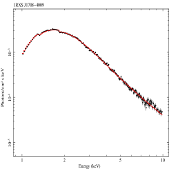
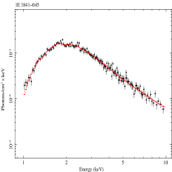
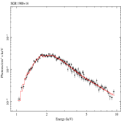
Figure 1: 1RXS J1708-4009 , 1E 1841-045 , and SGR 1900+14 : first row shows the spectra in Count/s/keV while in the second row we report the photon density plots of the modelling with the NTZ model. Only XMM–Newton  data have been used, and the fitting has been restricted to the $1-10$ keV range. See Table 1 and § 3 for details.

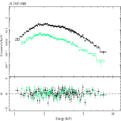
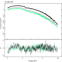
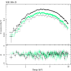
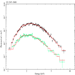
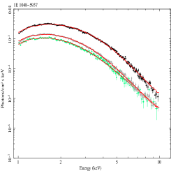
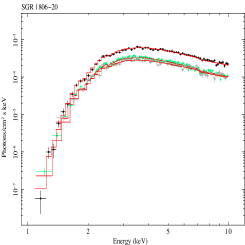
Figure 3: Same as in Fig. 1 for the AXPs 1E 1547.0-5408 , 1E 1048-5937   and for SGR 1806-20 . See Tables 2, 3 for details.

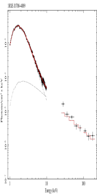
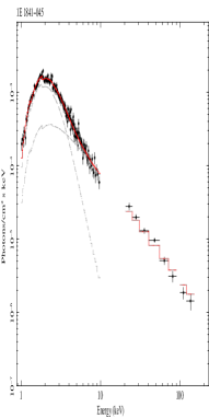
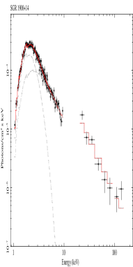
Figure 4: 1RXS J1708-4009 , 1E 1841-045 , and SGR 1900+14 : left column shows the spectra in Count/s/keV while in the right column we report the photon density plots of the modelling with the NTZ+PL model. Both XMM–Newton   and INTEGRAL   data have been used in the fitting. See Table 4 and § 3 for details.

Figure 5: Spectrum from a single emitting zone on the star surface, computed as in Nobili, Turolla & Zane (2008a, see Fig.7 in that paper and text for details). Left: The emitting area is the equatorial strip $0\leq\cos\Theta\leq 0.25$, $0\leq\Phi\leq\pi/2$. The LOS is at $\Theta_{s}=90^{\circ}$ and $\Phi_{s}=20^{\circ}$ (dotted line), $\Phi_{s}=140^{\circ}$ (dashed line) and $\Phi_{s}=220^{\circ}$ (dash-dotted line). The solid line represents the seed blackbody. Right: The emitting area is the polar cap $0.75\leq\cos\Theta\leq 1$, $0\leq\Phi\leq 2\pi$. The LOS is at $\Theta_{s}=19.5^{\circ}$ (dash-triple dotted line), $\Theta_{s}=63.5^{\circ}$ (dashed line), $\Theta_{s}=90^{\circ}$ (dash-dotted line), $\Theta_{s}=123.5^{\circ}$ (dotted line) and $\Theta_{s}=160.5^{\circ}$ (lower solid line). The upper solid line is the seed blackbody spectrum.

Figure 6: The pulsed fraction vs a measure of the surface emitting area for the AXPs in our sample; see text for details. Five more recent observations of 1E 1547.0-5408   have been also included in this plot (Bernardini et al., in preparation).

Figure 7: Combined XMM–Newton  and INTEGRAL  spectrum of SGR 1900+14 . The dashed line is the NTZ spectrum computed for the same values of parameters that best-fit the XMM–Newton  data only (see Table  1), but using the QED cross sections in the Monte Carlo code. This spectrum is than used to fit the INTEGRAL  data alone by leaving free only the value of the normalization. This gives $\chi^{2}=1.14$ for 7 d.o.f. and the ratio between the INTEGRAL  and the XMM–Newton  normalizations is 8.8. Solid line: same as before but with $\beta_{bulk}=0.61$, $kT=0.57$ keV and $\Delta\phi=0.54$; all parameters are at $3\sigma$ from their best fitting values of the XMM–Newton  spectrum. Here the reduced $\chi^{2}=1.07$ for 7 d.o.f. and the ratio between the INTEGRAL  and the XMM–Newton  normalizations is 2.8.

References

- Anders & Grevesse (1989) Anders E., & Grevesse N., 1989, Geochimica & Cosmochimica Acta 53, 197
- Baring & Harding (2007) Baring M. G., Harding A.K. 2007, Ap&SS, 308, 109
- Beloborodov (2009) Beloborodov, A.M. 2009, ApJ, submitted [arXiv:0812.4873]
- Beloborodov & Thompson (2007) Beloborodov A.M., Thompson C. 2007, ApJ, 657, 967
- Bernardini et al. (2008) Bernardini F., et al. 2009, A&A, 498, 195
- Campana et al. (2007) Campana S., Rea N., Israel G. L., Turolla R., Zane S. 2007, A&A, 63, 1047
- Den Hartog et al. (2008a) Den Hartog P.R., et al. 2008a, A&A, 489, 245
- Den Hartog et al. (2008b) Den Hartog P.R., Kuiper L., Hermsen W. 2008b, A&A, 489, 263
- Duncan & Thompson (1992) Duncan R., Thompson C. 1992, ApJ, 392, L9
- Esposito et al. (2008) Esposito P., et al., 2008, ApJ, 690, L105
- Fernandez & Thompson (2007) Fernandez R., Thompson C., 2007, ApJ, 660, 615
- Geppert, Kueker & Page (2006) Geppert U., Küker M., Page D., 2006, A&A, 457, 937
- Güver, et al. (2007) Güver T., Özel F., Göḡüş E., Kouveliotou, C. 2007, ApJ, 667, L73
- Haberl et al. (2004) Haberl F., Freyberg, M.J., Briel, U.G., Dennerl, K., Zavlin, V.E., 2004, SPIE, 5165, 104
- Hurley et al. (2005) Hurley, K., et al. 2005, Nature, 434, 1098
- Lyutikov & Gavriil (2006) Lyutikov M., Gavriil F. P. 2006, MNRAS, 368, 690
- Lodders (2003) Lodders K., 2003, ApJ, 591, 1220
- Mereghetti et al. (2005a) Mereghetti S., Götz D., Mirabel I. F., Hurley K. 2005, A&A, 433, L9
- Mereghetti et al. (2005b) Mereghetti S., et al. 2005, ApJ, 628, 938
- Mereghetti (2008) Mereghetti S., 2008, A&A Rev., 15, 225
- Nobili, Turolla & Zane (2008a) Nobili, L., Turolla, R., & Zane, S., 2008a, MNRAS, 386, 1527
- Nobili, Turolla & Zane (2008b) Nobili, L., Turolla, R., & Zane, S., 2008b, MNRAS, 389, 989
- Palmer et al. (2005) Palmer, D. M., et al. 2005, Nature, 434, 1107
- Pavan et al. (2009) Pavan, L., Turolla, R., Zane, S., & Nobili, L. 2009, MNRAS, 395, 753
- Perna & Gotthelf (2008) Perna R., Gotthelf E.V., 2008, ApJ, 681, 522
- Pons, Miralles & Geppert (2009) Pons J., Miralles J.A., Geppert, U. 2009, A&A, 496, 207
- Rea et al. (2005) Rea N., et al. 2005, MNRAS, 361, 710
- Rea et al. (2007a) Rea N., Zane S., Lyutikov M., Turolla R., 2007a, Ap&SS, 308, 61
- Rea et al. (2007b) Rea N., Turolla R., Zane S., Tramacere A., Stella L., Israel G.L., Campana R. 2007b, ApJ 661, L65
- Rea et al. (2007c) Rea N., et al. 2007c, MNRAS, 381, 293
- Rea et al. (2008) Rea N., Zane S., Turolla R., Lyutikov M., Götz D. 2008, ApJ, 686, 1245
- Thompson & Belobodorov (2005) Thompson, C., Beloborodov, A. M., 2005, ApJ 634, 565
- Thompson & Duncan (1993) Thompson C., Duncan R.C., 1993, ApJ, 408, 194
- Thompson, Lyutikov & Kulkarni (2002) Thompson C., Lyutikov M., Kulkarni S. R., 2002, ApJ, 274, 332 (TLK)
- Tiengo et al. (2008) Tiengo A., Esposito P., & Mereghetti S., 2008, ApJ, 680, L133
- Woods et al. (2004) Woods P.M., et al. 2004, ApJ, 605, 378
- Woods & Thompson (2006) Woods P.M., Thompson C. 2006, in Lewin W. H. G., van der Klis M., eds., Compact Stellar X-ray Sources, Cambridge University Press, p. 547
- Woods et al. (2007) Woods P.M. et al. 2007, ApJ, 654, 470
- Zane & Turolla (2006) Zane S., & Turolla R. 2006, MNRAS, 366, 727