A Criterion for the Critical Number of Fermions and Chiral Symmetry Breaking in Anisotropic $QED_{3}$

Abstract

By analyzing the strength of a photon-fermion coupling using basic scattering processes we calculate the effect of a velocity anisotropy on the critical number of fermions at which mass is dynamically generated in planar QED. This gives a quantitative criterion which can be used to locate a quantum critical point at which fermions are gapped and confined out of the physical spectrum in a phase diagram of various condensed matter systems. We also discuss the mechanism of relativity restoration within the symmetric, quantum-critical phase of the theory.

I Introduction

Quantum Electrodynamics (QED), the quantum theory of radiation and its interaction with matter, is a subject with far reaching impact in physics, from the calculation of the magnetic moment of the electron Schwinger (1948) to the widespread use of diagrammatic tools in every corner of theoretical physics. However, despite this long tradition as a central paradigm in physics, QED continues to confront us with many new challenges as its modern reincarnations emerge as effective theories of strongly correlated many-body problems, from quantum spin liquids to high temperature superconductivity to graphene. Back in Feynman’s day, we would have been very surprised if someone were trying to solve a relativistic problem with two speeds of light. These days, such problems are actually ubiquitous in modern theoretical physics, one example being the effective theory of low energy excitations in a correlated d-wave superconductor. That theory is equivalent to an anisotropic quantum electrodynamics in $2+1$ dimensionsFranz and Tesanovic (2001); Franz et al. (2002), in which different “speeds of light” appear naturally. Furthermore, there are other systems in which the low energy description reduces to different versions $QED_{3}$, such as various forms of quantum spin liquids Hermele et al. (2005); Saremi and Lee (2007) or the physics of graphene layers Herbut et al. (2009). All of these different problems share a common feature: they have a nodal structure that resembles a relativistic spectrum for the low energy excitations. However, a distinctive feature of the $QED_{3}$ particularly relevant for cuprate superconductors is that it contains a significant intrinsic anisotropy, which exists due to the difference between the Fermi and gap velocities ($v_{F}$, $v_{\Delta}$).

It is known that the fermionic anisotropy, $\alpha=v_{F}/v_{\Delta}$, is irrelevant in the perturbative renormalization group (RG) senseVafek et al. (2002), as long as the system is in the symmetric phase of $QED_{3}$. This is the quantum-critical phase of the theory, in which strongly interacting massless fermions acquire anomalous power-law behaviors in their various correlation functions. The anomalous dimension exponents characterizing this unusual state are universal and typically depend only on the total number of fermion flavors, $N$. This however is true only as long as $N>N_{c}$, where $N_{c}$ is the critical number of fermions at which the fermion mass is dynamically generated via the mechanism of spontaneous chiral symmetry breaking (CSB). Once CSB takes place, the fermions are gapped and confined out of the physical spectrum. This heralds a different, massive phase of the theory which typically translates to a different state in the underlying condensed matter system. The results of Ref. 7 are generally valid for arbitrary anisotropy as long as the number of fermions $N$ is sufficiently large or for small anisotropy when $N$ is greater than $N_{c}$ of the isotropic case.

Evidently, $N_{c}$ is an important number within the theory, not in the least because antiferromagnetic order in effective theories of high temperature superconductors and quantum spin liquids generically arises via the above non-perturbative phenomenon of CSB – for example, in the context of cuprates, the chiral mass generation corresponds to the onset of a spin density-wave order from within a quantum disordered d-wave superconductor Herbut (2002); Tesanovic et al. (2002) while it describes the formation of the Neél antiferromagnetic state and a whole family of other order states in the context of quantum spin liquids. Hermele et al. (2005); Saremi and Lee (2007) Unlike the exponents of the critical massless phase, however, $N_{c}$ itself is not universal. Consequently, an important question arises within the anisotropic $QED_{3}$: to what extent is the critical number of fermions, $N_{c}$, which defines the boundary between broken and unbroken chiral symmetry, affected when such anisotropy is present?

In this paper, our goal is to provide an answer to this question. Of course, ours is not the answer, for two reasons. First, since $QED_{3}$ is a strongly interacting theory its exact behavior is beyond our reach. Second, since $N_{c}$ is not universal there are actually many different $N_{c}$’s: the nominally irrelevant couplings within the $QED_{3}$ theory of a quantum disordered d-wave superconductorHerbut (2002); Tesanovic et al. (2002) are very different than those of lattice-based quantum spin liquids.Hermele et al. (2005); Saremi and Lee (2007) Furthermore, both these $N_{c}$’s are different from the intrinsic $N_{c}$ of the pure $QED_{3}$ field theory considered here (defined through Balaban-Jaffe regularization,Balaban and Jaffe (1985) for example). However, all these issues notwithstanding, even in the absence of the exact solution, it is still possible to make a rather accurate determination of the parametric dependence of $N_{c}$ on the anisotropy, once an “exact” $N_{c}$ is known for the isotropic case from a different source, say from numerical simulations. Our goal is to devise a criterion for determination of $N_{c}$ within the anisotropic $QED_{3}$ which, while not exact, still provides a rather accurate description of how the CSB boundary changes as a function of the parameters of the theory. The philosophy here is similar to the one behind the ubiquitous LindemannLindemann (1910) criterion, originally proposed to predict the melting point of a solid. While not exact, the Lindemann criterion has proven itself a remarkably accurate and useful in a wide range of situations, from classical to quantum solids, from Wigner crystals to Abrikosov vortex lattices.

To devise our criterion, we point out that mass generation is a consequence of the fermion-photon coupling strength in QED. This strength is generally renormalized from its bare value by virtual polarizability of the vacuum. Relying on this fact, we propose a natural way to measure the strength of the gauge field by focusing on the matrix element that represents processes in which one photon is exchanged between two fermions. We stipulate that the CSB and mass generation take place when this matrix element exceeds certain critical value. Within the isotropic $QED_{3}$ this is manifestly an exact statement – the only unknown is the actual value of $N_{c}$ which we can either infer from a separate calculation or borrow from numerical simulations.Hands and Thomas (2005); Thomas and Hands (2007); Strouthos and Kogut Once our “Lindemann criterion” is calibrated in this fashion, we proceed to evaluate the appropriate matrix element in the anisotropic theory and propose that the CSB takes place when this matrix element exceeds the same critical value.

Following the above procedure, our criterion allows us to derive the following main results: first, we show that $N_{c}$ is not just a function of the anisotropy $\alpha$, but also a non-monotonic function of $v_{F}$ and $v_{\Delta}$ themselves. The reason behind this peculiar behavior is the existence of a third relevant velocity in the theory, the speed of light, $c_{s}$, which naturally appears in the Maxwellian action for the gauge field. We confirm our findings for $v_{\Delta}>c_{s}$ by using the Schwinger-Dyson (SD) equation within the Pisarski approximation;Pisarski (1984) both results show the same functional dependence on $v_{\Delta}$ in this regime. Another result is that the critical number of fermions decreases even for $\alpha=1$, as long as $v_{F}=v_{\Delta}\gg c_{s}$. Thus, in the context of the $QED_{3}$ effective theory of underdoped cuprates, we generically expect a non-superconducting, non-magnetic pseudogap state to intrude prior to the emergence of antiferromagnetism as d-wave superconductor is underdoped toward half-filling.

II Criterion and Calculation

We start by defining the form of the anisotropic $QED_{3}$ Lagrangian and the main physical quantities that will be used in our calculations. The Lagrangian is

$$\mathcal{L}_{Aniso}=\sum_{l=1}^{N}\bar{\psi}_{l}v_{\mu}^{(l)}\gamma_{\mu}(i\partial_{\mu}-a_{\mu})\psi_{l}+\mathcal{L}[a_{\mu}(x)]$$ (1)

where $\bar{\psi}_{l}$ are four component spinors and $a_{\mu}$ is a gauge field. In condensed matter environment, Eq. (1) is the low energy effective theory of some strongly correlated electron system. For example, in a phase-disordered d-wave superconductor, the gauge field $a_{\mu}$ couples nodal Bogoliubov-deGennes-Dirac fermions to fluctuating quantum vortex-antivortex pairs through a Maxwellian action $\mathcal{L}[a_{\mu}(x)]$. $\gamma_{\mu}$ are the standard gamma matrices, such that $\{\gamma_{\nu},\gamma_{\mu}\}=\delta_{\mu\nu}$, and $v_{\mu}^{(l)}$ is defined as $(1,v_{F},v_{\Delta})$ and $(1,v_{\Delta},v_{F})$ for nodes $l=1,2$ respectively. Fermi and “gap” velocities, $v_{F}$ and $v_{\Delta}$, define fermionic anisotropy at each node.

To make further progress we first focus our attention on a particularly simple case: the non-interacting one ($a_{\mu}=0$). This case is equivalent to saying that the phase is rigid or that the departure point in our analysis is the fully-ordered superconducting state. In that case Eq. (1) is reduced to

$$\mathcal{L}_{Dirac}=\sum_{l=1}^{2}\bar{\psi}_{l}v_{\mu}^{(l)}\gamma^{\mu}(i\partial_{\mu}+m)\psi_{l}$$ (2)

where a mass term has been introduced only for normalization purposes. In the end our results will be robust in the $m\rightarrow 0$ limit.

The equations of motion for these non-interacting Dirac fermions are:

$$(-v_{\mu}^{(l)}\gamma^{\mu}i\partial_{\mu}+m)\psi_{l}=0$$ (3)

with $l=1,2$. From this expression it is clear that the task of solving Eq. (3) can be performed independently for each fermion flavor $1$ and $2$. Now, if we focus on $l=1$, we can reduce the anisotropic equation of motion to the isotropic one using a simple change of variables $\tau^{\prime}=\tau$, $x^{\prime}=v_{F}x$, and $y^{\prime}=v_{\Delta}y$. It is worth remarking that the intrinsic fermionic anisotropy cannot be removed in the case of the real d-wave superconductor once the gauge field is present, as can be seen from the definition of $v_{\mu}^{(l)}$.

We now outline how a typical perturbative approach for computing the effect of coupling to the gauge field works: starting from the solutions obtained for the problem in which $a_{\mu}=0$, namely $\psi_{1}(\vec{x})$ and $\psi_{2}(\vec{x})$ – both having the anisotropy encoded in their spatial oscillations – we will perturbatively introduce the field $a_{\mu}$. First, we choose our free solutions for each node in the form $\psi^{+}_{l}(\vec{x})=s_{r}(m,0)\exp(-imt)$ and $\psi^{-}_{l}(\vec{x})=t_{r}(m,0)\exp(+imt)$, where for convenience we have defined $s_{1}(m,0)=(1,0,0,0)$, $s_{2}(m,0)=(0,1,0,0)$, $t_{1}(m,0)=(0,0,1,0)$, $t_{2}(m,0)=(0,0,0,1)$. The eigenstates of Eq. (3) are then

$$\psi_{1}(x)=\sum_{\vec{p}\hskip 1.0ptr=1,2}\left(\frac{m}{VE_{\vec{p}}}\right)^{\frac{1}{2}}\left(b_{r\hskip 2.0pt\vec{p}}\bar{s}_{r}(\vec{p})e^{-i\vec{p}\cdot\vec{x}}+d_{r\hskip 2.0pt\vec{p}}\bar{t}_{r}(\vec{p})e^{i\vec{p}\cdot\vec{x}}\right)$$ (4)

where $b_{r\hskip 2.0pt\vec{p}}$ and $d_{r\hskip 2.0pt\vec{p}}$ are standard fermionic annihilation operators, while $\vec{p}$ and $r$ are the momentum and spinor indices, respectively. In the case of decoupled nodes, when $a_{\mu}=0$, all the information about the anisotropy is encoded in the exponential factor. Now, for finite momentum we can use the ansatz $\psi^{+}_{1}(\vec{x})=s_{r}(\vec{k})\exp(-i\vec{k}\cdot\vec{x}^{\prime})$ and $\psi^{-}_{1}(\vec{x})=t_{r}(\vec{k})\exp(+i\vec{k}\cdot\vec{x}^{\prime})$, where $\vec{x}^{\prime}=(\tau,v_{F}x,v_{\Delta}y)$ for node $1$. The spinors $s_{r}(\vec{k})$ and $t_{r}(\vec{k})$ can be found directly from the equation of motion

$$(\hbox to0.0pt{\hbox{$\mskip 1.0mu/$}\hss}k-m)s_{r}(\vec{k})=0 (\hbox to0.0pt{\hbox{$\mskip 1.0mu/$}\hss}k+m)t_{r}(\vec{k})=0$$ (5)

where $\hbox to0.0pt{\hbox{$\mskip 1.0mu/$}\hss}k=\gamma^{\mu}k_{\mu}$. Thus, applying $(\hbox to0.0pt{\hbox{$\mskip 1.0mu/$}\hss}k+m)$ and $(\hbox to0.0pt{\hbox{$\mskip 1.0mu/$}\hss}k-m)$ to $s_{r}(m,0)$ and $t_{r}(m,0)$ respectively we can generate the needed solutions.

Using these free fermions in the Heisenberg picture, we now introduce the gauge field by employing the well-known formal solution of the scattering matrix $S$, equivalent to:

$$S=T[\exp(-i\int d^{2+1}x\mathcal{H}_{I}(\vec{x}))]$$ (6)

where $T$ and $:$ are the time ordered operator and the normal order operation, respectively. The interaction Hamiltonian density that couples fermion fields to the gauge field is given by

$$\mathcal{H}_{I}(\vec{x})=\sum_{l=1}^{2}:\bar{\psi}_{l}v_{\mu}^{(l)}\gamma_{\mu}a_{\mu}\psi_{l}:$$ (7)

Now, as usual, we want to analyze the matrix element $<f|S|i>$, where both the final and initial state are assumed to be eigenstates of the unperturbed Hamiltonian.

Figure 1: (a) Diagramatic form of the Schwinger-Dyson equation at one loop approximation. (b) Diagram used to measure the strength of a photon.

Using the Heisenberg representation of the free fields $\psi(\vec{x})$ and the Wick’s theorem, we recognize that the only relevant diagrams are the interactions photon-fermion and fermion-fermion, the so called direct scattering and the M$\ddot{o}$ller scattering. The calculation simplifies here because, due to its fluctuating nature, the contribution of $a_{\mu}$ to the first term of the $S$ matrix expansion forces the said matrix element to vanish. Consequently, the leading contribution relevant for our purposes comes from the second order term where the contraction of $a_{\mu}(\vec{x}_{1})$ with $a_{\nu}(\vec{x}_{2})$ is nothing else but the photon propagator $D_{\mu\nu}(\vec{x}_{1}-\vec{x}_{2})$, which is the real space inverse of the polarization function

$$\Pi_{\mu\nu}=\sum_{n}\frac{N}{16v_{F}v_{\Delta}}\sqrt{k_{\alpha}g^{\left(n\right)}_{\alpha\beta}k_{\beta}}\left(g^{\left(n\right)}_{\mu\nu}-\frac{g^{\left(n\right)}_{\mu\rho}k_{\rho}g^{\left(n\right)}_{\nu\lambda}k_{\lambda}}{k_{\alpha}g^{\left(n\right)}_{\alpha\beta}k_{\beta}}\right)$$ (8)

where the diagonal nodal “metric” $g_{\mu\nu}^{\left(n\right)}$ is definedVafek et al. (2002) by $g^{\left(1\right)}_{00}=g^{\left(2\right)}_{00}=1$, $g^{\left(1\right)}_{11}=g^{\left(2\right)}_{22}=v_{F}^{2}$ and $g^{\left(1\right)}_{22}=g^{\left(2\right)}_{11}=v_{\Delta}^{2}$, and $\gamma_{\nu}^{\left(n\right)}=\sqrt{g^{\left(n\right)}_{\mu\nu}\gamma_{\mu}}$. We will now demonstrate that this second order element of the perturbation theory can be used to gainfully define the “strength” of the fermion-photon interaction and determine the critical number of fermionic flavors $N_{c}(\alpha)$, without ever solving the Schwinger-Dyson equation, even though a perturbative approach itself is condemned to failure.

In order to accomplish this, let us focus on the mass generation problem. It is well known that Schwinger-Dyson equation, Fig. 1(a), has a non trivial solution ($m>0$) once the initially soft photon (factor $1/N$ in the large $N$ limit) becomes harder at a critical number of fermions, $N_{c}$; with $3<N_{c}<5$ Pisarski (1984); Nash (1989); Appelquist et al. (1988); Hands and Thomas (2005). That means for $N<N_{c}$ mass will be dynamically generated and therefore chiral symmetry would be broken.

The existence of anisotropy makes to analyzing the birth of a gapped state through the mechanism of mass generation using the Schwinger-Dyson formalism almost impossible, with the noteworthy exception of the isotropic limit and the so called small anisotropy case ($v_{F}=1+\delta$,$v_{\Delta}=1$, where $\delta\ll 1$) Lee and Herbut (2002); Vafek et al. (2002); Stanev . Our aim is to explore mass generation for arbitrary anisotropy, because this is the physically relevant regime. Our technique is based on the observation that as we lower $N$ we are effectively making the photon interaction stronger. This is clear because the photon propagator contains a screening factor $\frac{1}{N}$. From this simple observation we can see that mass generation is a phenomenon that is intrinsically tied to the strength of the gauge field (photons).

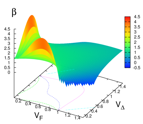
Figure 2: The calculated ratio $\beta$. The minimum value of $v_{F}$and $v_{\Delta}$ is $0.15$ and the maximum $1.5$. This graph shows that $N_{c}$ is not a simple function of $\alpha$ but a more complex function of $v_{F}$ and $v_{\Delta}$ .

Put simply, we can translate the meaning of $N_{c}$ into the following statement, which clearly is a necessary condition for mass generation: If the photon-exchange interaction is stronger than some threshold value $A_{c}$ then the fermion mass will be dynamically generated. This assertion clearly lacks the precision of a mathematical theorem but we now proceed to demonstrate that it has the practical virtue of a useful criterion.

The problem that we are facing is straightforward: How can we usefully quantify the $\it{strength}$ of the gauge field? The simplest way to measure the strength of a photon is to analyze a process in which one photon is exchanged. For the sake of simplicity, we will analyze the $\it{fermion-fermion}$ scattering mediated by one $\it{photon}$, as shown in Fig. 1(b) which corresponds to the second order term in perturbation theory. Thus using the $N_{c}$ borrowed from the isotropic limit, we define $A_{c}=<i|S^{(2)}|f>[N_{c}(\alpha=1)]$, the matrix element of the $S$ matrix evaluated at the isotropic limit, as the natural candidate to measure the strength of the photon. We can safely say that in an anisotropic theory mass will be generated at the critical strength defined by $A_{c}$.

Thus solving the equation, $A_{c}=<i|S^{(2)}|f>[N_{c}(\alpha)]$ for $N_{c}(\alpha)$, we will find the influence of anisotropy on the critical number of fermion flavors. In the isotropic case, the choice of node will not make any difference, however in the anisotropic case the situation will be quite different. Regarding the symmetries of the problem we must analyze the invariant, $<i|S^{(2)}|f>(v_{F},v_{\Delta})+<i|S^{(2)}|f>(v_{\Delta},v_{F})$ because nodal particles can be born indifferently in nodes $1$ or $2$. This quantity is invariant under the transformation $v_{F}\leftrightarrow v_{\Delta}$, which is a physical symmetry of this problem.

We now proceed to compute the first non zero matrix element $<i|S^{(2)}|f>$. The second order process following from the S-matrix term, Eq. (6) is:

$$S^{(2)}\propto T[\int\mathcal{H}_{I}(\vec{x}_{1})\mathcal{H}_{I}(\vec{x}_{2})dx_{1}dx_{2}]$$ (9)

which can be written (integration with respect to $x_{1}$ and $x_{2}$ is implicit) as a sum of terms of the type

$$T[:\bar{\psi}_{1}(x_{1})\gamma_{\mu}^{(1)}a_{\mu}(x_{1})\psi_{1}(x_{1})::\bar{\psi}_{1}(x_{2})\gamma_{\nu}^{(1)}a_{\nu}(x_{2})\psi_{1}(x_{2}):]$$ (10)

By applying Wick’s theorem to the previous expression terms with and without contractions are obtained. However, due to the fluctuating nature of the gauge field most of those terms will vanish. The survivor will be the one containing the contraction of the gauge field with itself. Thus, the problem is reduced to compute the matrix element:

$$:\bar{\psi}_{1}(x_{1})\gamma_{\mu}^{(1)}\psi_{1}(x_{1})\bar{\psi}_{1}(x_{2})\gamma_{\nu}^{(1)}\psi_{1}(x_{2})D_{\mu\nu}(x_{2}-x_{1}):$$ (11)

To evaluate such matrix element we must define the initial and final states of the system $|i>,|f>$. As the strength of the photon should be independent of the states that we use to measure it, we are free to use

$${|i>=b^{\dagger}_{r_{1}\vec{p}_{1}}b^{\dagger}_{r_{2}\vec{p}_{2}}|0>}\text{ and }{|f>=b^{\dagger}_{r^{\prime}_{1}\vec{p^{\prime}}_{1}}b^{\dagger}_{r^{\prime}_{2}\vec{p^{\prime}}_{2}}|0>}$$

which we already know from the free theory. The relevant matrix element is

$$\frac{1}{N}<i|S^{(2)}|f>(\Lambda,v_{F},v_{\Delta})\sim\frac{1}{v_{\Delta}v_{F}}\int d^{3}k\left(\frac{1}{p_{i0}(p_{i0}-k_{0})}\right)Q_{\mu}(\vec{p}_{i}-\vec{k},\vec{p}_{i})D_{\mu\nu}(g^{(1)}\vec{k})Q_{\nu}(\vec{p}_{i},\vec{p}_{i}-\vec{k})$$ (12)

where $Q_{\mu}(\vec{P},\vec{p})=\bar{s}(\vec{P})\gamma^{(1)}_{\mu}s(\vec{p})$, with $\bar{s}=s\gamma_{0}$. The integral is to be performed over all the allowed $k-space$, but we have one constraint that is the spectrum of the Dirac fermions, $k_{0}=\sqrt{\left(v_{F}k_{x}\right)^{2}+\left(v_{\Delta}k_{y}\right)^{2}}$, which allows us to further reduce the evaluation of this integral.

The integration limits are fixed from the condition that the momentum transferred in the processes shown in Fig. 1(b) can not be larger that the momentum of the incident particle, $\vec{p}_{i}$. We have set $p_{x}=p_{y}=\Lambda$ as an upper cut off. We have also verified that the only effect of choosing a different cut off for different spatial directions is that it makes the convergence slower. Thus, using the invariant measure of the strength of the gauge field, it is straightforward to show that the ratio between critical number of fermions at velocities $v_{F}$ and $v_{\Delta}$ respect to the isotropic point is

$$\beta=\frac{<i|S^{(2)}|f>(\Lambda,v_{F},v_{\Delta})+<i|S^{(2)}|f>(\Lambda,v_{\Delta},v_{F})}{2<i|S^{(2)}|f>(\Lambda,1,1)}$$ (13)

Thus, the critical number of fermions for the anisotropic theory is given by the product of, $\beta(v_{F},v_{\Delta})$, and the critical number of fermions at the isotropic point $N_{c}\left(1,1\right)$. In principle, this measure of the strength of the gauge field depends on the initial momentum of the particles, but it turns out that the ratio between the strength of the gauge field with anisotropy and the strength of the gauge field without anisotropy $\alpha=1$ is not sensitive to the momentum of the incident fermions, $\vec{p}_{i}$. In fact, all the calculated quantities converge to a fixed value for a fairly low momentum cut off, $\Lambda$. It is important to remark that $\beta$ is gauge invariant due to the transverse nature of the photon.

Indeed we can do better. By isolating the leading divergent behavior of the scattering amplitude we have obtained that in the $\Lambda\rightarrow\infty$ at the leading order in the large $N$ approximation, the ratio $\beta$ is given by:

$$\beta\left(v_{F},v_{\Delta}\right) = \zeta_{1}\left[\sqrt{1+v_{\Delta}^{2}}\mathbf{E}\left(\frac{v_{\Delta}^{2}-v_{F}^{2}}{1+v_{\Delta}^{2}}\right)+\sqrt{1+v_{F}^{2}}\mathbf{E}\left(\frac{v_{F}^{2}-v_{\Delta}^{2}}{1+v_{F}^{2}}\right)\right]+\zeta_{2}\left[\mathbf{K}\left(\frac{v_{F}^{2}-v_{\Delta}^{2}}{1+v_{F}^{2}}\right)+\mathbf{K}\left(\frac{v_{\Delta}^{2}-v_{F}^{2}}{1+v_{\Delta}^{2}}\right)\right]$$ (14)

where

$$\mathbf{E}\left(m\right)=\int_{0}^{\frac{\pi}{2}}\left[1-m\sin(\theta)\right]^{1/2}d\theta$$

$$\mathbf{K}\left(m\right)=\int_{0}^{\frac{\pi}{2}}\left[1-m\sin(\theta)\right]^{-1/2}d\theta$$ (15)

$$\zeta_{1}=-2\left(\frac{1-2\left(v_{F}^{2}+v_{\Delta}^{2}\right)-v_{F}^{2}v_{\Delta}^{2}+v_{F}^{4}+v_{\Delta}^{4}}{3\sqrt{2}\pi v_{F}^{2}v_{\Delta}^{2}}\right)$$

$$\zeta_{2}=\frac{2-3\left(v_{F}^{2}+v_{\Delta}^{2}\right)+\left(v_{F}^{2}-v_{\Delta}^{2}\right)^{2}+v_{F}^{4}v_{\Delta}^{2}+v_{\Delta}^{4}v_{F}^{2}}{3\sqrt{2}\pi v_{F}^{2}v_{\Delta}^{2}\sqrt{\left(1+v_{F}^{2}\right)\left(1+v_{\Delta}^{2}\right)}}$$

are the elliptic functions of first and second kind respectively, and the prefactors are polynomials that are symmetric under $v_{F}\leftrightarrow v_{\Delta}$. Thus $\beta$ is explicitly invariant under the transformation $v_{F}\leftrightarrow v_{\Delta}$, as it must be.

An important case is the one in which there is no $\it{fermionic}$ $\it{anisotropy}$, i.e. $v_{F}=v_{\Delta}$. In this case all the integrals can be performed and the full divergent behavior of Eq. (12) can be isolated by going to cylindrical coordinates as the $x\leftrightarrow y$ symmetry suggests. The result is just the limit behavior of Eq. (14) when taking $v_{F}=v_{\Delta}$. In that limit the dependence on the fermionic velocities becomes particularly simple.

$$\beta=\sqrt{\frac{2}{1+v_{\Delta}^{2}}}$$ (16)

To test the accuracy of our technique, the result is compared with the exact numerical integration in Fig. 3, showing excellent agreement. For low speeds $v_{\Delta}<1$, our result suggest that the critical number of fermions increases. We discuss this case in more detail below. On the opposite limit when the gauge field velocity is small compared with the other two velocities the critical number of fermions goes to zero.

Figure 3: Comparison between the numerical and analytical calculation of $\beta$ in the case for which $v_{F}=v_{\Delta}$.

A non trivial dependence on the gauge field velocity was also found; there are three different regimes depending upon the value of $v_{F}$, with respect to $c_{s}$, as shown in Fig. 2. For $v_{F}<c_{s}$, the critical number of fermions increases, reaching unexpected values for large anisotropy, leading to a gapped state in this sector. On the other hand for $v_{F}>c_{s}$, $N_{c}$ decreases and we can generically expect gapless excitations. The most unexpected result occurs if $v_{F}=c_{s}$, in this case $N_{c}(\alpha)\approx N_{c}(1)$ for $\alpha>1$. Even though we found small deviations with respect to the isotropic value near to $\alpha=2$, they do not change the integer part of $N_{c}$ (See also Fig. 5). Thus, in this regime large anisotropy will be completely irrelevant.

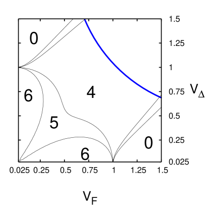
Figure 4: Phase diagram for the critical number of fermions in the velocity space. We have set the critical number of fermions for the isotropic theory at $N_{c}=4$. Inside the square defined by the lines $v_{F}=1$ and $v_{\Delta}=1$ the critical number of fermions never vanishes. The blue line corresponds to $v_{F}=1/v_{\Delta}$ and represents the one dimensional domain simulated by Thomas and HandsHands and Thomas (2005).

Using $N_{c}(1)=4$, which is the integer closest to the gauge invariant critical number of fermions $128/3\pi^{2}$ found by Nash Nash (1989), we have obtained a phase diagram in the ($v_{F}$, $v_{\Delta}$) space, Fig. 4. In this plot it is clear that if both velocities are smaller than $c_{s}$, the critical number of fermions never goes to zero. However, outside that square region $N_{c}\rightarrow 0$ for high anisotropies.

To show how important it is to consider the scale defined by $c_{s}$ we have also plotted $\beta(\alpha)$ for different values of $v_{F}$ ($0.5,1,5.0$) that we kept fixed as $v_{\Delta}$ was varied (See Fig. 5). In this plot we make evident that $c_{s}$ is a relevant parameter which we are allowed to set to $1$, however the detailed behavior of the system is not a simple function of the anisotropy, $\alpha$, but an explicit function of both parameters $v_{F}$ and $v_{\Delta}$.

In order to test our results we compare them with recent numerical work that has been done by Thomas and Hands (T-H)Hands and Thomas (2005) in an attempt to understand how anisotropy can modify the properties of $QED_{3}$. The lattice (Euclidean) version used by T-H includes an anisotropy which is intended to mimic the continuum model in the incarnation presented by Lee and Herbut Lee and Herbut (2002). The $QED_{3}$ theory presented in Lee’s article is parametrized in terms of two quantities $\delta=\sqrt{v_{F}v_{\Delta}}$ and $\lambda=v_{F}/v_{\Delta}$. T-H have used an extended lattice model similar to the one used by Dagotto et al Dagotto et al. (1989), that in the continuum limit resembles the behavior of Eq. (1). In order to perform the simulation the action used was:

$$S=\sum_{i=1}^{N}\sum_{x,x^{\prime}}a^{3}\bar{\chi}_{i}(x)M_{x,x^{\prime}}\chi_{i}(x^{\prime})+\frac{\beta}{2}a^{3}\Theta^{2}_{\mu\nu}(x)$$ (17)

where the anisotropy was introduced in the fermion matrix

$$M_{x,x^{\prime}}=\frac{1}{2a}\sum_{\mu=1}^{3}\xi_{\mu}(x)\left[\delta_{x^{\prime},x+\hat{\mu}}U_{x\mu}-\delta_{x^{\prime},x-\hat{\mu}}U^{\dagger}_{x^{\prime}\mu}\right]+m\delta_{\mu\nu}$$ (18)

and

$$\xi_{\mu}(x) = \lambda_{\mu}\eta_{\mu}(x)$$ (19)

$$\eta_{\mu}(x) = (-1)^{x_{1}+...+x_{\mu}}$$ (20)

with $x_{1}=x$, $x_{2}=y$ and $x_{3}=\tau$, is the Kawomoto-Smit phase of the staggered fermion field. The lattice spacing is $a$. An important definition is that of the anisotropy factors, $\lambda_{x}=\alpha^{-\frac{1}{2}}$, $\lambda_{y}=\alpha^{\frac{1}{2}}$ , and $\lambda_{\tau}=1$ . This definition is important for our purposes because it shows that T-H lattice theory does not keep the flavor symmetry of the model relevant for cupratesFranz and Tesanovic (2001); Vafek et al. (2002); Franz et al. (2002); Hands and Thomas (2005). Regardless this intrinsic drawback of the method we will show that it still mimic the qualitative behavior of the flavor symmetric anisotropic $QED_{3}$ at least in the low anisotropy limit.

In their numerical simulation T-H have a single parameter, which is equivalent to $\alpha=v_{F}/v_{\Delta}$, and as an extra constraint they have set $\delta=1$. This choice imply that $v_{F}=1/v_{\Delta}$ and therefore $\alpha=1/v_{\Delta}^{2}$. That means that T-H have simulated a 1-D domain of the whole parameter space $(v_{F},v_{\Delta})$. That domain is shown in Fig. 4 as a blue line. In order to make a link between the amount of condensate $<\bar{\psi}\psi>$ and its relation with $N_{c}(\alpha)$ we will assume that the functional form of the dynamically generated mass does not change Appelquist et al. (1988); Nash (1989) as we introduce anisotropy in the system. This can be explicitly checked in the small anisotropy limitStanev . As long as we are inside to the broken phase and near to the boundary between broken and unbroken phases, the mass has the following functional form

$$m=m_{o}\exp\left(\frac{-2\pi}{\sqrt{\frac{N_{c}(v_{F},v_{\Delta})}{N}-1}}\right)$$ (21)

where $m_{o}$ may depend on $N$. However, what is important is how to define the boundary between the massless phase and the massive phase. This is done by solving Eq. (21) when $m=0$. We can also interpret this equation in the following way: For a fixed number of Fermions, $N$, this equation allow us to understand how the mass changes as a function of $N_{c}(\alpha)$ when $N$ is close to $N_{c}$. In fact, for any number of fermions when $N_{c}(\alpha)=N$ it is prohibited to have any condensate. That means that the critical anisotropy $\alpha_{c}$ that solve $m(\alpha_{c})=0$ for any value of $N$ is the same that the critical anisotropy that solves $N_{c}(\alpha_{c})=N$. Hands reported that such a critical anisotropy $\alpha_{c}\approx 4$ in a $16^{3}$ sites lattice simulation which is in agreement with the critical value found by us $\alpha_{c}\approx 3$. This decreasing behavior is in contrast to the one found in Ref. 18, where it was claimed that $N_{c}$ increases as a function of the bare anisotropy. Taking into account that the lattice simulation is a non perturbative method that does not relay in any educated ansatz, T-H results strongly support our view of the phenomenon. Still, we should mention that the critical anisotropy calculated by T-H using the anisotropic scaling is not, in the strict sense, quantitatively accurate in the context of cuprates, for two reasons. First, the scaling used brakes the crystal isotropy, or, in different words, their simulation is not invariant under flavor exchange. Second, they assumed that the two fermionic velocities change little around the gauge field velocity $c_{s}=1$. Due to the collective nature of phase defects we expect that $c_{s}\ll v_{F}$ in cuprates Concha .

On the other hand lattice simulations are always performed in finite lattices and therefore the correct comparison with our results should be done by considering both, an upper cut off and a lower cut off. In principle we are free to make the upper cutoff as large as we want but the lower cut off dependence may be important when comparing our results with finite lattice simulationsGusynin et al. (1996). Setting the upper cut off as $\Lambda_{u}=1$ then the lower cut off should be $\Lambda_{d}\sim 1/L$, where $L$ is the size of the system. As we change the lower cut off we have found no significant differences in our results as it goes to zero.

Figure 5: Ratio between the critical number of fermions in the anisotropic theory and its equivalent within the isotropic theory as a function of anisotropy, $\beta(\alpha)$. The three curves represent the three regimes found: $N_{c}(\alpha)<N_{c}(1)$ if $v_{F}>1$, $N_{c}(\alpha)/N_{c}(1)$ approaches a constant $\sim 1$ if $v_{F}=1$, and $N_{c}(\alpha)$ increases for increasing $\alpha$ if $v_{F}<1$.

We have also investigated the effect of the breaking of the flavor symmetry in our scheme. For this purpose we have used only one amplitude for the photon, so that the final kernel is not invariant under $v_{F}\leftrightarrow v_{\Delta}$. In this case, we have obtained the same qualitative behavior as shown in Fig. 6, and the small negative slope at the isotropic point, detail that is in agreement with the results shown by T-H in [Fig. 5, (Ref. 11)]. This clearly is a symptom of the breaking of flavor symmetry. However, there is a very important issue that emerges once we arbitrarily break flavor symmetry. The function $\beta$ starts to pick up a phase which is unphysical. $\beta$ must be a real number as $N_{c}$ is. This makes evident that even with the simplest interaction between fermions the flavor symmetry is needed in order to obtain a meaningful value of $\beta$. This observation suggest that numerical simulations that preserve flavor symmetry are the only reliable way to extract accurate critical values. However, we must encore that the qualitative behavior of T-H simulation agrees with the physical picture proposed in this article.

Figure 6: $\beta$ within the domain defined by the blue line of Fig. 4. The continuous line represents the flavor symmetric calculation. The dotted line is the non-symmetric calculation. For the latter case we have only plotted the real part because the breaking of the flavor symmetry introduces a small but persistent imaginary part.

Looking at the obtained phase diagram, Fig. 4, the question that naturally arises is, which regime is the physically relevant one? Clearly our answer will depend on the ratio $v_{F}/c_{s}$. At finite but still small temperature, $T$, we can use the continuum vortex-antivortex Coulomb plasma model in order to estimate the gauge field velocity. Identifying the speed of light from the Maxwellian form of the action for the gauge field we find that $c_{s}\sim\sqrt{n_{l}/T}$ at finite $T$, where $n_{l}$ is the density of vortices Franz et al. (2002). Thus for any $T>0$ as we approach the superconducting state $n_{l}\rightarrow 0$ and thus $c_{s}\rightarrow 0$, resulting in a protected symmetric phase. As $n_{l}$ increases, for small but finite $T$, $c_{s}$ may reach very high values, but if those values are larger than $v_{F}$ is unclear. If we go to the line $T=0$ quantum fluctuations will drive the system into a region in which the value of $c_{s}$ will depend on the specific value of the dynamical critical exponent $z$, that in some simplified calculations was adopted to be $1$. The more striking problem about identifying the precise value of $c_{s}$ is that this velocity is a function of the correlation length, $c_{s}=f(\xi_{sc})$, but at the same time we know that $\xi_{sc}=\xi_{sc}(x,T)$, thus a self consistent treatment or knowledge of the correlation length from experiments will be needed to settle this problem and give an accurate phase diagram that identify the relevance of these different regimes.

To provide further evidence of our findings we have also re-analyzed from a different perspective the case in which $\it{fermionic}$ $\it{anisotropy}$ is one. We have applied Pisarski’s technique Pisarski (1984) to find the qualitative behavior of the dynamically generated mass as a function of $v_{\Delta}$.

We will assume that $\Sigma\left(p\right)\sim\Sigma\left(0\right)$. Thus in the appropriate integration interval $(\Sigma\left(0\right),\Lambda)$ the mass will be a constant. This assumption is certainly incorrect, as was shown by Appelquist Appelquist et al. (1988); Nash (1989) et al. However, it will allow us to compare the qualitative behavior of the mass as a function of $v_{\Delta}$, for the case in which $v_{F}=v_{\Delta}$. In this case the sums can be performed analytically by going to cylindrical coordinates instead of spherical ones. The integration was performed over the shell defined by a lower cutoff $\Sigma\left(0\right)$ and an upper cut off $\Lambda$. Thus the Schwinger-Dyson equation:

$$\Sigma_{(n)}\left(\vec{p}\right)=\int\frac{\gamma_{\mu}^{(n)}D_{\mu\nu}(\vec{p}-\vec{k})\gamma^{(n)}_{\nu}\Sigma_{(n)}(\vec{k})}{k_{\mu}g^{n}_{\mu\nu}k_{\nu}+\Sigma^{2}_{(n)}(\vec{k})}d^{3}k$$ (22)

can be solved in this rough approximation and the result is:

$$\Sigma(0)\sim\exp\left(-\frac{N\pi^{2}v_{\Delta}^{2}}{8\sqrt{v_{\Delta}^{2}-1}}\right)$$ (23)

which is a real number as long as $v_{\Delta}>1$. Thus as long as the $\it{neutrinos}$ move faster than the photons the generated mass indeed does depend on $v_{\Delta}$.

We expect that – given the fact the decay factor in Pisarski’s result is of order $N_{c}$ – the correction found for that factor will give us the functional behavior of $N_{c}(v_{\Delta})$. Thus, as $v_{\Delta}\gg 1$ we would expect that $N_{c}\sim 1/v_{\Delta}$. This is consistent with the result obtained from the proposed criterion, Eq. (16). However, we should warn the reader that even thought a mathematical expression can be obtained for $v_{\Delta}<1$ the nature of the system will change in this case, casting doubt on the validity of our criterion in that region. Indeed, from S-D equation at the Pisarski level approximation for low fermionic velocities, the self energy will acquire an imaginary part which can be interpreted as leading to a confinementMaris (1995) for fermions of the theory. This instantly calls into question the validity of using a pure plane wave type solutions for the computation of the scattering process.

In this approximation, the nature of the solution changes considerably at the point where $v_{\Delta}=1$. That is so because the radial integral gets a logarithmic contribution that is proportional to $\sqrt{1-v_{\Delta}^{2}}$ which overwhelms the leading contribution at the isotropic point. Alternatively, in more physical terms, if photons and massless fermions move at precisely the same speed this is “infinitely” different than having the photons that move faster than fermions. In the latter case it is natural to expect an “overscreening” behavior, in which constant exchange of fast photons ultimately leads to confinement. On the opposite side, with fermions moving faster than photons, we expect photons to be less effective in screening the fermions, and thus less effective in generating their mass. We have also checked that in the isotropic limit the Pisarski’s answer obtains and thus our results are not an artifact of the parametrization used.

So far, we have shown that mass generation has a non-universal behavior, which arise due to the breaking of Lorentz invariance. Thus, it is natural for a cautious reader to wonder if, once $N>N_{c}$, the renormalized effective low energy theory is in fact Lorentz invariant or not. To begin with we emphasize that the fact that $\alpha$ flows to one by itself does not guarantee that the full Lorentz invariance will emerge unless both $c_{s}$ and $v_{F}$ are set equal; this in effect acts as an extra constraint. This is shown in Fig. (7) and in Fig. (8) where it is easy to see that even thought $\alpha\rightarrow 1$ neither $v_{F}$ nor $v_{\Delta}$ converge to $c_{s}=1$ unless the above mentioned extra constaint is imposed. To show that the full Lorentz invariance is indeed restored we must prove that both fermionic velocities $v_{F}$ and $v_{\Delta}$ flow to $c_{s}=1$ independently.

It is easy to see that Lorentz invariance can still be broken even with the fermionic anisotropy set to unity. Let us assume that the bare values of the Fermi and gap velocity are equal to each other but different from the gauge field velocity, i.e. $v_{F}=v_{\Delta}$, but $v_{F}\neq c_{s}$. The Lagrangian for this simplified theory is Kaul et al. (2008); not

$$\mathcal{L}=\bar{\psi}_{1}\left\{\gamma_{0}(\partial_{\tau}+ia_{\tau})+\gamma_{1}v_{F}(\partial_{x}+ia_{x})+\gamma_{2}v_{F}(\partial_{y}+ia_{y})\right\}\psi_{1}+(1\leftrightarrow 2)+$$

$$\frac{1}{2e^{2}}\left\{\left(\frac{\partial a_{x}}{\partial y}-\frac{\partial a_{y}}{\partial x}\right)^{2}+\left(\frac{\partial a_{\tau}}{\partial x}-\frac{\partial a_{x}}{\partial\tau}\right)^{2}+\left(\frac{\partial a_{\tau}}{\partial y}-\frac{\partial a_{y}}{\partial\tau}\right)^{2}\right\}$$ (24)

By simple rescaling $\tau^{\prime}=\tau$, $x=v_{F}x^{\prime}$, $y=v_{F}y^{\prime}$, $a^{\prime}_{\tau^{\prime}}=a_{\tau}$, $a^{\prime}_{x^{\prime}}=v_{F}a_{x}$, and $a^{\prime}_{y^{\prime}}=v_{F}a_{y}$ we can transform this theory into a new theory in which the fermionic part of the action remains fully isotropic but an anisotropic Maxwellian term appears:

$$\frac{1}{2e^{2}v^{4}_{F}}\left(\frac{\partial a^{\prime}_{x^{\prime}}}{\partial y^{\prime}}-\frac{\partial a^{\prime}_{y^{\prime}}}{\partial x^{\prime}}\right)^{2}+\frac{1}{2e^{2}v^{2}_{F}}\left\{\left(\frac{\partial a^{\prime}_{\tau^{\prime}}}{\partial x^{\prime}}-\frac{\partial a^{\prime}_{x^{\prime}}}{\partial\tau^{\prime}}\right)^{2}+\left(\frac{\partial a^{\prime}_{\tau^{\prime}}}{\partial y^{\prime}}-\frac{\partial a^{\prime}_{y}}{\partial\tau^{\prime}}\right)^{2}\right\}~{}.$$ (25)

Thus, the effect of having $v_{F}\neq c_{s}$ reduces to anisotropic couplings in the Maxwellian self-action of the gauge field. We denote these couplings as $e^{2}_{\tau}\equiv e^{2}v^{4}_{F}\text{ and }e^{2}_{\perp}\equiv e^{2}v^{2}_{F}$. These two couplings can be interpreted as two anisotropic charges. Such anisotropic charges can change the value of the critical number of fermions in the original theory, as already shown in Eq. (24). In contrast, within the isotropic $QED_{3}$, the critical number of fermions does not depend on $e^{2}$. This is true as long as we have only one coupling constant, but once we introduce two different couplings this pleasing behavior is lost.

Figure 7: The RG-$\beta$ function for $v_{F}$ (in arbitrary units) computed using the same method as in Ref. 7 but without setting $v_{\Delta}=c_{s}=1$. This plot shows the parametric dependence of the fixed point on the value at which $v_{\Delta}$ is initially set in this calculation.

This simple example shows that we can restore Lorentz invariance in the fermionic part of the action at the expense of breaking the Lorentz invariance of the Maxwellian part.

To summarize, the above discussion shows that at a bare level there are two intrinsic anisotropies in this problem; $\alpha$ is the fermionic one, while $\theta=\left(e_{\tau}/e_{\perp}\right)$ is the Maxwellian one. $e_{\tau}$ and $e_{\perp}$ are the couplings in the temporal and spatial directions respectively. Thus at a bare level of the $QED_{3}$ theory relevant for the cuprates there are four coupling constants $v_{F}$, $v_{\Delta}$, $e_{\tau}$, and $e_{\perp}$. We will now show that, even though they contain anisotropy both in the fermionic and Maxwellian terms, in the large $N$ limit the relativity is ultimately restored, without any assumptions about the size of the anisotropy.

To make good on the above claim notice that the effect of fermions on photons is still described by Eq. (8). However, the gauge field stiffness is now:

$$\Pi^{(0)}_{\mu\nu}=\frac{1}{2e_{\tau}^{2}}\bar{\epsilon}_{\chi\delta\mu}\bar{\epsilon}_{\chi\lambda\nu}k_{\lambda}k_{\delta}$$ (26)

where the anisotropic Levi-Civita symbol is defined as $\bar{\epsilon}_{\tau\eta\mu}=\epsilon_{\tau\eta\mu}$, $\bar{\epsilon}_{x\eta\mu}=\theta\epsilon_{x\eta\mu}$, $\bar{\epsilon}_{y\eta\mu}=\theta\epsilon_{y\eta\mu}$. Thus, the effective Lagrangian of the theory can be written as:

$$\mathcal{L}_{Aniso}=\frac{1}{2}\left(\Pi^{(0)}_{\mu\nu}+\Pi_{\mu\nu}\right)a_{\mu}(k)a_{\nu}(-k)$$ (27)

where the effect of fermions has been introduced through the polarization function.

Figure 8: The corresponding RG-flow of $v_{F}$ and $v_{\Delta}$ when charge renormalization is not taken into account. A line of fixed points at $v_{F}=v_{\Delta}$ is apparent.

This expression allow us to find the renormalized couplings, comparing the original bare gauge field stiffness with the screened one:

$$\Pi^{(R)}_{\mu\nu}=\Pi^{(0)}_{\mu\nu}+\Pi_{\mu\nu}$$ (28)

We find that to the lowest order in $1/N$ the renormalized couplings are:

$$\left(\frac{1}{e_{\tau}^{2}}\right)_{R} = \left(\frac{1}{e_{\tau}^{2}}\right)+\frac{N}{16\bar{k}}v_{F}v_{\Delta}$$ (29)

$$\left(\frac{1}{e_{\perp}^{2}}\right)_{R} = \left(\frac{1}{e_{\perp}^{2}}\right)+\frac{N}{16}\left(\frac{1}{k^{(1)}}\frac{v_{F}}{v_{\Delta}}+\frac{1}{k^{(2)}}\frac{v_{\Delta}}{v_{F}}\right)$$ (30)

where $1/\bar{k}=1/k^{(1)}+1/k^{(2)}$, and $k^{(i)}=\sqrt{k_{\alpha}g^{(i)}_{\alpha\beta}k_{\beta}}$.

The above one loop renormalization of the anisotropic charges allows us to set up the renormalization group (RG) equations for the beta-functions describing the flow of different couplings. These equations are rather complicated and we have been able to fully solve them only numerically. However, the following result is rather simple and can be extracted in an analytic form: on general grounds we expect that the non trivial infra-red fixed point should remain once we introduce the anisotropy, even though its position in parameter space may change. In order to find the value of the renormalized couplings at the fixed point, we analyze the difference between the renormalized couplings of the Maxwellian action

$$\left(\frac{1}{e_{\tau}^{2}}-\frac{1}{e_{\perp}^{2}}\right)_{R}=\left(\frac{1}{e_{\tau}^{2}}-\frac{1}{e_{\perp}^{2}}\right)+\hskip 72.26999pt$$ (31)

$$\frac{N}{16}\left[\frac{1}{k^{(1)}}\left(v_{F}v_{\Delta}-\frac{v_{F}}{v_{\Delta}}\right)+\frac{1}{k^{(2)}}\left(v_{\Delta}v_{F}-\frac{v_{\Delta}}{v_{F}}\right)\right]$$

If we now rearrange our RG equations so as to focus on the beta-function for this difference between the renormalized charges, $\beta_{e_{\tau}-e_{\perp}}$, the above equation implies that

$$\beta_{e_{\tau}-e_{\perp}}\sim\frac{N}{16}\left[\frac{\left(v_{F}v_{\Delta}-\frac{v_{F}}{v_{\Delta}}\right)}{k^{(1)}}+\frac{\left(v_{\Delta}v_{F}-\frac{v_{\Delta}}{v_{F}}\right)}{k^{(2)}}\right]+$$

$$+~{}(\cdots)\hskip 79.49744pt~{},$$ (32)

where $(\cdots)$ can be rewritten in terms of beta-functions for all other couplings and thus must vanish at the putative fixed point. Clearly, noting that $N$ is an arbitrarily large number, and that $k^{(i)}$ share the same sign, it follows that:

$$v^{(R)}_{F}v^{(R)}_{\Delta}-\frac{v^{(R)}_{F}}{v^{(R)}_{\Delta}}=0$$ (33)

from where $v^{(R)}_{\Delta}=1$, and, given that the theory is fully invariant under the exchange $v_{F}\leftrightarrow v_{\Delta}$, it follows that $v^{(R)}_{F}=1$. Putting this information back in the flow equations it is clear that $1/e_{\tau}^{2}$ and $1/e_{\perp}^{2}$ themselves diverge with the same slope at the fixed point, and therefore their ratio $\theta=(e_{\tau}/e_{\perp})\rightarrow 1$. This result shows that Lorentz invariance is restored and thus the previous resultsVafek et al. (2002); Hermele et al. (2005); Saremi and Lee (2007) remain valid. However, we have made it clear that the physics behind the restoration of full Lorentz invariance follows a path more subtle than previously explored: at the infra-red fixed point the relativity is restored due to the interplay between the velocity and charge renormalizations, the velocity renormalization by itself being insufficient to fully restore relativity of the theory.

III Conclusions

We have proposed a simple criterion that allows an explicit computation of the critical number of fermions $N_{c}$ in a theory that contains intrinsic anisotropies. We have checked, at the Pisarski’s level approximation, that this criterion captures the functional dependence of $N_{c}(v_{\Delta})\sim 1/v_{\Delta}$ in the case in which an explicit expression can be obtained from analytic calculations.

Our criterion suggests that lattice simulations should be performed in such a way that important symmetries of the theory, namely $v_{F}\leftrightarrow v_{\Delta}$, are protected. Otherwise, there is a danger of obtaining spurious results. In lattice $QED_{3}$, it seems worthwhile to investigate the existence of a possible confined phase in the region of the parameter space where fermionic velocities are small compared with the gauge field velocity. Another venue that remains to be explored, is the possible usefulness of similar criteria for the analysis of CSB or other non perturbative phenomena in other physical systems that also feature anisotropic couplings.

Finally, we have shown that the velocity anisotropy in $(2+1)QED$ does affect the number of critical fermion flavors $N_{c}$ at which chiral symmetry is broken due to the phenomenon of mass generation, even though the large $N$ theory remains fully relativistic in its critical phase. Surprisingly, $N_{c}$ is a non-monotonic function of $v_{F}$ and $v_{\Delta}$, and, depending on the specific value of the ratio $v_{F}/c_{s}$, different regimes emerge. Our results imply that if phase fluctuations destroy the superconducting order in underdoped cuprates, we should expect a protected chirally symmetric critical phase – i.e. the pseudogap within this theory – as doping decreases, before we reach the antiferromagnetic region in the phase diagram. Details of how will this sequence take place depend on the specific value of the gauge field velocity $c_{s}$ for different compounds. We hope that our results will contribute to better understanding of the quantitative issues that surround the value of $N_{c}$ in various effective theories and motivate further research on the anisotropic incarnations of the $QED_{3}$ theory.

IV Acknowledgments

We thank T. Senthil for useful comments. This work was supported in part by the NSF grant DMR-0531159.

References

- Schwinger (1948) J. Schwinger, Phys. Rev. 73, 416 (1948).
- Franz and Tesanovic (2001) M. Franz and Z. Tesanovic, Phys. Rev. Lett. 87, 257003 (2001).
- Franz et al. (2002) M. Franz, Z. Tešanović, and O. Vafek, Phys. Rev. B 66, 054535 (2002).
- Hermele et al. (2005) M. Hermele, T. Senthil, and M. P. Fisher, Phys. Rev. B 72, 104404 (2005).
- Saremi and Lee (2007) S. Saremi and P. A. Lee, Phys. Rev. B 75, 165110 (2007).
- Herbut et al. (2009) I. F. Herbut, V. Juričić, and B. Roy, Phys. Rev. B 79, 085116 (2009), and references therein.
- Vafek et al. (2002) O. Vafek, Z. Tesanovic, and M. Franz, Phys. Rev. Lett. 85 (2002).
- Herbut (2002) I. F. Herbut, Phys. Rev. Lett. 88, 047006 (2002).
- Tesanovic et al. (2002) Z. Tesanovic, O. Vafek, and M. Franz, Phys. Rev. B 65, 180511 (2002).
- Balaban and Jaffe (1985) T. Balaban and A. Jaffe, Erice School on Mathematical Physics 207 (1985).
- Lindemann (1910) F. Lindemann, Z. Phys 11, 609 (1910).
- Hands and Thomas (2005) S. Hands and I. O. Thomas, Phys. Rev. B 72, 054526 (2005).
- Thomas and Hands (2007) I. O. Thomas and S. Hands, Phys. Rev. B 75, 134516 (2007).
- (14) C. Strouthos and J. B. Kogut, eprint arXiv/0808.2714.
- Pisarski (1984) R. Pisarski, Phys. Rev. D 29 (1984).
- Nash (1989) D. Nash, Phys. Rev. Lett. 62, 3024 (1989).
- Appelquist et al. (1988) T. Appelquist, D. Nash, and L. C. R. Wijewardhana, Phys. Rev. Lett. 60, 2575 (1988).
- Lee and Herbut (2002) D. J. Lee and I. F. Herbut, Phys. Rev. B 66, 094512 (2002).
- (19) V. Stanev, (Unpublished).
- Dagotto et al. (1989) E. Dagotto, J. B. Kogut, and A. Kocić, Phys. Rev. Lett. 62, 1083 (1989).
- (21) A. Concha, (Unpublished).
- Gusynin et al. (1996) V. P. Gusynin, A. H. Hams, and M. Reenders, Phys. Rev. D 53, 2227 (1996).
- Maris (1995) P. Maris, Phys. Rev. D 52, 6087 (1995).
- Kaul et al. (2008) R. K. Kaul, Y. B. Kim, S. Sachdev, and T. Senthil, Nat. Phys. 4, 28 (2008).
- (25) In Ref.[24] the authors claim that fermionic anisotropy goes to one, and thus they obtain the simplified model we used to show that this can be thought as a model in which there are anisotropic couplings in the Maxwellian term. Given that the number of fermions in physical systems is modest it would be interesting to analyze the consequences of having such anisotropic couplings.