A Reconnecting Flux Rope Dynamo

Abstract

We develop a new model of the fluctuation dynamo in which the magnetic field is confined to thin flux ropes advected by a multi-scale model of turbulence. Magnetic dissipation occurs only via reconnection of the flux ropes. This model can be viewed as an implementation of the asymptotic limit $R_{\mathrm{m}}\to\infty$ for a continuous magnetic field, where magnetic dissipation is strongly localized to small regions of strong field gradients. We investigate the kinetic energy release into heat, mediated by the dynamo action, both in our model and by solving the induction equation with the same flow. We find that a flux rope dynamo is an order of magnitude more efficient at converting mechanical energy into heat. The probability density of the magnetic energy release in reconnections has a power-law form with the slope $-3$, consistent with the Solar corona heating by nanoflares.

The dynamo action, i.e., the amplification of magnetic field by the motion of an electrically conducting fluid (plasma), is the most likely explanation for astrophysical magnetic fields. Evolution of magnetic field $\mathbf{B}$ embedded in a flow at a velocity $\mathbf{u}$ is governed by

$$\frac{\partial\mathbf{B}}{\partial t}=\nabla\times(\mathbf{u}\times\mathbf{B})+\widehat{\cal L}\mathbf{B},$$ (1)

where $\widehat{\cal L}$ is an operator describing magnetic dissipation. In rarefied plasmas, such as the Solar corona, hot gas in spiral and elliptical galaxies, galactic and accretion disc halos, and laboratory plasmas, an important (if not dominant) mechanism for the dissipation of magnetic field is the reconnection of magnetic lines rather than magnetic diffusion priest:2000 , the latter modeled with $\widehat{\cal L}=\eta\nabla^{2}$ (if $\eta=\mbox{const}$). Discussions of dynamos often refer to magnetic reconnection, but attempts to include any features specific of magnetic reconnection to dynamo models are very rare B96 . On the other hand, theories of magnetic reconnection rarely, if ever, refer to the dynamo action as a mechanism maintaining magnetic fields. This paper attempts to bridge the gap between the two major areas of magnetohydrodynamics by developing a dynamo model explicitly incorporating magnetic reconnections.

The nature of the dissipation mechanism is important for the dynamo action. For example, dynamo action with hyperdiffusion, $\widehat{\cal L}=-\eta_{1}\nabla^{4}$ (and with a helical $\mathbf{u}$) has larger growth rate and stronger steady-state magnetic fields than a similar dynamo based on normal diffusion Brandenburg:2002 . This is not surprising as the hyperdiffusion operator, having the Fourier dependence of $k^{4}$, rather than $k^{2}$ of the normal diffusion, has weaker magnetic dissipation at larger scales. The release of magnetic energy in smaller regions (and larger current densities) in hyperdiffusive dynamos may also lead to a higher rate of conversion of kinetic energy to heat via magnetic energy. Magnetic hyperdiffusion also appears in the context of continuous models of self-organized criticality in application to the heating of the Solar corona SOC . The aim of such models is to reproduce the observed frequency distribution of various flare energy diagnostics.

Magnetic reconnections may have an even more extreme form of the dissipation operator than the hyperdiffusion: here magnetic fields dissipate only when in close contact with each other, so that the Fourier transform of $\widehat{\cal L}$ can be expected to be negligible at all scales exceeding a certain reconnection length $d_{0}$. It is then natural to expect that dynamos based on reconnections (as opposed to those involving magnetic diffusion) will exhibit faster growth of magnetic field, more intermittent spatial distribution and stronger plasma heating. In this paper we consider dynamo action based on direct modeling of magnetic reconnection. For this purpose, we follow the evolution of individual closed magnetic loops in a model of turbulent flow (known to be a dynamo) and reconnect them directly whenever their segments come into sufficiently close contact, with appropriate magnetic field directions. As we show here, our model exhibits a power-law probability distribution of the magnetic energy release similar to that observed in the Solar corona.

Magnetic reconnection is usually modeled with the induction equation, $\widehat{\cal L}=\eta\nabla^{2}$ (perhaps including the Hall current), and magnetic dissipation is enhanced due to the development of small-scale motions and magnetic fields. This approach may or may not apply to magnetic fields concentrated into flux ropes, where magnetic energy losses are strongly reduced at large scales and, hence, more energy can be deposited at the smaller scale of order the tube radius, where reconnections occur. Our model explores this possibility. Furthermore, our model can be viewed as a numerical implementation of the limit $R_{\mathrm{m}}\to\infty$ for a continuous magnetic field, where magnetic dissipation is confined to strongly localized regions with exceptionally high magnetic field gradients.

We model the evolution of thin flux tubes, frozen into a flow, each with constant magnetic flux $\psi$. In this paper, we focus on the kinematic behavior, where the velocity field is independent of magnetic field. To ensure that $\nabla\cdot\mathbf{B}=0$, we require that our tubes always take the form of closed loops. Numerically, we discretize the loops into fluid particles and track their position and relative order (i.e., magnetic field direction) by introducing a flag denoted $P$, with $P$ increasing along a given magnetic flux tube. Initially the particles are set a small distance apart, $0.75d$, where $d$ is an arbitrary (small) constant length scale. If, during the evolution of the loops, the distance between neighboring fluid particles on a loop becomes larger than $d$, we introduce a new particle between them, as illustrated in Fig. 1. We use linear interpolation to place the new particle halfway between the old ones. The new separation between the particles is thus greater than $0.5d$ – this will be important when we consider removing particles. Thus, the spatial resolution of our model is $d$.

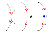
Figure 1: The algorithm for inserting new trace particles in a stretched magnetic flux tube. If the distance between any two particles (shown with open circles) exceeds a length scale $d$, a new one is inserted between them, shown with a filled circle. Labels represent magnetic field strength.

Each particle is also assigned a flag $B$ (Fig. 1) for the strength of magnetic field at that point on the loop. Assuming magnetic flux conservation and incompressability, magnetic field strength in the flux tube is proportional to its length. Magnetic field is initially constant at all particles, $B=1$. When a new particle is introduced, magnetic field is doubled, as shown in Fig. 1, at two out of three particles involved: this prescription emerged from our experimentation with various schemes and allows us to reproduce the evolution of magnetic field strength in a shear flow. Conversely, when the flow reduces the separation of particles to less than $0.5d$, we remove a particle. The value of the magnetic field strength flag is also halved on the remaining particles in a manner consistent with the above algorithm. We have verified that this prescription reproduces accurately an exact solution of the induction equation for a simple shear flow.

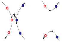
Figure 2: Reconnection occurs when the distance between two trace particles reduces to $d_{0}$ (left); the connection of the particles on a magnetic flux tube changes after the reconnection, and the two closest particles are removed (right).

If the separation between two particles, which are not neighbours, becomes less than a certain scale $d_{0}$, we reconnect their flux tubes by reassigning the flags $P$ (Fig. 2) which identify the particles ahead and those behind of those involved in the reconnection. (To obtain meaningful numerical results, $d_{0}$ has to be comparable to $d$, e.g., $d_{0}=1.5d$.) Two particles are removed from the system after each reconnection event (and their magnetic energy is lost, presumably to heat). We also monitor the cross product of magnetic fields close to the reconnection point. By ensuring that its magnitude is smaller than some tolerance $\epsilon\approx 10^{-2}$ and that the magnetic fields in the reconnecting loops are (almost) oppositely directed, we prevent parallel flux tubes with the same field direction from reconnecting. We monitor the amount of magnetic energy released in each reconnection event. To place the reconnection-based dynamo into a proper perspective, we compare it with a dynamo obtained for the same velocity field, but by solving the induction equation, i.e., Eq. (1) with $\widehat{\cal L}=\eta\nabla^{2}$. In particular, we compare the rates of magnetic energy dissipation, which can be identified with the plasma heating rate. We assume that the part of the magnetic energy which drives plasma motion at a reconnection site (such as jets) is eventually dissipated into heat as well, so that we consider that the whole magnetic energy released is converted into heat. For the induction equation, the relevant quantity is

$$\gamma_{\mathrm{i}}={d\ln M}/{dt}=\int_{V}\eta\mathbf{B}\cdot\nabla^{2}\mathbf{B}\,dV\,\left[\int_{V}\mathbf{B}^{2}\,dV\right]^{-1}\;,$$ (2)

where $M$ is the total magnetic energy. A similar quantity can be obtained for the reconnection-based dynamo by adding the contributions of all reconnection events to the magnetic energy release:

$$\gamma_{\mathrm{r}}=\frac{d\ln M}{dt}={\frac{1}{8\pi M\tau}\displaystyle\sum_{i=1}^{N_{\tau}}B_{i}^{2}S_{i}L_{i}}\;,$$ (3)

where $\tau$ is a time interval during which $N_{\tau}$ reconnections occur (we take $\tau$ to be equal to ten time steps; individual reconnection events occur in a single time step), and $B_{i}$, $S_{i}$ and $L_{i}$ are the magnetic field strength, the cross-sectional area and length of the reconnected (and thus removed) flux tube segment associated with a particle number $i$. From our assumption of frozen flux, $B_{i}S_{i}=\psi=\mbox{const}$, the total magnetic energy $M$ is,

$$M=\displaystyle\sum_{i=1}^{N_{\mathrm{tot}}}\frac{B_{i}^{2}}{8\pi}S_{i}L_{i}=\frac{\psi}{8\pi}\sum_{i=1}^{N_{\mathrm{tot}}}B_{i}L_{i}\;,$$ (4)

where $N_{\mathrm{tot}}$ is the total number of particles, and

$$\gamma_{\mathrm{r}}={\tau}^{-1}{\sum_{i=1}^{N_{\tau}}B_{i}L_{i}}\left[{\sum_{i=1}^{N_{\mathrm{tot}}}B_{i}L_{i}}\right]^{-1}\;.$$ (5)

Any comparison of the solutions of the induction equation with those from the reconnection model is not straightforward because of the difference in the control parameters of the two models: the magnetic Reynolds number $R_{\textrm{m}}=u_{0}l_{0}/\eta$ and the reconnection length $d_{0}$, respectively. A proxy for the magnetic Reynolds number can be constructed from $d_{0}$ as $\tilde{R}_{\textrm{m}}=u_{0}l_{0}/(u_{\textrm{r}}d_{0})$, where $u_{\textrm{r}}$ is the characteristic reconnection speed. The reconnection-based dynamo is significantly more efficient than the hydromagnetic dynamo, in the sense that the growth rate of magnetic field in the former is significantly larger when $R_{\textrm{m}}\approx\tilde{R}_{\textrm{m}}$. Therefore, in order to achieve conservative conclusions, we compare dynamos with similar growth rates of magnetic field. Thus, $R_{\textrm{m}}>\tilde{R}_{\textrm{m}}$ in the models compared. Magnetic field growth in a dynamo is obtained from the difference between the magnetic stretching and dissipation rates. In the reconnection-based dynamo, both are larger than those in a similar diffusion-based dynamo, but their difference is kept the same in the models which we compare below.

We consider dynamos driven by two types of flow. Firstly, this is the Kinematic Simulation (KS) model of a turbulent flow Osborne:2006 , known to be a dynamo Wilkin:2007 . Here velocity at a position $\mathbf{x}$ and time $t$ is

$${\bf u}({\bf x},t)=\sum_{n=1}^{N}\left(\mathbf{A}_{n}\times{\bf k}_{n}\cos\phi_{n}+{\bf B}_{n}\times{\bf k}_{n}\sin\phi_{n}\right),$$ (6)

where $\phi_{n}=\mathbf{k}_{n}\cdot{\bf{x}}+\omega_{n}t$, $N$ is the number of modes, $\mathbf{k}_{n}$ and $\omega_{n}=k_{n}u_{n}$ are their wave vectors and frequencies. An advantage of using this flow is that the energy spectrum, $E(k_{n})$ is controllable via appropriate choice of $\mathbf{A}_{n}$ and $\mathbf{B}_{n}$. We also note that $\nabla\cdot\mathbf{u}=0$. We adopt an energy spectrum which reduces to $E(k)\propto k^{-p}$ for $1\ll k\ll k_{N}$, with $k=1$ at the integral scale; $p=5/3$ produces the Kolmogorov spectrum, and $k_{N}$ is the cut-off scale. We have adapted (6) to periodic boundary conditions.

We also used the ABC flow of the form Childress:1995

$$\mathbf{u}=(\cos y+\sin z,\sin x+\cos z,\cos x+\sin y)\;,$$ (7)

also known to support dynamo action, to demonstrate that our results are not sensitive to the form of the flow.

\psfrag{e}[c][position=1mm]{\vspace{1mm} $\gamma_{\mathrm{i}}l_{0}/u_{0},\ \ \gamma_{\mathrm{r}}l_{0}/u_{0}$}\psfrag{t}[c][position=1mm]{\vspace{1mm} $tu_{0}/l_{0}$}\includegraphics[width=151.76964pt,height=108.405pt]{combind_energy.eps}

Figure 3: Magnetic energy release rates from the induction equation (dashed) and the flux rope model (solid). The former has a mean value of 2.4 (here $R_{\mathrm{m}}=1200$) once the eigensolution has developed. The latter (with $\tilde{R}_{\textrm{m}}=174$) has a mean value of 23 (thick horizontal line).

The initial condition is a random ensemble of closed magnetic loops, and both the induction equation and the flux rope model are evolved with the same velocity field (apart from the overall normalization to provide comparable growth rates of magnetic field). The initial condition for the induction equation is obtained by Gaussian smoothing of the magnetic field in the ropes (this procedure preserves $\nabla\cdot\mathbf{B}=0$). To evolve the induction equation, we use the Pencil Code PC:2002 on a $256^{3}$ mesh with $1000<R_{\mathrm{m}}<1500$ in a periodic box. The test particles in the flux ropes are evolved using a $4^{\textrm{th}}$ order Runge–Kutta scheme, with a time step of $l_{N}/(20u_{N})$. The algorithm for inserting and removing points is applied every time step, and the reconnection algorithm, every ten time steps. We choose $d$ to be 1/4 of the smallest length scale in the flow and set $d_{0}/d=1.5$.

Figure 3 shows the energy release rates in simulations where the growth rate of the magnetic field is $\sigma=0.16$ in both simulations (with the unit time $l_{0}/u_{0}$). The dashed line shows the energy release rate from a simulation of induction equation with $R_{\mathrm{m}}=1200$, which has the mean energy release rate $\gamma_{\mathrm{i}}\approx 2.4$. The solid line shows the corresponding results from the flux rope dynamo, with the mean value plotted as a dashed horizontal line. The mean value of the energy release rate from the reconnecting flux rope dynamo is $\gamma_{\mathrm{r}}\approx 23$, an order of magnitude larger. Also note strong fluctuations in the energy release rate from the reconnection model, which are absent in the solutions of the induction equation.

Dynamos with the ABC flow behave similarly. With $R_{\mathrm{m}}=55$, the induction equation gives an energy release rate of about $\gamma_{\mathrm{i}}=0.6$. The corresponding flux rope dynamo with the same growth rate ($0.02$) has the energy release rate of $\gamma_{\mathrm{i}}\approx 6.7$, again ten times larger.

Our approach is deliberately oversimplified with respect to the (incompletely understood) physics of magnetic reconnection. Nevertheless, we can argue that our model is conservative with respect to the reconnection efficiency. The reconnecting segments of magnetic lines in our model approach each other at a speed $u_{\mathrm{r}}\simeq u_{0}\mbox{\rm Re}^{-1/4}$ for the Kolmogorov spectrum, equal to velocity at the small scale $d_{0}\ll l_{0}$ with $l_{0}$ the energy-range scale of the flow and $d_{0}$ assumed to be close to the turbulent cut-off scale. If magnetic field is strong enough, the Alfvén speed $V_{\mathrm{A}}$, which controls magnetic reconnection in more realistic models, is of order $u(l_{0})$. Then $u_{\mathrm{r}}\ll V_{\mathrm{A}}$ and our model is likely to underestimate the efficiency of reconnections. The Sweet–Parker reconnection proceeds at a speed of order $V_{\mathrm{A}}R_{\mathrm{m}}^{-1/2}$, whereas the Petschek reconnection speed is comparable to $V_{\mathrm{A}}/\ln R_{\mathrm{m}}$ priest:2000 . For $u_{0}\simeq V_{\mathrm{A}}$ and $R_{\mathrm{m}}\simeq\mbox{\rm Re}\gg 1$, the reconnection rate in our model is larger than the former but much smaller than the latter.

\psfrag{z}[c]{\mbox{}$\log\Delta M/B_{\mathrm{rms}}^{2^{{\ }^{{\ }^{\ }}}}$}\psfrag{p}[c]{\mbox{}\vspace*{3em}Probability density}\includegraphics[height=86.72267pt]{pdf.eps}

Figure 4: Probability density for the normalized magnetic energy release in individual reconnection events, $\Delta M/B_{\mathrm{rms}}^{2}$, from the time series of Fig. 3, for the flux rope dynamo (circles) and the diffusive dynamo with the same magnetic field growth rate and velocity field form (squares). A power-law fit to the former and a Gaussian fit to the latter are shown solid and dashed, respectively.

A remarkable feature of the energy release in the rope dynamo is that its probability distribution has a power law as shown in Fig. 4, $f(x)\propto x^{-s}$, where $x=\Delta M/B_{\mathrm{rms}}^{2}$ is the magnetic energy released in a reconnection event normalized to the mean magnetic energy, with the slope $s\approx 3.3$. Importantly, the same scaling, $s\approx 3.0$, emerges when we use the ABC flow instead of KS. A similar exponent arises in a reconnection model for the corona Hughes:2003 where, however, dynamo action is not included. Thus, weak ‘flares’ dominate the energy release in our reconnection-based system, as in the nanoflare model of coronal heating P83 . Interestingly more recent results with a nonlinear adaptation of the model Baggaley:2009 retains this feature with $s\approx-3.1$ for the KS flow in the statistically steady state. We stress that the power-law behavior is not related to the self-similar nature of the velocity field: solution of the induction equation with the same velocity field, also shown in Fig. 4, has an approximately Gaussian probability distribution. It is not as yet clear if the flux rope dynamo represents a physical example of self-organized criticality, but the system does possess some of the required properties. In particular, our reconnection model has a natural threshold in terms of the current density $J>B_{\mathrm{min}}/d_{0}$, where $B_{\mathrm{min}}=1$ is the minimum magnetic field, and, as we argue above, our model can be viewed as an extreme case of magnetic hyperdiffusivity. Furthermore, our simulations are kinematic (so, magnetic energy density is assumed to be small), whereas the Solar corona is magnetically dominated. The importance of this distinction needs to be carefully investigated.

To summarize, we have confirmed that the dynamo action is sensitive to the nature of magnetic dissipation and demonstrated that magnetic reconnections (as opposed to magnetic diffusion) can significantly enhance the dynamo action. We have explored the kinematic stage of the fluctuation dynamo in a chaotic flow that models hydrodynamic turbulence and in the ABC flow, with the only magnetic dissipation mechanism being the reconnection of magnetic lines implemented in a direct manner. In our model, where magnetic dissipation is suppressed at all scales exceeding a certain scale $d_{0}$, the growth rate of magnetic field exceeds that of the fluctuation dynamo, based on magnetic diffusion, with the same velocity field. Even when the velocity field of the reconnection-based dynamo is reduced in magnitude as to achieve similar growth rates of magnetic energy density, the rate of conversion of magnetic energy into heat in the reconnection dynamo is a order of magnitude larger than in the corresponding diffusion-based dynamo. Thus, reconnections more efficiently convert the kinetic energy of the plasma flow into heat, in our case with the mediation of the dynamo action. This result, here obtained for a kinematic dynamo, can have serious implications for the heating of rarefied, hot plasmas where magnetic reconnections dominate over magnetic diffusion (such as the corona of the Sun and star, galaxies and accretion discs). In contrast to the fluctuation dynamo based on magnetic diffusion, the probability distribution function of the energy released in the flux rope dynamo has a power law form not dissimilar to that observed for the Solar flares.

We are grateful to P. H. Diamond, R. M. Kulsrud, A. Schekochihin and A. M. Soward for useful discussions and suggestions. AS is grateful to IUCAA for financial support and hospitality.

References

- (1) E. Priest and T. Forbes, Magnetic Reconnection, Cambridge University Press, 2000.
- (2) E. G. Blackman, Phys. Rev. Lett. 77, 2694 (1996).
- (3) A. Brandenburg and G. R. Sarson, Phys. Rev. Lett. 88, 055003 (2002).
- (4) P. Charbonneau, S. W. et al. Solar Phys. 203, 321 (2001).
- (5) D. Osborne et al., Phys. Rev. E 74, 036309 (2006).
- (6) S. L. Wilkin et al., Phys. Rev. Lett. 99, 134501 (2007).
- (7) S. Childress and A. Gilbert, Stretch, Twist, Fold: The Fast Dynamo, Springer, Berlin, 1995.
- (8) A. Brandenburg, Comp. Phys. Comm. 147, 471 (2002).
- (9) D. Hughes et al., Phys. Rev. Lett. 90, 131101 (2003).
- (10) E. N. Parker, Astrophys. J. 264, 642 (1983).
- (11) A. W. Baggaley, C. F. Barenghi, A. Shukurov, and K. Subramanian, Astron. Nachr 331 (2010).