Nonlinear effect on quantum control for two-level systems

Abstract

The traditional quantum control theory focuses on linear quantum system. Here we show the effect of nonlinearity on quantum control of a two-level system, we find that the nonlinearity can change the controllability of quantum system. Furthermore, we demonstrate that the Lyapunov control can be used to overcome this uncontrollability induced by the nonlinear effect.

Quantum control theory is about the application of classical and modern control strategy to quantum systems. It has generated increasing interest in the last few years due to its potential applications in metrologywiseman95 ; berry01 , communicationsgeremia04a ; jacobs07 and other technologies ahn02 ; hopkins03 ; geremia04b ; sarovar04 ; steck04 , as well as its theoretical interest. As the effective combination of control theory and quantum mechanics, the quantum control theory is not trivial for several reasons. For classical control, feedback is a key factor in the control design, and there has been a strong emphasis on robust control of linear systems. Quantum system in feedback control, on the other hand, can not usually be modeled as linear control systems, except when both the system and the controller as well as their interaction are linear. In fact for many quantum systems, the nonlinear effects can not be negligible, and in some cases they dominate the dynamics of quantum system. Moreover, feedback control requires measurement of an observable and returns the measured result as a control back to the quantum system. This renders the dynamics of the quantum system both nonlinear and stochastichabib06 . In special cases the resulting evolution can be mapped into a linear classical system driven by Gaussian noise, and consequently the optimal control problem can be solved by classical control theory. However, most control problems for such a quantum system can not be solved in this way. Therefore a study on nonlinear effects in quantum control theory is highly desired.

Lyapunov functions have played a significant role in control design. Originally used in feedback control to analyze the stability of the control system, Lyapunov functions have formed the basis for new control design. Several papers have be published recently to discuss the application of Lyapunov control to quantum systemsvettori02 ; ferrante02 ; grivopoulos03 ; mirrahimi04 ; mirrahimi05 ; altafini07 ; wang08 . Although the basic mathematical formulism is well established, many questions remain when one uses the Schrödinger equation or the master equation to describe the dynamics of quantum system, for example the nonlinear effect in quantum control.

In this paper, we shall address this issue by analyzing a two-level system with nonlinear effect. Before studying the nonlinear effect in quantum control on the two-level system, we recall that a linear two-level system is controllable by two independent parameters, then we show that nonlinear interactions may turn the controllable two-level system into uncontrollable one. This nonlinear effect may result from feedback control, and the uncontrollability can be overcome by Lyapunov control as we shall show.

Consider a two-level system described by,

$$H=\frac{R}{2}\sigma_{z}+\frac{v}{2}\sigma_{x},$$ (1)

where $\sigma_{x}$ and $\sigma_{z}$ are Pauli matrices. This model was proposed to describe the tunneling of quantum system in a double-well potential. In this model, $v$ is the coupling constant of the two wells. $R$ denotes the energy difference between the two levels. We first show that this system is controllable by manipulating the two independent parameters $R$ and $v$. The controllability requires all initial states in the Hilbert space ${\cal H}_{s}$ of the system can evolve to an arbitrary pure target state. This requirement for the initial state can be partially lifted by requiring that the Hamiltonian $H$ is unchanged up to $R$ and $v$ under the following unitary transformationyi08 ,

$$F=\left(\begin{array}[]{cc}\cos\theta&\sin\theta e^{-i\phi}\\ -\sin\theta e^{i\phi}&\cos\theta\\ \end{array}\right),$$ (2)

where $0\leq\phi\leq 2\pi,$ $0\leq\theta\leq\pi.$ By unchanged we mean $H^{\prime}=H(R^{\prime},v^{\prime})=F^{\dagger}HF$, namely the transformation $F(\theta,\phi)$ changes the control parameter in the Hamiltonian $H$ only. The proof is straightforward. Consider the Schrödinger equation $i\hbar\frac{\partial}{\partial{t}}|\varphi(t)\rangle=H|\varphi(t)\rangle,$ where $|\varphi(t)\rangle$ is the wavefunction of the system. By the time-independent transformation $F(\theta,\phi)$ , $|\varphi(t)\rangle\rightarrow{F|\phi{{}^{\prime}}(t)\rangle}$ we find $i\hbar\frac{\partial}{\partial{t}}(F|\phi{{}^{\prime}}(t)\rangle)=H(F|\phi{{}^{\prime}}(t)\rangle),$ and $i\hbar\frac{\partial}{\partial{t}}|\phi{{}^{\prime}}(t)\rangle=F^{\dagger}HF|\phi{{}^{\prime}}(t)\rangle.$ Since $H(R^{\prime},v^{\prime})=F^{\dagger}H(R,v)F$, we claim that there exists a one-to-one correspondence in sets $\{|\phi{{}^{\prime}}(t)\rangle\}$ and $\{|\varphi(t)\rangle\}.$ Therefore, if $\{|\phi{{}^{\prime}}(t)\rangle\}$ covers all (pure) states in ${\cal H}_{s}$, $\{|\varphi(t)\rangle\}$ is a convex set of all possible (pure) states for the two-level system. This observation tells us that if the system initially prepared in state $|e\rangle$ can be controlled to evolve to an arbitrary target state driven by the Hamiltonian $H^{\prime}=H(R^{\prime},v^{\prime})=F^{\dagger}H(R,v)F$, the system is controllable.

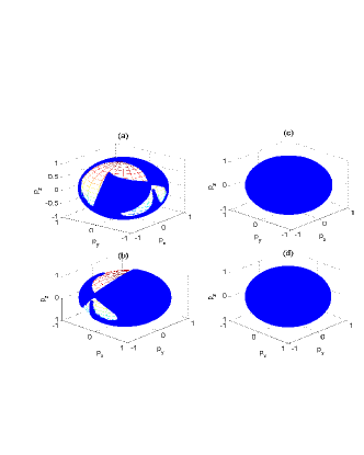
Figure 1: (color online) Accessible states (blue points on the Bloch sphere) of a two-level system driven by Hamiltonian Eq.(1) in a time interval $t\in[0,0.5]$ for (a) and (b), and $t\in[0,4]$ for (c) and (d). The parameters $R$ and $v$ both range from 0 to 7. The initial state is chosen to be $|e\rangle.$ All parameters are dimensionless. (a) and (b) [(c) and (d)] are the same but show the results from the opposite direction. $\vec{p}=(p_{x},p_{y},p_{z})$ is the Bloch vector, and $\theta=\phi=0.$

This exactly the case as shown in Fig.1, where we plot the accessible states represented by the Bloch vector $\vec{p}=(p_{x},p_{y},p_{z}).$ The Bloch vector is connected to an arbitrary state $|\varphi(t)\rangle=a(t)|e\rangle+b(t)|g\rangle$ of the two-level system through $\rho=|\varphi(t)\rangle\langle\varphi(t)|=\frac{1}{2}+\frac{1}{2}\overrightarrow{p}\cdot\overrightarrow{\sigma}$ with $p_{z}=2|a(t)|^{2}-1$, $p_{x}=a^{*}(t)b(t)+b^{*}(t)a(t),$ and $p_{y}=i(a(t)b^{*}(t)-b(t)a^{*}(t)).$ We find from Fig.1 that by varying the parameters $R$ and $v$, the two-level system indeed can evolve to an arbitrary target pure state, provided the evolution time is long enough and there is a wide range of parameters $R$ and $v$ to manipulate. It is worth addressing that the Hamiltonian in Eq.(1) becomes $H^{\prime}=\frac{R^{\prime}}{2}\sigma_{z}+\frac{v^{\prime}}{2}\sigma_{x}+\frac{u^{\prime}}{2}\sigma_{y}$ after the unitary transformation $F(\theta,\phi),$ where $R^{\prime}$ (or $v^{\prime}$) is a function of $R,v,\theta,$ and $\phi.$ $u^{\prime}$ is in general not zero. At first sight, $H$ does not satisfy the condition $H(R^{\prime},v^{\prime})=F^{\dagger}HF,$ then the two-level system driven by Hamiltonian Eq.(1) is uncontrollable. This is not the case, however, because there are only two independent parameters ($R$ and $v$) in the Hamiltonian, hence $u^{\prime}$ is not independent and may be treated as a constant. Therefore the term with $u^{\prime}$ in $H^{\prime}$ plays no role in the control on the two-level systemschirmer01 ; fu01 .

Now we study the effect of nonlinearity on the controllability of the system. For this goal, we consider a nonlinear two-level model,

$$H_{nl}=\frac{R}{2}\sigma_{z}-\frac{C}{2}\langle\psi|\sigma_{z}|\psi\rangle\sigma_{z}+\frac{v}{2}\sigma_{x},$$ (3)

where $|\psi\rangle=|\psi(t)\rangle=\left(\begin{array}[]{c}a(t)\\ b(t)\\ \end{array}\right)$ and the parameter $C$ characterizes the nonlinear interaction strength, and the other parameters have the same notations as in Eq.(1). This model can be used to describe the tunneling of Bose-Einstein condensates in a double-well potential and was widely used to study the self-trapping and tunneling in those systems.

By the unitary transformation $F(\theta,\phi)$, the Hamiltonian $H_{nl}$ is transformed into,

$$H^{{}^{\prime}}_{nl} = F^{{\dagger}}H_{nl}F,$$ (4)

$$H^{{}^{\prime}}_{nl} = (\frac{R_{nl}}{2}\cos^{2}\theta-v\cos\theta\sin\theta\cos\phi-\frac{R_{nl}}{2}\sin^{2}\theta)\sigma_{z}$$ (5)

$$+ (\frac{v}{2}\cos^{2}\theta+R_{nl}\cos\theta\sin\theta\cos\phi-\frac{v}{2}\sin^{2}\theta\cos 2\phi)\sigma_{x}$$

$$+ (R_{nl}\cos\theta\sin\theta\sin\phi-\frac{v}{2}\sin^{2}\theta\sin 2\phi)\sigma_{y},$$

where $R_{nl}=R-C\langle\psi|\sigma_{z}|\psi\rangle.$ We have performed extensive numerical simulations for the Schrödinger equation $i\hbar\frac{\partial}{\partial t}|\psi\rangle=H^{\prime}_{nl}|\psi\rangle$ with $\theta=\phi=0,$ select results are presented in Fig.2.

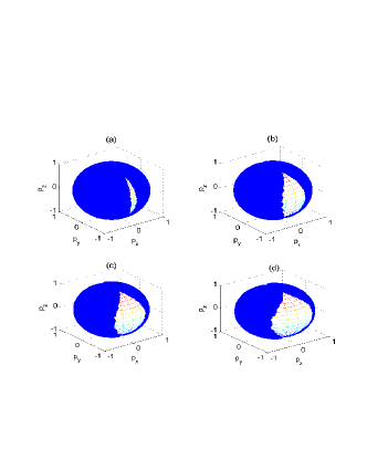
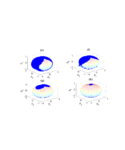
Figure 2: (color online) Effect of nonlinearity on the accessible states (blue points on the Bloch sphere) of a two-level system driven by Eq.(3) in a time interval $t\in[0,4].$ Both $R$ and $v$ range from 0 to 7. The axes $p_{x},p_{y},p_{z}$ are the Bloch vectors. The initial state is $|e\rangle$, i.e., $p_{z}=1,p_{x}=p_{y}=0,$ and $\theta=\phi=0.$ Note that there is a set of unaccessible states on the other side of the Bloch sphere, which can not be seen from this angle. (a) $C=2,$ (b) $C=6,$ (c)$C=8,$ (d) $C=10,$ (e)$C=12,$ (f)$C=14,$ (g)$C=20$ and (h)$C=100.$

Two observations can be made from Fig. 2. (1) The nonlinearity affects the controllability of the two-level system, regardless of how small the nonlinear coupling constant $C$ is, (2) the larger the nonlinear term is, the smaller the set of the accessible states. Further numerical simulation shows that $\theta$ and $\phi$ (determining the initial state) can change the accessible set of states but not the two observations, this is shown in Fig.3.

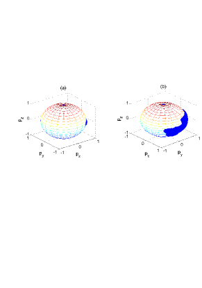
Figure 3: (color online) The same as Fig.2, but with $\theta=\pi/4,\phi=0.$ $C=20$ was chosen for this plot. (a) is the same as (b), except the position of axes $p_{x}$ and $p_{y}$.

The nonlinearity in nonlinear quantum system may come from feedback control $\frac{C}{2}\langle\psi|\sigma_{z}|\psi\rangle\sigma_{z}$. This feedback control may be understood as applying a pulse to shift the energy level of the quantum system, the amplitude of the pulse is proportional to a detection event with a rate $C$ described by $\langle\psi|\sigma_{z}|\psi\rangle$. To overcome the uncontrollability induced by the feedback, we introduce a Lyapunov control $f(t)$ to replace the coupling constant $C$ in the nonlinear term $\frac{C}{2}\langle\psi|\sigma_{z}|\psi\rangle\sigma_{z}.$ The Lyapunov control may be designed according to the Lyapunov control theory as followswang08 . For a two-level system, its Hamiltonian can be rewritten as,

$$H_{nl}=H_{0}+f(t)H_{1},$$ (7)

where $H_{0}$ is the free evolution Hamiltonian and $H_{1}$ is the control Hamiltonian. The general control task we consider can be formulated as, given a target state $|\psi_{d}(t)\rangle$, we wish to apply a certain control field $f(t)$ to the system that modifies its dynamics such that $|\psi(t)\rangle\rightarrow|\psi_{d}(t)\rangle$ as $t\rightarrow\infty.$ Since the free Hamiltonian can in general not be turned off, it is natural to assume $|\psi_{d}(t)\rangle$ to be time-dependent and satisfies

$$i\hbar\frac{\partial}{\partial t}|\psi_{d}(t)\rangle=H_{0}|\psi_{d}(t)\rangle.$$ (8)

Since the evolution of both $|\psi(t)\rangle$ and $|\psi_{d}(t)\rangle$ are unitary in our case, we can define a function

$$V[|\psi_{d}(t)\rangle,|\psi(t)\rangle]=1-|\langle\psi_{d}(t)|\psi(t)\rangle|^{2}$$ (9)

to measure the distance between the resulting and target states. Clearly $V\geq 0$ with equality only if $|\psi_{d}(t)\rangle=|\psi(t)\rangle$. Taking derivative of $V$ with respect to time $t$, we have ($|\psi_{d}\rangle=|\psi_{d}(t)\rangle$ and $|\psi\rangle=|\psi(t)\rangle$ hereafter)

$$\dot{V}=-2f(t)\mbox{Im}(\langle\psi_{d}|H_{1}|\psi\rangle\langle\psi|\psi_{d}\rangle),$$ (10)

where $\mbox{Im}(...)$ denote the imaginary part of $(...).$ So when we choose $f(t)=\kappa\mbox{Im}(\langle\psi_{d}|H_{1}|\psi\rangle\langle\psi|\psi_{d}\rangle)$ with a rate $\kappa>0$, we have $\dot{V}\leq 0.$ Therefore $V$ is a Lyapunov function for the following dynamical system,

$$i\hbar\frac{\partial}{\partial t}|\psi\rangle = H_{nl}|\psi\rangle,$$

$$i\hbar\frac{\partial}{\partial t}|\psi_{d}\rangle = H_{0}|\psi_{d}\rangle,$$

$$f(t) = \kappa\mbox{Im}(\langle\psi_{d}|H_{1}|\psi\rangle\langle\psi|\psi_{d}\rangle).$$ (11)

For a two-level system, $|\psi_{d}\rangle$ always can be written as $|\psi_{d}\rangle=c(t)|e\rangle+d(t)|g\rangle$ with $|c(t)|^{2}+|d(t)|^{2}=1$, and $|\psi\rangle=a(t)|e\rangle+b(t)|g\rangle$ with $|a(t)|^{2}+|b(t)|^{2}=1.$ When the control Hamiltonian takes $H_{1}=\sigma_{z}/2$, it is easy to find that the Lyapunov control $f(t)=-2\kappa\mbox{Im}(cd^{*}a^{*}b).$ In the following, we shall focus on the control Hamiltonian $H_{1}=\frac{1}{2}\langle\psi|\sigma_{z}|\psi\rangle\sigma_{z},$ which yields the Lyapunov control

$$f(t) = -\kappa m\mbox{Im}[(ac^{*}+bd^{*})(a^{*}c-b^{*}d)],$$

$$m = |a|^{2}-|b|^{2},$$ (12)

where we omitted the argument $t$ of $a(t),b(t),c(t)$ and $d(t)$ to shorten the notations. Clearly, the Lyapunov control renders the dynamics of the quantum system nonlinear even if the control Hamiltonian is linear. We have performed extensive numerical simulations for the dynamics of these nonlinear system, the numerical simulations show that the two-level system described by Eq.(1) with Lyapunov control $f(t)$ is controllable, namely an arbitrary pure state is accessible driven by

$$H_{nl}=\frac{R}{2}\sigma_{z}+\frac{v}{2}\sigma_{x}-\frac{f(t)}{2}\langle\psi|\sigma_{z}|\psi\rangle\sigma_{z}.$$ (13)

Then a natural question arises for $\kappa,$ how does the rate $\kappa$ in Lyapunov control $f(t)$ affect the accessible set of states?

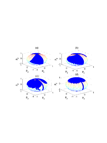
Figure 4: (color online) Accessible states represented by the Bloch vector $\vec{p}=(p_{x},p_{y},p_{z})$. The two-level system is driven by Eq.(13) with Lyapunov feedback control $f(t)$ evolving in a time interval $t\in[0,4]$ with $\theta=\phi=0$. $R$ and $v$ range from 0 to 0.5. (a) $\kappa=0$, (b) $\kappa=3$, (c) $\kappa=9$, (d) $\kappa=27$.

Fig. 4 shows the sets of accessible state reached by controlling the parameter $R$ and $v$ in a small range. In other words, the control parameters $R$ and $v$ are restricted in a regime much smaller than that by which the two-level system is controllable. We find that the rate $\kappa$ affects the accessible states. For $\kappa$ below a critical value $\kappa_{c}$, the larger the $\kappa$ is, the bigger the set of accessible states. For $\kappa>\kappa_{c},$ the situation changes, smaller $\kappa$ favors the set of accessible states. In Fig.5, we plot the short-time behavior of the accessible states, observations similar to Fig.4 can be found. A common feature we find from Fig.4 and 5 is that as $\kappa$ increases, states near the initial state $|e\rangle$ become easy to access. This finding depends on $\theta$ and $\phi.$ Finally, we address the convergence for the control system. By the Lasalle’s invariance principlelasalle61 , the largest invariant set is empty, so there is not any invariant set for the problem under consideration. The reason is that we choose $|\psi_{d}(t=0)\rangle=|\psi(t=0)\rangle$ throughout this paper.

Figure 5: (color online) The same as Fig.4, but the time interval is $[0,0.3]$, and $R$ and $v$ vary in $[0,7]$. (a) $\kappa=0$, (b) $\kappa=9$, (c) $\kappa=81$, (d) $\kappa=243$.

In summary, we have investigated the nonlinear effect on the controllability of a two-level system. This nonlinear effect can turn a controllable quantum system uncontrollable. The accessible set of states under nonlinear effect depends on the nonlinear coefficient $C$ and the initial state. To overcome this uncontrollability induced by the nonlinear effect, we propose to use Lyapunov control to manipulate the two-level system, Lyapunov function for the control system is constructed and the dependence of accessible set of states, which can be reached in a short-time limit and within a small range of control parameters on the rate $\kappa$ are shown and discussed. This study suggests that feedback control that can induce nonlinear effect changes the controllability of quantum system, Lyapunov control is better in this case for manipulating a quantum system.

This work was supported by NSF of China under Grant No. 10775023.

References

- (1) H. M. Wiseman, Phys. Rev. Lett. 75, 4587(1995).
- (2) D. W. Berry, H. M. Wiseman,and J. K. Breslin, Phys. Rev. A 63 053804,(2001).
- (3) K. Jacobs, Quant. Information Comp.7, 127(2007).
- (4) J. M. Geremia, Phys. Rev. A 70, 062303(2004).
- (5) C. Ahn, A. C. Doherty, and A. J. Landahl, Phys. Rev. A 65, 042301(2002).
- (6) A. Hopkins, K. Jacobs, S. Habib, and K. Schwab, Phys. Rev. B 68, 235328(2003).
- (7) M. Sarovar, C. Ahn, K. Jacobs, and G. J. Milburn, Phys. Rev. A 69, 052324 (2004).
- (8) D. A. Steck, K. Jacobs, H. Mabuchi, T. Bhattacharya, and S. Habib, Phys. Rev. Lett.92, 223004(2004).
- (9) J. M. Geremia, J. K. Stockton, and H. Mabuchi, Science 304, 270(2004).
- (10) S. Habib, K. Jacobs, and K. Shizume, Phys. Rev. Lett. 96, 010403(2006).
- (11) P. Vettori, in Proceedings of the MTNS Conferene, 2002.
- (12) A. Ferrante, M. Pavon, and G. Raccanelli, in Proceedings of the 41st IEEE Conference on Decision and Control, 2002.
- (13) S. Grivopoulos and B. Bamieh, in Proceedings of the 42nd IEEE Conference on Decision and Control, 2003.
- (14) M. Mirrahimi and P. Rouchon, in Proceedings of IFAC Symposium LOLCOS 2004; In Proceedings of the International Symposium MTNS 2004.
- (15) M. Mirrahimi and G. Turinici, Automatica 41, 1987(2005).
- (16) C. Altafini, Quantum Information Processing 6, 9(2007).
- (17) X. Wang and S. Schrimer, arXiv: 0801.0702; arXiv: 0901.4515.
- (18) J. Nie, H. C. Fu, and X. X. Yi, arXiv: 0805.0057.
- (19) S. G. Schirmer, H. Fu, and A. I. Solomon, Phys. Rev. A 63, 063410(2001).
- (20) H. Fu, S. G. Schirmer, and A. I. Solomon, J. Phys. A 34, 1679(2001).
- (21) J. Lasalle and S. Lefschetz, Stability by Liapunov’s Direct Method with Applications (Academic Press, New York, 1961).