Entanglement of spin chains with general boundaries and of dissipative systems

Abstract

We analyze the entanglement properties of spins (qubits) close to the boundary of spin chains in the vicinity of a quantum critical point and show that the concurrence at the boundary is significantly different from the one of bulk spins. We also discuss the von Neumann entropy of dissipative environments in the vicinity of a (boundary) critical point, such as two Ising-coupled Kondo-impurities or the dissipative two-level system. Our results indicate that the entanglement (concurrence and/or von Neumann entropy) changes abruptly at the point where coherent quantum oscillations cease to exist. The phase transition modifies significantly less the entanglement if no symmetry breaking field is applied and we argue that this might be a general property of the entanglement of dissipative systems. We finally analyze the entanglement of an harmonic chain between the two ends as function of the system size.

I Introduction

Coherence, decoherence and the measurement process are longstanding problems of quantum mechanics since they mark the fundamental difference to classical systems. They have gained increasing importance in the context of quantum computing because the operation of a quantum computer requires a careful control of the interaction between the system and its macroscopic environment. The resulting entanglement between the system’s degrees of freedom and the reservoir has been a recurrent topic since the formulation of quantum mechanics, as it is relevant to the analysis of the measurement process Omnès (1992); Zurek (2003); Amico et al. (2008).

Theoretical research on Macroscopic Quantum Tunneling lead, among other results, to the (re)formulation of a canonical model for the analysis of a quantum system interacting with a macroscopic environment, the so called Caldeira-Leggett model Caldeira and Leggett (1983a), initially introduced by Feynman and VernonFeynman and Vernon (1963). It can be shown that this canonical model describes correctly the low energy features of a system which, in the classical limit, undergoes Ohmic dissipation (linear friction). It can be extended to systems with more complicated, non-linear, dissipative properties, usually called sub-Ohmic and super-Ohmic, see below Leggett et al. (1987); Weiss (1999).

In relation to the ongoing research on entanglement, a recent interesting development is the analysis of the concurrence of spin-chains like the transverse Ising model and the XY model. It was found that the derivative of the concurrence obeys universal scaling relations close to the quantum critical point and eventually diverges at the transition Osterloh et al. (2002); Osborne and Nielsen (2002). Also other models which exhibit a quantum phase transition were subsequently investigated in this direction, as e.g. the Lipkin-Meshkov-Glick model Vidal et al. (2004); Dusuel and Vidal (2005).

Originally, the concurrence as measure of entanglement was introduced by Wooters Wootters (1998) due to its accessibility. Alternatively, the von Neumann entropy of macroscopic (contiguous) subsystems can be used Verstraete et al. (2004a). A non-local measure of entanglement was employed in the study of the Affleck-Kennedy-Lieb-Tasaki (AKLT) model Vidal et al. (2003); Verstraete et al. (2004b).

In this paper, we will first discuss the effect of boundaries of the Ising model on the entanglement properties using the concurrence as measure of entanglement. We will then discuss a model which exhibits a boundary phase transition, i.e., two Ising spins which are coupled to two Kondo impurities. This model can be mapped onto the spin-boson model and the concurrence can be computed which was originally defined for the two Ising spins at the boundary Stauber and Guinea (2004). We will then discuss various dissipative systems and compute the von Neumann entropy, focusing the discussion on the cross-over from coherent to incoherent oscillations Stauber and Guinea (2006).

The von Neumann entropy is a more general information measure than the concurrence since the latter can only be defined for two spin-1/2 systems. The former can further be generalized to a measure which relates non-contiguous sub-systems which shall be done in the third part of this paper in the context of an harmonic chain. We note by passing that the concurrence is an essentially local measure which yields zero for all spin pairs which are not nearest or next-nearest neighbors.

We close the introduction with some general remarks. The models studied here, i.e., also the spin chains, can be interpreted as quantum systems characterized by a small number of degrees of freedom coupled to a macroscopic reservoir. These models show a crossover between different regimes, or even exhibit a quantum critical point. As this behavior is induced by the presence of a reservoir with a large number of degrees of freedom, they can also be considered as a model of dephasing and loss of quantum coherence. It is worth noting that there is a close connection between models describing impurities coupled to a reservoir, and strongly correlated systems near a quantum critical point, as evidenced by Dynamical Mean Field Theory Georges et al. (1996). In the limit of large coordination, the properties of an homogeneous system can be reduced to those of an impurity interacting with an appropriately chosen reservoir. Hence, in the limit of large coordination the entanglement between the quantum system and the reservoir near a phase transition can be mapped onto the entanglement which develops in an homogeneous system near a quantum critical point.

II Concurrence of the Ising model with general boundaries

II.1 The transverse Ising model

We start with the homogeneous, one-dimensional transverse Ising model with open boundary conditions and coupling parameter $\lambda$. The two spins at the end are further connected by an additional coupling parameter $\kappa$. For $\kappa=\lambda$, one recovers the Ising model on a ring. The full Hamiltonian thus reads

$${\cal H}=-\lambda\sum_{i=1}^{N-1}\sigma_{i}^{x}\sigma_{i+1}^{x}-\sum_{i=1}^{N}\sigma_{i}^{z}-\kappa\sigma_{1}^{x}\sigma_{N}^{x}\;,$$ (1)

where $\sigma_{i}^{x,z}$ are the $x,z$-components of the Pauli matrices.

To solve the model one first converts all the spin matrices into spinless fermions $c_{i}$ with $\{c_{i},c_{i^{\prime}}^{\dagger}\}=\delta_{i,i^{\prime}}$ Lieb et al. (1961); Pfeuty (1970). This is done by performing a Jordan-Wigner transformation

$$\sigma_{i}^{x} =\exp\left(i\pi\sum_{j=1}^{i-1}c_{j}^{\dagger}c_{j}\right)(c_{i}+c_{i}^{\dagger})\;,$$ (2)

$$\sigma_{i}^{z} =1-2c_{i}^{\dagger}c_{i}\;.$$ (3)

An additional Bogoliubov transformation then yields (up to a constant)

$${\cal H}=\sum_{n=1}^{N}\omega_{n}\eta_{n}^{\dagger}\eta_{n}\;,\quad\text{with}$$ (4)

$$\eta_{n}=\sum_{i=1}^{N}(g_{n,i}c_{i}+h_{n,i}c_{i}^{\dagger})\;,$$ (5)

where $g_{n,i}$, $h_{n,i}$, and $\omega_{n}$ have to be determined numerically for arbitrary ratio $\kappa/\lambda$. Due to the unitarity of the Bogoliubov transformation, Eq. (5) is easily inverted to yield

$$c_{i}=\sum_{n=1}^{N}(g_{n,i}\eta_{n}+h_{n,i}\eta_{n}^{\dagger})\quad.$$ (6)

For $\lambda=1$, the energy spectrum begins at zero energy which represents the critical point. For $\lambda>1$, apart from the extended states at finite energies there is also an additional zero-energy “bound” state. The emergence of the bound state can be interpreted as a loss of coherence. Since it is connected to the appearance of a zero energy mode which is inherent to quantum phase transitions, we believe that this loss of coherence is a general feature that provokes the change in entanglement and that this view can be generalized to other systems with quantum phase transitions. For more details, see appendix A.

II.2 Concurrence as information measure

We are interested in the reduced density matrix $\rho(i,j)$ represented in the basis of the eigenstates of $\sigma_{z}$. It is formally obtained from the ground-state wave function after having integrated out all spins but the ones at position $i$ and $j$. As measure of entanglement, we use the concurrence between the two spins, ${\cal C}(\rho(i,j))$. It is defined as

$${\cal C}(\rho(i,j))=\text{max}\{0,\lambda_{1}-\lambda_{2}-\lambda_{3}-\lambda_{4}\}$$ (7)

where the $\lambda_{i}$ are the (positive) square roots of the eigenvalues of $R=\rho\tilde{\rho}$ in descending order. The spin flipped density matrix is defined as $\tilde{\rho}=\sigma_{y}\otimes\sigma_{y}\rho^{*}\sigma_{y}\otimes\sigma_{y}$, where the complex conjugate $\rho^{*}$ is again taken in the basis of eigenstates of $\sigma_{z}$. It will be instructive to also consider the “generalized concurrence”

$${\cal C}^{*}(\rho(i,j))=\lambda_{1}-\lambda_{2}-\lambda_{3}-\lambda_{4}\quad.$$ (8)

The reduced density matrix $\rho(i,j)\to\rho$ (from now on we drop the indices $i$ and $j$) can be related to correlation functions. For this, we write the ground-state wave function as the superposition of the four states

$$|\psi_{0}\rangle=|\uparrow\uparrow\rangle|\phi_{\uparrow\uparrow}\rangle+|\uparrow\downarrow\rangle|\phi_{\uparrow\downarrow}\rangle+|\downarrow\uparrow\rangle|\phi_{\uparrow\downarrow}\rangle+|\downarrow\downarrow\rangle|\phi_{\downarrow\downarrow}\rangle,$$ (9)

where the first ket denotes the state of the two spins at position $i$ and $j$ and the second ket the corresponding state of the rest of the spin system. The matrix element $\rho_{\uparrow\uparrow,\downarrow\downarrow}=\langle\phi_{\uparrow\uparrow}|\phi_{\downarrow\downarrow}\rangle$, e.g., is thus given by $\rho_{\uparrow\uparrow,\downarrow\downarrow}=\langle\sigma_{i}^{+}\sigma_{j}^{+}\rangle$, where $\sigma_{i}^{\pm}=(\sigma_{i}^{x}\pm\sigma_{i}^{y})/2$.

Due to the invariance of the Hamiltonian under $\sigma_{i}^{x}=-\sigma_{i}^{x}$, at least eight components of the reduced density matrix are zero (for finite $N$). The diagonal entries read:

$$\rho_{1}\equiv\rho_{\uparrow\uparrow,\uparrow\uparrow} =(1+\langle\sigma_{i}^{z}\rangle+\langle\sigma_{j}^{z}\rangle+\langle\sigma_{i}^{z}\sigma_{j}^{z}\rangle)/4$$ (10)

$$\rho_{2}\equiv\rho_{\uparrow\downarrow,\uparrow\downarrow} =(1-\langle\sigma_{i}^{z}\rangle+\langle\sigma_{j}^{z}\rangle-\langle\sigma_{i}^{z}\sigma_{j}^{z}\rangle)/4$$ (11)

$$\rho_{3}\equiv\rho_{\downarrow\uparrow,\downarrow\uparrow} =(1+\langle\sigma_{i}^{z}\rangle-\langle\sigma_{j}^{z}\rangle-\langle\sigma_{i}^{z}\sigma_{j}^{z}\rangle)/4$$ (12)

$$\rho_{4}\equiv\rho_{\downarrow\downarrow,\downarrow\downarrow} =(1-\langle\sigma_{i}^{z}\rangle-\langle\sigma_{j}^{z}\rangle+\langle\sigma_{i}^{z}\sigma_{j}^{z}\rangle)/4$$ (13)

The non-zero off-diagonal entries are

$$\rho_{+}\equiv\rho_{\uparrow\uparrow,\downarrow\downarrow} =\langle\sigma_{i}^{+}\sigma_{j}^{+}\rangle$$ (14)

$$\rho_{-}\equiv\rho_{\uparrow\downarrow,\downarrow\uparrow} =\langle\sigma_{i}^{+}\sigma_{j}^{-}\rangle\quad.$$ (15)

The positive square roots of the eigenvalues of $R$ are then given by $|\sqrt{\rho_{1}\rho_{4}}\pm\rho_{+}|$ and $|\sqrt{\rho_{2}\rho_{3}}\pm\rho_{-}|$. Due to the semi-definiteness of the density matrix $\rho$, we can drop the absolute values, i.e., $\sqrt{\rho_{1}\rho_{4}}\pm\rho_{+}$ and $\sqrt{\rho_{2}\rho_{3}}\pm\rho_{-}$.

We now define $I_{1}\equiv\rho_{1}\rho_{4}-\rho_{2}\rho_{3}=4(\langle\sigma_{i}^{z}\sigma_{j}^{z}\rangle-\langle\sigma_{i}^{z}\rangle\langle\sigma_{j}^{z}\rangle)$ and $I_{2}\equiv\rho_{+}^{2}-\rho_{-}^{2}=-\langle\sigma_{i}^{x}\sigma_{j}^{x}\rangle\langle\sigma_{i}^{y}\sigma_{j}^{y}\rangle$. For a homogeneous model, we have $I_{1}\geq 0$ and $I_{2}\geq 0$.Pfeuty (1970) The largest eigenvalue of Eq. (7) is thus given by $\lambda_{1}=\sqrt{\rho_{1}\rho_{4}}+|\rho_{+}|$ and the concurrence reads

$${\cal C}^{*}(i,j) =2(|\rho_{+}|-\sqrt{\rho_{2}\rho_{3}})\quad.$$ (16)

We note that the above expression also holds for the generalized boundary conditions. For a homogeneous system, it can be further simplified to

$${\cal C}^{*}(i,j) =({\cal O}_{i,j}-1)/2$$ (17)

where we introduced the total order ${\cal O}_{i,j}\equiv\sum_{\alpha=x,y,z}|\langle\sigma_{i}^{\alpha}\sigma_{j}^{\alpha}\rangle|$.

II.3 Numerical results

II.3.1 Open boundary conditions

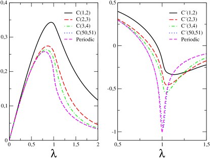
Figure 1: Left hand side: The nearest neighbor concurrence of the open boundary Ising model for different locations relative to the end as function of $\lambda$ for $N=101$. Right hand side: The derivative of the concurrence with respect to $\lambda$.

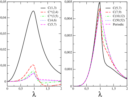
Figure 2: The generalized next-nearest neighbor concurrence of the open boundary Ising model for different locations relative to the end of the chain as function of $\lambda$ for $N=101$.

We first consider the nearest neighbor concurrence of the Ising chain with open boundaries ($\kappa=0$) for a fixed number of sites $N=101$ as parameter of $\lambda$, but for various positions relative to the end of the chain. The results are displayed on the left hand side of Fig. 1. As expected, the concurrence of the periodic model is approached as one moves inside the chain and the difference between ${\cal C}(50,51)$ and ${\cal C}(i,i+1)$ of the periodic system is hardly seen. Nevertheless, the derivative of the concurrence with respect to the coupling parameter $\lambda$, ${\cal C}^{\prime}\equiv d{\cal C}/d\lambda$, still shows appreciable differences for $\lambda\approx 1$ (right hand side of Fig. 1).

We also investigated the scaling behavior of the minimum of ${\cal C}^{\prime}(1,2)$, $\lambda_{min}$, for different systems sizes up to $N=231$. We did not find finite-size scaling behavior for the position of the minimum as is the case for the translationally invariant modelOsterloh et al. (2002). The curve of ${\cal C}^{\prime}(1,2)$, shown on the right hand side of Fig. 1, is thus already close to the curve for $N\to\infty$ with a broad minimum around $\lambda_{min}\approx 1.1$.

The absence of finite-size scaling of the concurrence is also manifested in the case of the next-nearest neighbor concurrence for different system sizes $N$. Whereas for the periodic system the maximum of ${\cal C}(i,i+2)$ decreases monotonically for $N\to\infty$,Osterloh et al. (2002) there is practically no change of ${\cal C}(1,3)$ of the open chain for $N\lower 3.50006pt\hbox{$\stackrel{{\scriptstyle\textstyle>}}{{\sim}}$}51$.

In Fig. 2, the generalized next-nearest neighbor concurrence ${\cal C}^{*}(i,i+2)$ of the open boundary Ising model is shown for different locations relative to the end of the chain as function of $\lambda$ for $N=101$. On the left hand side of Fig. 2, results are shown for sites close to the end of the chain. Notice that the generalized concurrence becomes negative for $i=2,3$ for $\lambda>1$ which is not related to the quantum phase transition. The crossover of the boundary behavior to the bulk behavior is thus discontinuous. On the right hand side of Fig. 2, the next-nearest neighbor concurrence approaches the result of the system with periodic boundary conditions as one moves inside the chain.

II.3.2 Generalized boundary conditions

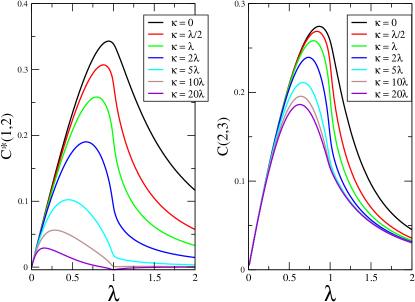
Figure 3: Left hand side: The generalized nearest neighbor concurrence of the closed Ising chain for various coupling strengths $\kappa$ as function of $\lambda$. Left hand side: ${\cal C}^{*}(1,2)$. Right hand side: ${\cal C}(2,3)$.

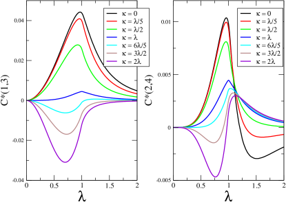
Figure 4: The generalized next-nearest neighbor concurrence of the closed Ising chain for various coupling strengths $\kappa$ as function of $\lambda$. Left hand side: ${\cal C}^{*}(1,3)$. Right hand side: ${\cal C}^{*}(2,4)$.

We now discuss the concurrence for the generalized boundary conditions, introducing the parameter $\kappa$. On the left hand side of Fig. 3, the generalized concurrence of the first two spins ${\cal C}^{*}(1,2)$ is shown as function of $\lambda$ for various coupling strengths $\kappa=0,..,20\lambda$ and $N=101$. For increasing $\kappa>0$, the curves indicate stronger non-analyticity at $\lambda\approx 1$. For $\kappa\lower 3.50006pt\hbox{$\stackrel{{\scriptstyle\textstyle>}}{{\sim}}$}20\lambda$, the generalized concurrence becomes negative around $\lambda=1$ and is ”significantly” positive only in the quantum limit of a strong transverse field ($\lambda<1$). A similar behavior of the concurrence is also found in the case of finite temperatures.Arnesen et al. (2001); Osborne and Nielsen (2002)

On the right hand side of Fig. 3, the concurrence of the second two spins ${\cal C}(2,3)$ is shown. All curves display similar behavior. There is thus a rapid crossover from the boundary to the bulk-regime and the concurrence of periodic boundary conditions is approached for all $\kappa$ as one moves further inside the chain.

To close, we discuss the next-nearest neighbor concurrence ${\cal C}(i,i+2)$ for various values of $\kappa$ and $N=101$. On the left hand side of Fig. 4, the generalized concurrence of the first and the third spin, ${\cal C}^{*}(1,3)$, is shown. For $\kappa\lower 3.50006pt\hbox{$\stackrel{{\scriptstyle\textstyle<}}{{\sim}}$}1$, ${\cal C}^{*}(1,3)$ is positive for all $\lambda$. For $\kappa\lower 3.50006pt\hbox{$\stackrel{{\scriptstyle\textstyle>}}{{\sim}}$}1$, ${\cal C}^{*}(1,3)$ first becomes negative for $\lambda<1$. For $\kappa\lower 3.50006pt\hbox{$\stackrel{{\scriptstyle\textstyle>}}{{\sim}}$}1.5$ ${\cal C}^{*}(1,3)$ is negative for all $\lambda$. On the right hand side of Fig. 4, the generalized concurrence of the second and the forth spin, ${\cal C}^{*}(2,4)$, is shown. For $\kappa\lower 3.50006pt\hbox{$\stackrel{{\scriptstyle\textstyle<}}{{\sim}}$}\lambda/2$, the ${\cal C}^{*}(2,4)$ is negative for $\lambda\lower 3.50006pt\hbox{$\stackrel{{\scriptstyle\textstyle>}}{{\sim}}$}1$. For $\kappa\lower 3.50006pt\hbox{$\stackrel{{\scriptstyle\textstyle>}}{{\sim}}$}3\lambda/2$, the ${\cal C}^{*}(2,4)$ is negative for $\lambda\lower 3.50006pt\hbox{$\stackrel{{\scriptstyle\textstyle<}}{{\sim}}$}1$. Nevertheless, the maximum value is close to $\lambda=1$ for all cases.

We finally note that the third neighbor concurrence remains zero for all $\lambda$ and all $\kappa$.

II.4 Summary

To conclude, we have calculated the entanglement between qubits at the boundary of a spin chain, whose parameters are tuned to be near a quantum critical point. The calculations show a behavior which differs significantly from the that inside the bulk of the chain. Although the spins are part of the critical chain, we find no signs of the scaling behavior which can be found in the bulk. Still, we could identify a boundary regime, basically given by the first site, and a crossover regime of approximately 10 sites till the bulk behavior is reached. We use the same approach as done previously for the bulkOsterloh et al. (2002); Osborne and Nielsen (2002), although it should be noted that the existence of a finite order parameter in the ordered phase will change these results if the calculations were performed in the presence of an infinitesimal applied field.

III Concurrence at a boundary phase transition

In order to observe critical behavior of the concurrence at the boundary, one has to consider a different model than the simple transverse Ising chain. One possibility would be to introduce an isotropic coupling from spin $N$ to spin $1$ which would lead to an interaction term containing four fermionic operators. A simple solution is thus not possible anymore. In the following, we will consider a similar model, but which can easily be mapped onto the spin-boson model.

III.1 The model

The model with isotropic coupling between the two spins at the end is similar to the model introduced by Garst et al. Garst et al. (2003) (see also Ref. Vojta et al. (2002)). It describes two spin-1/2 systems attached to two different electronic reservoirs. They further interact among themselves through an Ising term. We can write the Hamiltonian as

$$H = {H}_{K1}+{H}_{K2}+IS_{z1}S_{z2}\;,$$

$${H}_{Ki} = \sum_{k}\epsilon_{k,\mu}c^{{}^{\dagger}}_{k,\mu,i}c_{k,\mu,i}+J\sum_{k,k^{\prime},\mu,\nu}c_{k,\mu,i}\vec{\sigma}_{\mu,\nu}c_{k^{\prime},\nu,i}\vec{S}_{i}\;.$$

To evaluate the concurrence of the two spins, the $4\times 4$ reduced density matrix in the basis of the eigenstates of $S_{z1}$ and $S_{z2}$ is needed.

The system described by Eq.(LABEL:hamil) undergoes a Kosterlitz-Thouless transition between a phase with a doubly degenerate ground state and a phase with a non degenerate ground state. This transition is equivalent to that in the dissipative two-level systemLeggett et al. (1987); Weiss (1999) as function of the strength of the dissipation. We define the dissipative two-level system as

$${H}_{TLS}=\Delta\sigma_{x}+\sum_{k}|k|b^{{}^{\dagger}}_{k}b_{k}+\lambda\sigma_{z}\sum_{k}\sqrt{k}(b^{{}^{\dagger}}_{k}+b_{k})\;.$$ (19)

The strength of the dissipation can be characterized by a dimensionless parameter, $\alpha\propto\lambda^{2}$, and the model undergoes a transition for $\tilde{\Delta}=\delta/\omega_{c}\ll 1$, where $\omega_{c}$ is the cutoff, and $\alpha=1$. The Kondo model can be mapped onto this model by taking $\Delta\propto\tilde{J_{\perp}}$ and $1-\alpha\propto\tilde{J_{z}}$ Guinea et al. (1985).

To understand the equivalence between these two models, it is best to to consider the limit $I/J\gg 1$ (the transition takes place for all values of this ratio). Let us suppose that $I>0$ so that the Ising coupling is antiferromagnetic. The Hilbert space of the two impurities has four states. The combinations $|\uparrow\uparrow\rangle$ and $|\downarrow\downarrow\rangle$ are almost decoupled from the low energy states, and the transition can be analyzed by considering only the $|\uparrow\downarrow\rangle$ and $|\downarrow\uparrow\rangle$ combinations. Thus, we obtain an effective two state system. The transition is driven by the spin flip processes described by the Kondo terms. These processes involve two simultaneous spin flips in the two reservoirs. Hence, the operator which induces these spin flips leads to the correspondence $\tilde{\Delta}\leftrightarrow J_{\perp}^{2}/(I\omega_{c})$. The scaling dimension of this term, in the Renormalization Group sense, is reduced with respect to the ordinary Kondo Hamiltonian, as two electron-hole pairs must be created. This implies the equivalence $2-\alpha\leftrightarrow\tilde{J_{z}}$. Hence, the transition, which for the ordinary Kondo system takes place when changing the sign of $J_{z}$ now requires a finite value of $J_{z}$.

III.2 Calculation of the concurrence

The $4\times 4$ reduced density matrix can be decomposed into a $2\times 2$ box involving the states $|\uparrow\downarrow\rangle$ and $|\downarrow\uparrow\rangle$, which contains the matrix elements which are affected by the transition, and the remaining elements involving $|\uparrow\uparrow\rangle$ and $|\downarrow\downarrow\rangle$ which are small, and are not modified significantly by the transition. Neglecting these couplings, we find that two of the four eigenvalues of the density matrix are zero. The other two are determined by the matrix

$$\tilde{\rho}\equiv\frac{1}{2}\left(\begin{array}[]{cc}1+\langle\sigma_{z}\rangle&\langle\sigma_{x}\rangle\\ \langle\sigma_{x}\rangle&1-\langle\sigma_{z}\rangle\;.\end{array}\right)$$ (20)

where the operator $\tilde{\sigma}$ is defined using the standard notation of the dissipative two level system, Eq. (19). The entanglement can be written as

$${\cal C}=\sqrt{\langle\sigma_{z}\rangle^{2}+\langle\sigma_{x}\rangle^{2}}\;.$$ (21)

The value of $\langle\sigma_{z}\rangle$ is the order parameter of the transition. The value of $\langle\sigma_{x}\rangle$, at zero temperature, can be calculated from

$$\langle\sigma_{x}\rangle=\frac{\partial E_{0}}{\partial\Delta}\;.$$ (22)

where $E_{0}$ is the energy of the ground state. Using scaling arguments (see appendix B), it can be written as followed:

$$E_{0}=\left\{\begin{array}[]{lr}\frac{C}{1-2\alpha}\left[\Delta\left(\frac{\Delta}{\omega_{c}}\right)^{\frac{\alpha}{1-\alpha}}-\frac{\Delta^{2}}{\omega_{c}}\right]&0<\alpha<\frac{1}{2}\\ 2C\frac{\Delta^{2}}{\omega_{c}}\log\left(\frac{\omega_{c}}{\Delta}\right)&\alpha=\frac{1}{2}\\ \frac{C}{2\alpha-1}\left[\frac{\Delta^{2}}{\omega_{c}}-\Delta\left(\frac{\Delta}{\omega_{c}}\right)^{\frac{\alpha}{1-\alpha}}\right]&\frac{1}{2}<\alpha<1\\ C\left(\frac{\Delta^{2}}{\omega_{c}}-C^{\prime}\omega_{c}e^{-\frac{C^{\prime\prime}\omega_{c}}{\Delta}}\right)&\alpha\sim 1\\ C\frac{\Delta^{2}}{\omega_{c}}&\alpha>1\end{array}\right.$$ (23)

where $C,C^{\prime}$ and $C^{\prime\prime}$ are numerical constants.

If the density matrix is calculated in the absence of a symmetry breaking field, $\langle\sigma_{z}\rangle=0$ even in the ordered phase. Then, from Eq.(21), the concurrence is given by ${\cal C}=|\langle\sigma_{x}\rangle|$, which is completely determined using Eqs. (22) and (23). In the limit $\Delta/\omega_{c}\ll 1$ the interaction with the environment strongly suppresses the entanglement. We expect unusual behavior of the concurrence for $\alpha=1/2$ and $\alpha=1$. The point $\alpha=1/2$ marks the loss of coherent oscillations between the two statesGuinea (1985); not , although the ground state remains non degenerate. Following the analysis in Osterloh et al. (2002), we analyze the behavior of $\partial{\cal C}/\partial\alpha$, as $\alpha$ is the parameter which determines the position of the critical point. The strongest change of this quantity occurs for $\alpha=1/2$, where:

$$\left.\frac{\partial{\cal C}}{\partial\alpha}\right|_{\alpha=1/2}\sim\frac{\Delta}{\omega_{c}}\log\left(\frac{\omega_{c}}{\Delta}\right)$$ (24)

On the other hand, near $\alpha=1$ the value of $\partial{\cal C}/\partial\alpha$ is continuous, as the influence of the critical point has a functional dependence, when $\alpha\rightarrow\alpha_{c}$, of the type $e^{-c/(\alpha_{c}-\alpha)}$. This is the standard behavior at a Kosterlitz-Thouless phase transition. This result suggest that the entanglement is more closely related to the presence of coherence between the two qubits than to the phase transition. The transition takes place well after the coherent oscillations between the $|\uparrow\downarrow\rangle$ and $|\downarrow\uparrow\rangle$ states are completely suppressed. We note though that with a symmetry breaking field, there is a discontinuity of the concurrence at the phase transition Kopp et al. (2007).

IV Von Neumann entropy for dissipative systems

In this section, we will use the von Neumann entropy as measure of entanglement. It is defined for any bipartite system with a ground-state $|\psi\rangle$ by introducing the reduced density matrix with respect to one of the subsystem. For the two subsystems $A$ and $B$, it reads

$$E(\psi)=-\text{Tr}(\rho_{A}\ln\rho_{A})\quad,\quad\rho_{A}=\text{Tr}_{B}(|\psi\rangle\langle\psi|)\;.$$ (25)

In contrast to the concurrence, an analytic expression of the reduced density matrix $\rho_{A}$ does not automatically lead to an analytic expression for the von Neumann entropy. In the following, we show that in the case of integrable dissipative models, the von Neumann entropy can be obtained analytically. We then also discuss the von Neumann entropy of the spin-boson model.

IV.1 Integrable quantum dissipative systems

Modeling the environment by a set of harmonic oscillators Caldeira and Leggett (1983a), the canonical (integrable) model for dissipative systems is described by the following Hamiltonian:

$$H =\frac{p^{2}}{2}+\frac{\omega_{0}^{2}}{2}q^{2}+\sum_{\alpha}\Big{(}\frac{p_{\alpha}^{2}}{2}+\frac{1}{2}\omega_{\alpha}^{2}\big{(}x_{\alpha}-\frac{\lambda_{\alpha}}{\omega_{\alpha}^{2}}q\big{)}^{2}\Big{)}$$ (26)

The operators obey the canonical commutation relations which read ($\hbar=1$)

$$\left[q,p\right]=i\quad,\quad\left[x_{\alpha},p_{\alpha^{\prime}}\right]=i\delta_{\alpha,\alpha^{\prime}}\quad.$$ (27)

The coupling of the system to the bath is completely determined by the spectral function

$$J_{HO}(\omega)=\frac{\pi}{2}\sum_{\alpha}\frac{\lambda_{\alpha}^{2}}{\omega_{\alpha}}\delta(\omega-\omega_{\alpha}).$$ (28)

In the following, we will consider a Ohmic bath with $J_{HO}(\omega)=\eta\omega$ for $\omega\ll\omega_{c}$ and $J_{HO}(\omega)=0$ for $\omega\gg\omega_{c}$, $\omega_{c}$ being the cutoff frequency.

IV.1.1 Caldeira-Leggett model

Let us first consider the free dissipative particle, i.e., we set $\omega_{0}=0$. The model was introduced by Caldeira and Leggett Caldeira and Leggett (1983b) and further investigated by Hakim and Ambegaokar Hakim and Ambegaokar (1985). The latter authors obtained the reduced density matrix via diagonalization of the Hamiltonian. In real space, it reads

$$\langle x|\rho_{A}|x^{\prime}\rangle=e^{-a(x-x^{\prime})^{2}}/L\quad,\quad a=\frac{1}{4}\frac{\eta}{\pi}\ln\left(1+\frac{\omega_{c}^{2}}{\eta^{2}}\right)\;$$ (29)

where $\eta$ denotes the phenomenological friction coefficient and $\omega_{c}$ is the cutoff frequency of the bath, introduced below Eq. (28). Furthermore, $L\to\infty$ denotes the system size and in contrast to the use of Eq. 29 in Ref. Hakim and Ambegaokar (1985), here the normalization is crucial to assure Tr$\rho_{A}=1$.

In order to calculate the entropy of the system, we Taylor expand the logarithm

$$\ln\rho_{A}=-\sum_{n=1}\frac{(1-\rho_{A})^{n}}{n}=-\sum_{n=1}\frac{1}{n}\sum_{k=0}^{n}{n\choose k}(-1)^{k}\rho_{A}^{k}\;.$$ (30)

Further we have

$$\langle x|\rho_{A}^{k}|x^{\prime}\rangle=\sqrt{\frac{\pi}{a}}^{k-1}\sqrt{\frac{1}{k}}e^{-\frac{a}{k}(x-x^{\prime})^{2}}/L^{k}$$ (31)

proved by induction. With the identity

$$\sqrt{\frac{1}{k}}=\frac{1}{\sqrt{\pi}}\int dxe^{-kx^{2}}$$ (32)

we thus obtain for the specific entropy (for general dimension $d$)

$$S=\frac{d}{2}\left[\ln(aL^{2})+\ln(e\pi)\right].$$ (33)

Comparing the above result with the entropy of a particle in a canonical ensemble, we identify $a\sim\lambda^{-2}\propto T$ with $\lambda$ denoting the thermal de Broglie wavelength and $T$ the temperature of the canonical ensemble. Notice that the entropy of a free dissipative particle shows no non-analyticity.

IV.1.2 Dissipative harmonic oscillator

We now include the harmonic potential, i.e., $\omega_{0}\neq 0$. The reduced density matrix of the damped harmonic oscillator is given by Weiss (1999)

$$\langle x|\rho_{A} |x^{\prime}\rangle=\sqrt{\frac{4b}{\pi}}e^{-a(x-x^{\prime})^{2}-b(x+x^{\prime})^{2}}\;,$$ (34)

with $a=\frac{\langle p^{2}\rangle}{2}$ and $b=\frac{1}{8\langle q^{2}\rangle}$. The above expression is deduced such that the correct variance for position and momentum is obtained. At $T=0$ the expectation values are given by

$$\langle q^{2}\rangle =\frac{1}{2\omega_{0}}f(\kappa)\quad,\quad\langle p^{2}\rangle=\omega_{0}^{2}(1-2\kappa^{2})\langle q^{2}\rangle+\frac{2\omega_{0}\kappa}{\pi}\ln\left(\frac{\omega_{c}}{\omega_{0}}\right)\;,$$ (35)

with $\kappa=\eta/2\omega_{0}$ and

$$f(\kappa)=\frac{1}{\pi}\frac{\ln\left[(\kappa+\sqrt{\kappa^{2}-1})/(\kappa-\sqrt{\kappa^{2}-1})\right]}{\sqrt{\kappa^{2}-1}}\quad.$$ (36)

The parameter $\kappa$ represents the friction parameter and the system experiences a crossover from coherent to incoherent oscillations at $\kappa=1$.

Taylor expanding the logarithm of the entropy, Eq. (30), leads to the evaluation of the general $n$-dimensional integral

$$\int_{-\infty}^{\infty}dx_{1}..dx_{n}\exp\left(-\sum_{i,j=1}^{n}x_{i}A_{i,j}x_{j}\right)=\frac{\pi^{n/2}}{\sqrt{\text{det}A}}$$ (37)

where $A$ is given by the translationally invariant tight-binding matrix with $A_{i,i}=2(a+b)$, $A_{i+1,i}=A_{i,i+1}=-(a-b)$ ($n+1\equiv 1$) and zero otherwise. The determinant of the matrix is given by its eigenvalues and reads

$$\text{det}A=(2a)^{n}(1-b/a)^{n}\prod_{m=1}^{n}\left[1+\frac{2b}{a-b}-\cos k_{m}\right]$$ (38)

with $k_{m}=2\pi m/n$.

The determinant can be easily evaluated for large cut-offs $\omega_{c}\rightarrow\infty$ Stauber and Guinea (2006): Considering the $n$-dimensional translationally invariant, but non-Hermitian matrix $\widetilde{A}_{i,i}=1$, $\widetilde{A}_{i+1,i}=1-\varepsilon$ ($n+1\equiv 1$) and zero otherwise, one obtains the following formula:

$$\prod_{m=1}^{n}\left[1+\frac{\varepsilon^{2}}{2(1-\varepsilon)}-\cos k_{m}\right]=\frac{(1-(1-\varepsilon)^{n})^{2}}{2^{n}(1-\varepsilon)^{n}}$$ (39)

For $\omega_{c}/\omega_{0}\gg 1$, we have

$$a/b =4\langle q^{2}\rangle\langle p^{2}\rangle$$

$$=f(\kappa)\left[(1-2\kappa^{2})f(\kappa)+\frac{4\kappa}{\pi}\ln\left(\frac{\omega_{c}}{\omega_{0}}\right)\right]\gg 1.$$ (40)

In this limit, we can thus set $\varepsilon^{2}=4b/a\ll 1$ and the $n$-dimensional integral can be approximated to yield

$$\int dx\langle x|\rho_{A}^{n}|x\rangle \rightarrow\frac{\tilde{\varepsilon}^{n}}{1-(1-\varepsilon)^{n}}\;,$$ (41)

with $\tilde{\varepsilon}\equiv\varepsilon\sqrt{1-\varepsilon}/\sqrt{1-\varepsilon^{2}/4}$. Expanding the denominator as geometrical series, we then have for the entropy

$$S =-\left(\frac{\tilde{\varepsilon}}{\varepsilon}\ln\tilde{\varepsilon}+\frac{\tilde{\varepsilon}}{\varepsilon^{2}}\ln(1-\varepsilon)\right).$$ (42)

In the limit $\varepsilon\approx\tilde{\varepsilon}\ll 1$, the leading behavior of the entropy is given by $S\sim\ln(a/b)$.

The determinant can also be calculated exactly as was done in Ref. Kopp et al. (2007). This yields the exact expression of the von Neumann entropy,

$$S=-\frac{1}{2}\ln\left(\frac{4b}{a-b}\right)-\frac{a}{2b}\ln\left(\frac{\sqrt{a}-\sqrt{b}}{\sqrt{a}+\sqrt{b}}\right)\;.$$ (43)

The von Neumann entropy is plotted in Fig. 5 for various cutoff energies $\omega_{c}$ as function of the coupling constant $\kappa$. Notice that in all curves a crossover behavior occurs at $\kappa\approx 1$, where coherent and incoherent oscillations interchange.

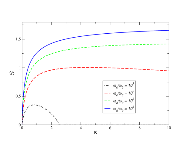
Figure 5: The entropy $S$ of the dissipative oscillator with Ohmic coupling as function of the dimensionless coupling strength $\kappa$ for various cut-off frequencies $\omega_{c}$.

IV.2 Spin-boson model

In section III, the spin-boson model or dissipative two-level system was already introduced and the concurrence was calculated in the context of a two-impurity Kondo model. Here, we want to compute the von-Neumann entropy for this system. Since we will discuss several bath types, the Hamiltonian without bias shall be defined with general coupling constants $\lambda_{k}$ as

$$H=\frac{\Delta_{0}}{2}\sigma_{x}+\sum_{k}\omega_{k}b_{k}^{\dagger}b_{k}+\sigma_{z}\sum_{k}\frac{\lambda_{k}}{2}(b_{k}+b_{k}^{\dagger})\quad.$$ (44)

Again, the operators $b_{k}^{(\dagger)}$ resemble the bath degrees of freedom and $\sigma_{x}$, $\sigma_{y}$, $\sigma_{z}$ denote the Pauli spin matrices. The coupling constants $\lambda_{k}$ give rise to the spectral function

$$J(\omega)=\sum_{k}\lambda_{k}^{2}\delta(\omega-\omega_{k}).$$ (45)

In the relevant low-energy regime, the spectral function is generally parameterized as a power-law, i.e., $J(\omega)\propto 2\alpha\omega^{s}\Lambda_{0}^{1-s}$ where $\alpha$ denotes the coupling constant, $s$ the bath type ($s=1$ defines the previously discussed Ohmic dissipation) and $\Lambda_{0}$ the cutoff-frequency. The change in notation ($\omega_{c}\rightarrow\Lambda_{0}$) will be convenient in the context of the scaling approach.

With $A$ denoting the spin-1/2 system, the reduced density matrix of the spin-boson model is given by

$$\rho_{A}=\frac{1}{2}\begin{pmatrix}1+\langle\sigma_{z}\rangle&\langle\sigma_{x}\rangle\\ \langle\sigma_{x}\rangle&1-\langle\sigma_{z}\rangle\end{pmatrix}.$$ (46)

Since there is no symmetry breaking field in the above Hamiltonian, we set $\langle\sigma_{z}\rangle=0$. The eigenvalues are thus given by $\lambda_{\pm}=(1\pm\langle\sigma_{x}\rangle)/2$ and the entropy reads

$$S=-\frac{1}{2}\left[\ln\left((1-\langle\sigma_{x}\rangle^{2}\right)/4)+\langle\sigma_{x}\rangle\ln\left(\frac{1+\langle\sigma_{x}\rangle}{1-\langle\sigma_{x}\rangle}\right)\right].$$ (47)

The value of $\langle\sigma_{x}\rangle$, at zero temperature, is given by

$$\langle\sigma_{x}\rangle=2\frac{\partial E_{0}}{\partial\Delta_{0}}$$ (48)

where $E_{0}$ is the energy of the ground-state. To obtain the ground-state energy, a scaling analysis for the free energy at arbitrary temperature is considered as before (see appendix B). $E_{0}(\Delta_{0})$ and $\langle\sigma_{x}\rangle$ will then set the basis for our discussion on the entanglement properties of the spin-boson model, see Eq. (47).

IV.2.1 Ohmic dissipation

In the Ohmic case ($s=1$), there is a phase transition at zero temperature at the critical coupling strength $\alpha=1+O(\Delta/\Lambda_{0})$ Bray and Moore (1982); Chakravarty (1982). The transition is also reflected by the renormalized tunnel matrix element $\Delta_{\rm ren}$ which reads $\Delta_{\rm ren}=\Delta_{0}(\Delta_{0}/\Lambda_{0})^{\alpha/(1-\alpha)}$ for $\alpha<1$ and $\Delta_{\rm ren}=0$ for $\alpha>1$.

The von Neumann entropy of the spin-boson model with Ohmic dissipation was first discussed by means of a renormalization group approachCosti and McKenzie (2003) and later also by the thermodynamical Bethe ansatzKopp and Hur (2007). Here, we will obtain the von Neumann entropy within a scaling approach which can also be extended to non-Ohmic dissipation. In this approach, the free energy is given by (see appendix B)

$$F=\int_{\Delta_{\rm ren}}^{\Lambda_{0}}\left(\frac{\Delta(\Lambda)}{\Lambda}\right)^{2}d\Lambda\;.$$ (49)

With $\Delta(\Lambda)=\Delta_{0}(\Lambda/\Lambda_{0})^{\alpha}$, the ground state energy $E_{0}$ is then given by Eq.(23) and the discussion is similar to the one in section III.2. For $\alpha=1/2$, we thus have

$$\frac{d\ln\langle\sigma_{x}\rangle}{d\alpha}\Big{|}_{\alpha=1/2}\propto\ln\left(\frac{\Delta_{0}}{\Lambda_{0}}\right)\;.$$ (50)

In the scaling limit $\Delta_{0}/\Lambda_{0}\rightarrow\infty$, this quantity diverges logarithmically. This is shown on the right hand side of Fig. 6. The entropy $S$ of the dissipative two-level system with Ohmic coupling is plotted in Fig. 6 as function of the dimensionless coupling strength $\alpha$ for various cutoff frequencies $\Lambda_{0}$. The entropy quickly saturates after the transition from coherent to incoherent oscillations at $\alpha=1/2$ as can be seen in terms of $\ln\langle\sigma_{x}\rangle$ on the left hand side of Fig. 6.

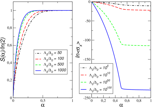
Figure 6: Left hand side: The entropy $S$ of the spin-boson model with Ohmic coupling in units of $\ln(2)$ as function of the dimensionless coupling strength $\alpha$ for various cut-off frequencies $\Lambda_{0}$. The right hand side shows $\ln\langle\sigma_{x}\rangle$ which derivative with respect to the coupling approaches a step-like function in the scaling limit $\Delta_{0}/\Lambda_{0}\rightarrow 0$.

IV.2.2 Non-Ohmic dissipation

The calculation of $E_{0}(\Delta_{0})$ and $\langle\sigma_{x}\rangle$ can be extended to the spin-boson model with non-Ohmic dissipation ($s\neq 1$). In general, the dependence of the effective tunneling term on the cutoff, $\Delta(\Lambda)$, is:

$$\Delta(\Lambda)=\Delta_{0}\exp\left(-\frac{1}{2}\int_{\Lambda}^{\Lambda_{0}}\frac{J(\omega)}{\omega^{2}}d\omega\right)$$ (51)

with the spectral function given in Eq. (45). A renormalized low energy term, $\Delta_{\rm ren}$, can be defined by

$$\Delta_{\rm ren}=\Delta_{0}e^{-\int_{\Delta_{\rm ren}}^{\Lambda_{0}}\frac{J(\omega)}{\omega^{2}}d\omega}\;.$$ (52)

The free energy is again determined by Eq. (49), though cannot be evaluated analytically, anymore. The scaling behavior of the renormalized tunneling given in Eq. (51) is no longer a power law, as in the Ohmic case. Still, we can distinguish two limits:

i) The renormalization of $\Delta(\Lambda)$ is slow. In this case, the integral in Eq. (49) is dominated by the region $\Lambda\sim\Lambda_{0}$, where the function in the integrand goes as $\Lambda^{-2}$. The integral is dominated by its higher cutoff, $\Lambda_{0}$, and the contribution from the region near the lower cutoff, $\Delta_{\rm ren}$, can be neglected. Then, we obtain that $F(\Delta_{0})\sim\Delta_{0}^{2}/\Lambda_{0}$.

ii) The renormalization of $\Delta(\Lambda)$ is fast. In this case, the contribution to the integral in Eq. (49) from the region $\Lambda\approx\Lambda_{0}$ is small. The value of the integral is dominated by the region near $\Lambda\simeq\Delta_{\rm ren}$. As $\Delta_{\rm ren}$ is the only quantity with dimensions of energy needed to describe the properties of the system in this range, we expect that $F(\Delta_{0})\approx\Delta_{\rm ren}$.

In the scaling limit, $\Delta_{0}/\Lambda_{0}\ll 1$, the values of the two terms, $\Delta_{\rm ren}$ and $\Delta_{0}^{2}/\Lambda_{0}$, become very different. In addition, there are no other energy scales which can qualitatively modify the properties of the system. We thus conclude that only the two terms mentioned above will contribute to the free energy. Hence, we can write:

$$F(\Delta_{0})\simeq{\rm max}\left(\Delta_{\rm ren},\frac{\Delta_{0}^{2}}{\Lambda_{0}}\right)$$ (53)

In the following, we will use this conjecture to discuss super- and sub-Ohmic dissipation.

• Super-Ohmic dissipation. In the super-Ohmic case ($s>1$), Eq. (52) always has a solution and, moreover, we can also set the lower limit of the integral to zero. This yields

  $$\Delta_{\rm ren}=\Delta_{0}e^{-\int_{0}^{\Lambda_{0}}\frac{J(\omega)}{\omega^{2}}d\omega}\approx\Delta_{0}e^{-\alpha/(s-1)}.$$ (54)

  For $\alpha\gg 1$ we have $\Delta_{\rm ren}\ll\Delta_{0}$, but there is no transition from localized to delocalized behavior.

  Using Eq. (53) in the super-Ohmic case $s>1$, we can approximately write:

  $$\langle\sigma_{x}\rangle\simeq{\rm max}\left(e^{-\alpha/(s-1)},\frac{\Delta_{0}}{\Lambda_{0}}\right)$$ (55)

  We thus find a transition from underdamped to overdamped oscillations at some critical coupling strength $\alpha\sim(s-1)\log(\Lambda_{0}/\Delta_{0})$.

  It is finally interesting to note that the scaling analysis discussed in Ref. Kosterlitz (1976) is equivalent to the scheme used here.

• Sub-Ohmic dissipation. In the sub-Ohmic case ($s<1$), it is not guaranteed that Eq. (52) has a solution. In general, a solution only exists when $\Delta_{0}/\Lambda_{0}$ is not much smaller than 1.

  The existence of a phase transition in case of a sub-Ohmic bath was first proved in Ref. Spohn and Dümcke (1985). Whereas the relation in Eq. (52) and a similar analysis based on flow equations for Hamiltonians Kehrein and Mielke (1996) yields a discontinuous transition between the localized and delocalized regimes, detailed numerical calculations suggest that the transition is continuous Bulla et al. (2003).

  Since there is a phase transition from localized to non-localized behavior, there might also be a transition between overdamped to underdamped oscillation. In Ref. Stauber and Mielke (2002), this transition was discussed on the basis of spectral functions analogous to the discussion of Refs. Guinea (1985); Costi and Kieffer (1996) for Ohmic dissipation. It was found that for $s>0.5$ the transition takes place for lower values of $\alpha$ as in the Ohmic case, e.g., for $s=0.8$ and $\Lambda_{0}/\Delta_{0}=10$ the transition coupling strength is $\alpha^{*}\approx 0.2$. For a recent discussion on the spectral properties using the Numerical Renormalization Group, see Ref. (Bull and Vojta (2007)).

  Using Eqs. (52) and (53) yields for the sub-Ohmic case the following qualitative behavior:

  $$\langle\sigma_{x}\rangle\simeq\left\{\begin{array}[]{llr}1&{\rm delocalized\,\,\,regime}&\frac{\Delta_{0}}{\Lambda_{0}}\simeq 1\\ \frac{\Delta_{0}}{\Lambda_{0}}&{\rm localized\,\,\,regime}&\frac{\Delta_{0}}{\Lambda_{0}}\ll 1\end{array}\right.$$ (56)

  The analysis used in the previous cases leads us to expect coherent oscillations in the delocalized regime.

  We can extend the study of the sub-Ohmic case to the vicinity of the second order phase transition described in Ref. Vojta et al. (2005), which in our notation takes place for $\alpha=s\Delta_{0}/\Lambda_{0}\ll 1$. In this regime, which cannot be studied using the Franck-Condon like renormalization of Eq. (52), we use the renormalization scheme around the fully coherent state proposed in Ref. Vojta et al. (2005). To one-loop order, the beta-function for the dimensionless quantity (expressed in our notation) $\tilde{\kappa}=(\alpha\Lambda)/\Delta$ then reads

  $$\beta(\tilde{\kappa})=-s\tilde{\kappa}+\tilde{\kappa}^{2}.$$ (57)

  Near the transition, in the delocalized phase, $\tilde{\kappa}$ thus scales towards zero as

  $$\tilde{\kappa}(\Lambda)=\tilde{\kappa}_{0}\left(\frac{\Lambda}{\Lambda_{0}}\right)^{s}\;.$$ (58)

  The scaling of $\langle\sigma_{x}\rangle$ is

  $$\frac{\partial\langle\sigma_{x}\rangle}{\partial\Lambda}=-\tilde{\kappa}(\Lambda)\frac{\Delta}{\Lambda^{2}}\;.$$ (59)

  The fact that the scheme assumes a fully coherent state as a starting point implies that $\Delta$ is not renormalized. Inserting Eq. (58) into Eq. (59), we find:

  $$\frac{\partial\langle\sigma_{x}\rangle}{\partial\Lambda}=-\tilde{\kappa}_{0}\left(\frac{\Lambda}{\Lambda_{0}}\right)^{s}\frac{\Delta_{0}}{\Lambda^{2}}$$ (60)

  

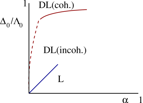
  Figure 7: Schematic picture of the different regimes in the sub-Ohmic dissipative TLS studied in the text. DL stands for the delocalized phase, while L denotes the localized phase. The lower blue line denotes the continuous transition studied in Ref. Vojta et al. (2005). The red line marks the boundaries of a regime characterized by a small renormalization of the tunneling rate, Eq. (52), and coherent oscillations.

  If we calculate $\langle\sigma_{x}\rangle$ from this equation, we find that the resulting integral diverges as $\Lambda\rightarrow 0$ for $s\leq 1$. This result implies that $\langle\sigma_{x}\rangle\ll 1$. For sufficiently low values of the effective cutoff, $\Lambda$, the value of $\langle\sigma_{x}\rangle$ can be calculated using a perturbation expansion on $\Delta_{0}$, leading to $\langle\sigma_{x}\rangle\sim\Delta_{0}/\Lambda_{0}$. This result implies the absence of coherent oscillations. A schematic picture of the regimes studied for the sub-Ohmic TLS is shown in Fig. [7].

We finally note that the entanglement of a spin-1/2 particle coupled to a sub-Ohmic environment has recently been discussed in Ref. Hur et al. (2007).

V Non-local information measure

Quantum measurement is closely connected with the collapse of the wave function and due to the recent advances in quantum engineering, the concept of “information” has to be reconsidered when one deals with quantum mechanical systems. But instead of introducing a new concept of quantum information “from scratch”, one can also start with the measuring process and see what information can be extracted. This line was recently pursued by Zurek and coworkers Ollivier et al. (2005) by proposing that in a classical description, information can be obtained by measuring the environment to which it is coupled. This approach seems even more appropriate for quantum mechanical systems.

V.1 The model and information measure

Figure 8: a) Measuring the system at the left end of the environment. b) Measuring part of the environment. c) Measuring the system and part of the environment simultaneously.

In this section, we want to employ an information measure based on the measurement process and apply it to a dissipative quantum system. The model will consist of a harmonic chain with open boundaries. If the mass of the first (quantum mechanical) particle is large compared to the other masses, one speaks of the Rubin model Rubin (1964), but for simplicity, we will choose all masses equally, here. In subsection V.2, we will then distinguish between the spring constant of the bulk and of the edge. The Hamiltonian is given by

$$H=\sum_{n}\left(\frac{p_{n}^{2}}{2m}+\frac{f}{2}(x_{n+1}-x_{n})^{2}\right)\;.$$ (61)

The particle at the left end of the chain shall denote our system which is coupled to the environment $B_{1}$ (filled and empty circles in Fig. 8a), respectively).

• Measuring the system means that one is only interested in the mean value of the environment. The relevant density matrix is thus obtained by tracing out the bath degrees of freedom. The von Neumann entropy is known to be a good measure to characterize the ground state. We thus have

  $$E_{1}(\psi)=-\text{Tr}(\rho_{1}\ln\rho_{1})\quad,\quad\rho_{1}=\text{Tr}_{B_{1}}(|\psi\rangle\langle\psi|)\quad.$$ (62)

  The above model can be mapped to the dissipative harmonic oscillator with Ohmic coupling. This is done by diagonalizing the bath modes

  $$x_{n}=\sqrt{\frac{2}{\pi}}\int_{0}^{\pi}dk\sin(kn)x(k)$$ (63)

  and results in the following representation of the Hamiltonian:

  $$H=\frac{p^{2}}{2m}+\frac{f}{2}x+\sum_{k}\left(\frac{p_{k}^{2}}{2m}+\frac{m\omega_{k}^{2}}{2}x_{k}^{2}\right)+x\sum_{k}\lambda_{k}x_{k}$$ (64)

• In order to apply the information approach proposed in Ref. Ollivier et al. (2005), we will now pick out one of the environmental particles, see Fig. 8b). Again, the dissipative system (61) can be brought into more familiar form by diagonalizing the left and the right part of the environment separately. This formally results in the problem where a quantum mechanical particle in a harmonic potential is coupled to two baths. But since the left and the right reservoir linearly couple to the same spatial coordinate, they are indistinguishable. The resulting model is thus the standard dissipative harmonic oscillator with modified coupling functions $\lambda_{k}$ as given by Eq. (64).

  The relevant density matrix for the selected particle of the environment is now obtained by tracing out the bath degrees of freedom without the selected particle plus the system itself, labeled as $B_{2}$. For the von Neumann entropy we thus have

  $$E_{2}(\psi)=-\text{Tr}(\rho_{2}\ln\rho_{2})\quad,\quad\rho_{2}=\text{Tr}_{B_{2}}(|\psi\rangle\langle\psi|)\quad.$$ (65)

• The last step is to measure both, the system at the left end of the chain and the selected particle of the bath, see Fig. 8c). Again, we proceed by decoupling the left and right part of the environment separately. We obtain the following representation of the Hamiltonian in Eq. (61):

  $$H =\frac{p_{1}^{2}+p_{2}^{2}}{2m}+\frac{f}{2}(x_{1}^{2}+x_{2}^{2})+\sum_{k,i=1,2}\left(\frac{p_{k,i}^{2}}{2m}+\frac{m\omega_{k,i}^{2}}{2}x_{k,i}^{2}\right)$$

  $$+x_{1}\sum_{k}\lambda_{k,1}x_{k,1}+x_{2}\sum_{k}\left(\kappa_{k,1}x_{k,1}+\kappa_{k,2}x_{k,2}\right)$$ (66)

  In contrary to case b), here there is a distinction between the two resulting non-interacting reservoirs since one bath is coupled to two particles whereas the other bath only couples to the environmental particle. There is no way of preforming a unitary transformation such that the two reservoirs act as one.

  A similar type of problem has been analyzed by Kohler and Sols where two different baths were coupled to the momentum and to the spatial coordinate, respectively Kohler and Sols (2005). Also from the two-channel Kondo model it is known that two baths can significantly alter the system behavior due to the simultaneous measurement process.Potok et al. (2006) We thus expect that effects of quantum frustration are contained in the employed information measure.

  The von Neumann entropy of the subsystem is given by tracing out the degrees of freedom of the remaining bath $B_{3}$

  $$E_{3}(\psi)=-\text{Tr}(\rho_{3}\ln\rho_{3})\quad,\quad\rho_{3}=\text{Tr}_{B_{3}}(|\psi\rangle\langle\psi|)\quad.$$ (67)

The measure of information which is contained by measuring parts of the environment as proposed by Ref. Ollivier et al. (2005) is now given by

$$E(\psi)=E_{3}(\psi)-E_{1}(\psi)-E_{2}(\psi)\;.$$ (68)

In the following, we will set $N_{2}=0$, i.e., we investigate the entanglement between the two ends. In the context of spin-models, the long-distance entanglement was recently considered using as measure of entanglement the concurrence Venuti et al. (2006). On the other hand, it was shown that the above measure based on the von Neumann entropy only captures classical correlations if it is positive Cerf and Adami (1997).

V.2 Entanglement between the two ends

For explicit calculations, we will consider a simplified version of the above model and neglect the reservoir to the right, i.e., we will set $N_{2}=0$ in Fig. 8 b), c). This amounts to the following question: What is the entanglement between the two ends of a harmonic chain as function of the system size $N$.

The chain is confined by the masses at $x_{0}$ and $x_{N}$. The diagonalization of the harmonic chain for finite length $N-1$ yields

$$x_{n}=\frac{1}{\sqrt{N-1}}\sum_{m=1}^{N-1}\sin(k_{m}n)x_{m}\quad,\quad k_{m}=\frac{\pi m}{N}\;.$$ (69)

The eigenvalues are given by $\omega_{m}^{2}=4f_{B}\sin^{2}(k_{m}/2)$. Here, we have introduced an extra spring constant $f_{B}$ for the masses of the bath to contrast it from the spring constant that connects the two masses at the end with the chain, denoted by $f$.

In the following, we will neglect finite size effects and only consider the case where there are two particles at the end. The case of one particle is then simply obtained by neglecting the second particle and the transformed Hamiltonian reads

$$H =\sum_{i=1,2}\frac{p_{i}^{2}}{2}+\frac{f}{2}q_{i}^{2}+\sum_{m}\Big{(}\frac{p_{m}^{2}}{2}+\frac{\omega_{m}^{2}}{2}x_{m}-\sum_{i=1,2}c_{m}^{i}x_{m}q_{i}\Big{)}\;,$$ (70)

with ($N-1\rightarrow N$)

$$c_{m}^{1}=\frac{f_{B}}{\sqrt{N}}\sin(k_{m})\;,\;c_{m}^{2}=(-1)^{m}\frac{f_{B}}{\sqrt{N}}\sin(k_{m})$$ (71)

and $q_{i=1}=x_{0}$ and $q_{i=2}=x_{N}$.

To obtain the von Neumann entropy of the various subsystems listed in a)-c), we first need to compute the reduced density matrix. The reduced density matrix of dissipative systems is commonly represented as a path integral where the bath degrees of freedom have been integrated out Caldeira and Leggett (1983a); Weiss (1999):

$$\langle q^{\prime\prime}|\rho_{A}|q^{\prime}\rangle\propto\int_{q(0)=q^{\prime}}^{q(\beta)=q^{\prime\prime}}{\mathcal{D}}q\exp(-S_{S}^{(E)}[q]-S_{infl}^{(E)}[q])$$ (72)

Here $S_{S}^{(E)}$ denotes the Euclidean action of the system and $S_{infl}^{(E)}$ the influence on the system due to the environment. For one particle coupled on a linear chain with coupling constant $c_{m}$, we have

$$S_{infl}^{(E)}[q]=-\sum_{m}\frac{c_{m}^{2}}{2}\frac{1}{\beta}\sum_{n}\frac{|q_{n}|^{2}}{\nu_{n}^{2}+\omega_{m}^{2}}$$ (73)

with the Fourier transform

$$q(\tau)=\frac{1}{\beta}\sum_{n}q_{n}\exp(i\nu_{n}\tau)\quad,\quad\nu_{n}=2\pi n/\beta\quad.$$ (74)

For two particles coupled to both ends of a linear chain with coupling constants $c_{m}^{(1/2)}$, we have

$$S_{infl}^{(E)}[q]=-\sum_{m}\frac{1}{2}\frac{1}{\beta}\sum_{n}\frac{|c_{m}^{1}q_{n}^{1}+c_{m}^{2}q_{n}^{2}|^{2}}{\nu_{n}^{2}+\omega_{m}^{2}}\quad.$$ (75)

Notice that there is no potential renormalization in our model originating from the harmonic chain.

Since we have already discussed the von Neumann entropy for a dissipative particle in a harmonic potential, we are left with the case of two particle, see Fig. c). With the coupling coefficient of Eq. (71), the effective action $S=S_{S}^{(E)}+S_{infl}^{(E)}$ can be written as $S=S_{1}+S_{2}+S_{int}$ with

$$S_{i} =\sum_{i=1,2}\frac{1}{2}\frac{1}{\beta}\sum_{n}(\nu_{n}^{2}+\omega_{0}^{2}-\omega_{r}^{2}(\nu_{n}))|q_{n}^{i}|^{2}$$ (76)

the effective action of particle $i$ coupled to the dissipative environment and

$$S_{int} =\frac{1}{\beta}\frac{1}{N}\sum_{n}\omega_{I}^{2}(\nu_{n})\text{Re}(q_{n}^{1}q_{n}^{2})$$ (77)

the effective action describing the interaction between the two particles through the environment. In the above equations, we further defined the potential renormalization $\omega_{r}(\nu_{n})$ and the (system-size independent) effective splitting parameter $\omega_{I}(\nu_{n})$ as

$$\omega_{r}^{2}(\nu_{n}) =\frac{1}{N}\sum_{m=1}^{N-1}\frac{f_{B}^{2}\sin^{2}(k_{m})}{\nu_{n}^{2}+4f_{B}\sin^{2}(k_{m}/2)}\quad,$$ (78)

$$\omega_{I}^{2}(\nu_{n}) =-\sum_{m=1}^{N-1}(-1)^{m}\frac{f_{B}^{2}\sin^{2}(k_{m})}{\nu_{n}^{2}+4f_{B}\sin^{2}(k_{m}/2)}\quad.$$ (79)

By a unitary transformation, $q_{n}^{\pm}=(q_{n}^{1}\pm q_{n}^{2})/\sqrt{2}$, the two modes can be decoupled, i.e., $S=S_{+}+S_{-}$:

$$S_{\pm} =\sum_{i=1,2}\frac{1}{2}\frac{1}{\beta}\sum_{n}(\nu_{n}^{2}+\omega_{0}^{2}-\omega_{r}^{2}(\nu_{n})\pm\omega_{I}^{2}(\nu_{n})/N)|q_{n}^{\pm}|^{2}$$ (80)

The physical behavior of dissipative models is determined by the low-frequency modes of the bath. The action can thus be interpreted as the action of two harmonic oscillators with the effective frequencies $\omega_{\pm}=\sqrt{\tilde{\omega}^{2}\pm(\omega_{I}/N)^{2}}$ where $\tilde{\omega}=\sqrt{\omega_{0}^{2}-\omega_{r}^{2}}$. For $\nu_{n}\rightarrow 0$, we further have $\omega_{r}^{2}=\omega_{I}^{2}=f_{B}/2$.

For the chain with equal spring constant $f_{B}=f$, we have $\omega_{0}^{2}=f/2=f_{B}/2$ and thus $\tilde{\omega}=0$, which indicates a phase-transition to a localized state. For $f>f_{B}$, we can use the results of the entropy of an harmonic oscillator. In the expression of the entropy Eq. (43), only the combination $\langle q^{2}\rangle\langle p^{2}\rangle$ enters, such that the only dependence on the system size $N$ is contained in the term

$$\langle q^{2}\rangle\langle p^{2}\rangle\to\frac{\alpha f(\alpha)}{\pi}\ln\frac{\omega_{c}}{\omega_{\pm}}\quad.$$ (81)

Expanding the logarithm, the linear term cancels and we thus have for the information measure for two particles at the end of a harmonic chain with length $N$ the following scaling behavior:

$$I =E(A+B)-E(A)-E(B)\propto\frac{1}{N^{2}}$$ (82)

VI Summary

In this article, we have investigated the entanglement of quantum systems at the boundary. We have first calculated the entanglement between qubits at the boundary of a spin chain, whose parameters are tuned to be near a quantum critical point. The calculations show a behavior which significantly differs from that inside the bulk of the chain. Although the spins are part of the critical chain, we find no signs of the scaling behavior which can be found in the bulk. We use the same approach as done previously for bulk spinsOsterloh et al. (2002); Osborne and Nielsen (2002), although it should be noted that the existence of a finite order parameter in the ordered phase will change these results if the calculations are performed in the presence of an infinitesimal applied field.

We have also considered the entanglement between two Ising-coupled spins connected to a dissipative environment and which undergo a local quantum phase transition. The system which we have studied belongs to the generic class of systems with a Kosterlitz-Thouless transition at zero temperature, like the Kondo model or the dissipative two level system. The most remarkable feature of our results is that the entanglement properties show a pronounced change at the parameter values where the coherent quantum oscillations between the qubits are lost.

In the second part of this article, the entanglement properties of dissipative systems were investigated using the von Neumann entropy. We first discuss two integrable dissipative quantum systems - the free dissipative particle and the dissipative harmonic oscillator - and calculated the von Neumann entropy. In the former case, we found an analogy to the entropy of a canonical ensemble at temperature $T$. The case of the harmonic oscillator is the more interesting one since it exhibits a transition from underdamped to overdamped oscillations. This transition is also manifested in the entropy, but not as strongly as in the case of the spin-boson model. This is probably due to the absence of a quantum phase transition and that the model can be adequately treated by semi-classical methods as done e.g. in the context of the fluctuation-dissipation theorem Weiss (1999).

We also calculated the von Neumann entropy for the spin-boson model on the basis of a scaling approach for the free energy. Only in the Ohmic case, the resulting integral, i.e., the ground-state energy, could be evaluated and we analyzed the behavior at the transition from underdamped to overdamped oscillations. We found that the change of the logarithm of $\langle\sigma_{x}\rangle$ with respect to the coupling strength $\alpha$ is strongly pronounced at the Toulouse point. In the non-Ohmic case, we argued that the crossover between coherent and decoherent oscillation takes place when the value of $\langle\sigma_{x}\rangle$ becomes comparable to the result obtained using a perturbation expansion in the tunneling matrix (as it is the case for Ohmic dissipation). In this framework, we can also discuss the super-Ohmic and sub-Ohmic dissipative two-level system, respectively. We conclude that entanglement properties are closely connected to the transition of coherent to incoherent tunneling.

In the third part of this paper, we have applied an extended measure of quantum information to a simple model, describing a chain of harmonically coupled particles. We argued that this measure can be applied to relate particles of arbitrary distance (or arbitrary regions of the chain) and that it incorporates features of quantum frustration. We calculated explicitly the information measure which relates the two particles at the two ends of the harmonic chain which decays algebraically with the system size.

VII Acknowledgments

Funding from FCT (Portugal) grant PTDC/FIS/64404/2006 and from MEC (Spain) grant FIS2004-06490-C03-01 is acknowledged.

Appendix A Jordan-Wigner and Bogoljubov Transformation

In this appendix, we start the discussion with the slightly more general anisotropic spin-1/2 Heisenberg model in a homogeneous magnetic field, which is given by

$$H=\sum_{i}\left\{J_{x}s_{i}^{x}s_{i+1}^{x}+J_{y}s_{i}^{y}s_{i+1}^{y}+J_{z}s_{i}^{z}s_{i+1}^{z}-hs_{i}^{z}\right\}\;,$$ (83)

where $s_{i}^{\alpha}\to\sigma_{i}^{\alpha}/2$, $\sigma^{\alpha}$ denoting the Pauli matrices with $\alpha=x,y,z$.

Introducing the new operators $a_{i}=s_{i}^{x}+is_{i}^{y}$ (which leads to $s_{i}^{z}=a_{i}^{\dagger}a_{i}-1/2$), one now performs a Jordan-Wigner transformation Jordan and Wigner (1928)

$$c_{i}=\exp\left\{i\pi\sum_{j=1}^{i-1}a_{j}^{\dagger}a_{j}\right\}a_{i}\quad,\quad a_{i}=\exp\left\{-i\pi\sum_{j=1}^{i-1}c_{j}^{\dagger}c_{j}\right\}c_{i}\quad.$$ (84)

With now anti-commuting $c_{i}$-operators $\{c_{i},c_{j}^{\dagger}\}=\delta_{i,j}$, the Hamiltonian can thus be written in Fermion operators as

$$H=\sum_{i}\left\{\frac{J_{x}+J_{y}}{4}(c_{i}^{\dagger}c_{i+1}+h.c.)\frac{J_{x}-J_{y}}{4}(c_{i}^{\dagger}c_{i+1}^{\dagger}+h.c.)+J_{z}(c_{i}^{\dagger}c_{i}-1/2)(c_{i+1}^{\dagger}c_{i+1}-1/2)-h(c_{i}^{\dagger}c_{i}-1/2)\right\}\;.$$ (85)

For the Ising model in a transverse field we set $J_{y}=J_{z}=0$ which yields

$$H=\frac{J_{x}}{4}\sum_{i}\left[c_{i}^{\dagger}c_{i+1}+c_{i}^{\dagger}c_{i+1}^{\dagger}+h.c.\right]-h\sum_{i}c_{i}^{\dagger}c_{i}+Nh/2\;,$$ (86)

where we chose fixed boundary conditions since $a_{N}^{\dagger}a_{1}\neq c_{N}^{\dagger}c_{1}$. For general boundary conditions, i.e., $\kappa\neq 0$ in Eq. (1), we will neglect the boundary term that involves the operator $\exp(i\pi\sum_{i=1}^{N}c_{i}^{\dagger}c_{i})$ in order to preserve the bilinearity of the model, see Ref. Lieb et al., 1961. Using a more general notation for a bilinear Hamiltonian

$$H=\sum_{i,j=1}\left[A_{i,j}c_{i}^{\dagger}c_{j}+\frac{1}{2}\left(B_{i,j}c_{i}^{\dagger}c_{j}^{\dagger}+h.c\right)\right]\;,$$ (87)

the formal diagonalizing of the above Hamiltonian via a Bogoljubov transformation Bogoliubov (1947) leads to

$$H=\sum_{\alpha=1}^{N}\omega_{\alpha}\eta_{\alpha}^{\dagger}\eta_{\alpha}+\frac{1}{2}\left[\sum_{i=1}^{N}A_{i,i}-\sum_{\alpha=1}^{N}\omega_{\alpha}\right]\;,$$ (88)

where $\eta_{\alpha}=\sum_{i}g_{\alpha,i}c_{i}+h_{\alpha,i}c_{i}^{\dagger}$ are the operators in the diagonal basis.

The Bogoljubov transformation, i.e., the determination of the new eigenenergies $\omega_{\alpha}$ as well as the new operators through $g_{\alpha,i}$ and $h_{\alpha,i}$, is equivalent to solving the eigenvalue problem of the matrix $(A-B)(A+B)$. For the Ising model with open boundary condition, this is equivalent to the problem of a one-dimensional chain with an impurity at the first site, i.e., $(A-B)(A+B)\to(J_{x}/4)^{2}H_{TB}$ with

$$H_{TB}=-\sum_{i=1}^{N-1}2\mu(t_{i}^{\dagger}t_{i+1}+h.c.)+\mu^{2}t_{1}^{\dagger}t_{1}+(\mu^{2}+4)\sum_{i=2}^{N}t_{i}^{\dagger}t_{i}$$ (89)

where $\mu=4h/J_{x}$.

We now want to analyze the eigenvectors and eigenenergies of the tight-binding model. For $1<n<N$, the eigenvectors $x_{i}$ and eigenenergies $\tilde{\omega}_{\alpha}^{2}=\omega_{\alpha}^{2}/(J_{x}/4)^{2}$ are given by the following equations:

$$-2\mu x_{n-1}+(\mu^{2}+4-\tilde{\omega}_{\alpha}^{2})x_{n}-2\mu x_{n+1}=0$$ (90)

With the Ansatz $x_{n}\sim e^{ik_{\alpha}n}$, we have for the extended states

$$\tilde{\omega}_{\alpha}^{2}=\mu^{2}+4-4\mu\cos k_{\alpha}\;.$$ (91)

We are interested in the limit $N\to\infty$ where boundary conditions can be disregarded since $k$ will be continuous. For $\mu>0$, we then have $\tilde{\omega}_{max}=2+\mu$, $\tilde{\omega}_{min}=|2-\mu|$.

For $\mu=2$, the continuum starts at zero energy which represents the critical point. For $\mu<2$, there is an additional “bound” state, i.e., $x_{n}\sim e^{-\kappa n}$. For $n>1$, we then have

$$\tilde{\omega}_{b}^{2}=\mu^{2}+4-2\mu(e^{\kappa}+e^{-\kappa})\;,$$ (92)

and for $n=1$, we have $\tilde{\omega}_{b}^{2}=\mu^{2}-2\mu e^{-\kappa}$. This leads to the solution $e^{-\kappa}=\mu/2$ and thus (for $N\to\infty$)

$$\tilde{\omega}_{b}^{2}=0\;.$$ (93)

The restriction $\mu\leq 2$ follows from the condition $\kappa>0$, i.e., a normalizable eigenfunction. The emergence of the bound state can be interpreted as a loss of coherence. Since it is connected to the appearance of a zero energy mode which is inherent to a quantum phase transition, we believe that this view point can be generalized to other quantum phase transitions.

With $\frac{1}{2}\sum_{i}A_{ii}=-hN/2$, we have for the ground-state energy

$$E_{0}=-\frac{1}{2}\sum_{\alpha}\sqrt{J_{x}^{2}/4+h^{2}-hJ_{x}\cos k_{\alpha}}\;.$$ (94)

With the Hellmann-Feynman theorem $\langle m_{z}\rangle=-\frac{1}{N}\partial_{h}E_{0}$, we have for $N\to\infty$

$$\langle m_{z}\rangle=\frac{1}{2\pi}\int_{0}^{\pi}dk\frac{h-\frac{1}{2}J_{x}\cos k}{J_{x}^{2}/4+h^{2}-hJ_{x}\cos k}\;.$$ (95)

At the critical point $h=h_{c}=J/2$, this leads to the logarithmic divergence of $\partial_{h}\langle m_{z}\rangle$.

For finite temperatures, we have

$$F =-kT\left[-\sum_{\alpha}\frac{\omega_{\alpha}}{2}+\sum_{\alpha}\ln(1+e^{-\beta\omega_{\alpha}})\right]\to-kTN\int_{0}^{\pi}dk\ln\left[2\cosh(\beta\omega(k)/2)\right]\;.$$ (96)

With $\langle m_{z}\rangle=-\frac{1}{N}\partial_{h}F$, we have

$$\langle m_{z}\rangle=\frac{1}{2\pi}\int_{0}^{\pi}dk\frac{h-\frac{1}{2}J_{x}\cos k}{J_{x}^{2}/4+h^{2}-hJ_{x}\cos k}\tanh\left[\frac{\beta}{2}\sqrt{J_{x}^{2}/4+h^{2}-hJ_{x}\cos k}\right]\;.$$ (97)

The singularity of $\partial_{h}\langle m_{z}\rangle$ at $h=h_{c}=J/2$ is thus suppressed for $T>0$.

Appendix B Calculation of the free energy of the dissipative TLS

We calculate the free energy of the dissipative two level system following the scaling approach discussed for the Kondo problem in Refs. Anderson et al. (1970); Anderson and Yuval (1971), and formulated in a more general way in Ref. Cardy (1981). For the general long-ranged Ising model, the scaling approach was first applied by Kosterlitz Kosterlitz (1976).

The partition function of the model can be expanded in powers of $\Delta^{2}$ as

$$Z=\sum_{n}\frac{\Delta^{2n}}{2n!}\int_{0}^{\beta}d\tau_{1}\cdots\int_{0}^{\beta}d\tau_{2n}\prod_{ij=1,..,2n}f[(\tau_{i}-\tau_{j})/\tau_{\rm c}]$$ (98)

where $f[(\tau_{i}-\tau_{j})/\tau_{\rm c}]$ denotes the interaction between the kinks located at positions $\tau_{i}$ and $\tau_{j}$. A term in the series is schematically depicted in Fig. [9]. The scaling procedure lowers the short time cutoff of the theory from $\tau_{\rm c}$ to $\tau_{\rm c}-d\tau_{\rm c}$. This process removes from each term in the sum in Eq. (98) details at times shorter than $\tau_{\rm c}-d\tau_{\rm c}$. The rescaling $\tau_{\rm c}\rightarrow\tau_{\rm c}-d\tau_{\rm c}$ implies the change $\Delta\rightarrow\Delta(1+d\tau_{\rm c}/\tau_{\rm c})$. The dependence of $f[(\tau_{i}-\tau_{j})/\tau_{\rm c}]$ leads to another rescaling, which can be included in a global renormalization of $\Delta$ Anderson et al. (1970); Anderson and Yuval (1971); Cardy (1981). In addition, configurations with an instanton-antiinstanton pair at distances between $\tau_{\rm c}$ and $\tau_{\rm c}-d\tau_{\rm c}$ have to be replaced by configurations where this pair is absent, as schematically shown in Fig. [9]. The number of removed pairs is proportional to $d\tau_{\rm c}/\tau_{\rm c}$. The center of the pair can be anywhere in the interval $0\leq\tau\leq\beta$. The final effect is the rescaling:

$$Z\rightarrow Z\left(1+\Delta^{2}\beta d\tau_{\rm c}\right)$$ (99)

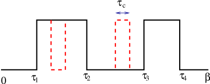
Figure 9: Sketch of the instanton pairs which renormalizes the calculation of the free energy of the dissipative TLS.

Writing $Z$ as $Z=e^{-\beta F}$, where $F$ is the free energy, Eq. (99) can be written as:

$$-\frac{\partial F}{\partial\tau_{\rm c}}=\Delta^{2}(\tau_{\rm c})$$ (100)

In the Ohmic case, the dependence of $\Delta$ on $\tau_{\rm c}=\Lambda^{-1}$ is

$$\Delta(\Lambda)=\Delta_{0}\left(\frac{\Lambda}{\Lambda_{0}}\right)^{\alpha}$$ (101)

and, finally, we find the following relation:

$$\frac{\partial F}{\partial\Lambda}=\left[\frac{\Delta(\Lambda)}{\Lambda}\right]^{2}=\left(\frac{\Delta_{0}}{\Lambda_{0}}\right)^{2}\left(\frac{\Lambda}{\Lambda_{0}}\right)^{2\alpha-2}$$ (102)

This equation ceases to be valid for $\Lambda\simeq\Delta_{\rm ren}$. For finite temperatures, we obtain

$$F(T)=\int_{T}^{\Lambda_{0}}\frac{\partial F}{\partial\Lambda}d\Lambda\;.$$ (103)

It is interesting to apply this analysis to a free two level system. The value of $\Delta_{0}$ does not change under scaling. We find the following expression:

$$\frac{\partial F}{\partial\Lambda}=\left\{\begin{array}[]{lr}\left(\frac{\Delta_{0}}{\Lambda}\right)^{2}&\Delta_{0}\ll\Lambda\\ 0&\Lambda\ll\Delta_{0}\end{array}\right.$$ (104)

Inserting this expression into Eq. (103), we obtain

$$F(T)=\left\{\begin{array}[]{lr}\frac{\Delta_{0}^{2}}{T}&\Delta_{0}\ll T\\ \Delta_{0}&T\ll\Delta_{0}\end{array}\right.$$ (105)

and, finally:

$$\langle\sigma_{x}\rangle=\frac{\partial F}{\partial\Delta_{0}}=\left\{\begin{array}[]{lr}\frac{\Delta_{0}}{T}&\Delta_{0}\ll T\\ 1&T\ll\Delta_{0}\end{array}\right.$$ (106)

in qualitative agreement with the exact result $\langle\sigma_{x}\rangle=\tanh(\Delta_{0}/T)$.

References

- Omnès (1992) R. Omnès, Rev. Mod. Phys. 64, 339 (1992).
- Zurek (2003) W. H. Zurek, Rev. Mod. Phys. 75, 715 (2003).
- Amico et al. (2008) L. Amico, R. Fazio, A. Osterloh, and V. Vedral, Rev. Mod. Phys. 80, 517 (2008).
- Caldeira and Leggett (1983a) A. O. Caldeira and A. J. Leggett, Ann. Phys. (N.Y.) 149, 374 (1983a).
- Feynman and Vernon (1963) R. P. Feynman and F. L. Vernon, Ann. Phys. (N.Y.) 24, 118 (1963).
- Leggett et al. (1987) A. J. Leggett, S. Chakravarty, A. T. Dorsey, M. P. A. Fisher, A. Garg, and W. Zwerger, Rev. Mod. Phys. 51, 1 (1987).
- Weiss (1999) U. Weiss, Quantum dissipative systems (World Scientific, Singapore, 1999).
- Osterloh et al. (2002) A. Osterloh, L. Amico, G. Falci, and R. Fazio, Nature 416, 608 (2002).
- Osborne and Nielsen (2002) T. J. Osborne and M. A. Nielsen, Phys. Rev. A 66, 032110 (2002).
- Vidal et al. (2004) J. Vidal, G. Palacios, and C. Aslangul, Phys. Rev. A 70, 062304 (2004).
- Dusuel and Vidal (2005) S. Dusuel and J. Vidal, Phys. Rev. B 71, 224420 (2005).
- Wootters (1998) W. K. Wootters, Phys. Rev. Lett. 80, 2245 (1998).
- Verstraete et al. (2004a) F. Verstraete, M. Popp, and J. I. Cirac, Phys. Rev. Lett. 92, 027901 (2004a).
- Vidal et al. (2003) G. Vidal, J. I. Latorre, E. Rico, and A. Kitaev, Phys. Rev. Lett. 90, 227902 (2003).
- Verstraete et al. (2004b) F. Verstraete, M. A. Martin-Delgado, and J. I. Cirac, Phys. Rev. Lett. 92, 087201 (2004b).
- Stauber and Guinea (2004) T. Stauber and F. Guinea, Phys. Rev. A 70, 022313 (2004).
- Georges et al. (1996) A. Georges, G. Kotliar, W. Krauth, and M. Rozenberg, Rev. Mod. Phys. 68, 13 (1996).
- Lieb et al. (1961) E. L. Lieb, T. Schultz, and D. Mattis, Ann. Phys. (N. Y.) 16, 407 (1961).
- Pfeuty (1970) P. Pfeuty, Ann. Phys. (N. Y.) 57, 79 (1970).
- Arnesen et al. (2001) M. C. Arnesen, S. Bose, and V. Vedral, Phys. Rev. Lett. 87, 017901 (2001).
- Garst et al. (2003) M. Garst, S. Kehrein, T. Pruschke, A. Rosch, and M. Vojta, Phys. Rev. B 69, 214413 (2003).
- Vojta et al. (2002) M. Vojta, R. Bulla, and W. Hofstteter, Phys. Rev. B 65, 140405 (2002).
- Guinea et al. (1985) F. Guinea, V. Hakim, and A. Muramatsu, Phys. Rev. B 32, 4410 (1985).
- Guinea (1985) F. Guinea, Phys. Rev. B 32, 4486 (1985).
- (25) It is interesting to note that the effective value of for the Ising model considered in the previous section is , as, at criticality, .
- Kopp et al. (2007) A. Kopp, X. Jia, and S. Chakravarty, Ann. Phys. (N. Y.) 322, 1466 (2007).
- Caldeira and Leggett (1983b) A. O. Caldeira and A. J. Leggett, Physica A 121, 587 (1983b).
- Hakim and Ambegaokar (1985) V. Hakim and V. Ambegaokar, Phys. Rev. A 32, 423 (1985).
- Stauber and Guinea (2006) T. Stauber and F. Guinea, Phys. Rev. A 73, 042110 (2006).
- Bray and Moore (1982) A. J. Bray and M. A. Moore, Phys. Rev. Lett. 49, 1545 (1982).
- Chakravarty (1982) S. Chakravarty, Phys. Rev. Lett. 49, 681 (1982).
- Costi and McKenzie (2003) T. A. Costi and R. H. McKenzie, Phys. Rev. B 68, 034301 (2003).
- Kopp and Hur (2007) A. Kopp and K. L. Hur, Phys. Rev. Lett. 98, 220401 (2007).
- Kosterlitz (1976) J. M. Kosterlitz, Phys. Rev. Lett. 37, 1577 (1976).
- Spohn and Dümcke (1985) H. Spohn and R. Dümcke, J. Stat. Phys. 41, 389 (1985).
- Kehrein and Mielke (1996) S. K. Kehrein and A. Mielke, Phys. Lett. A 219, 313 (1996).
- Bulla et al. (2003) R. Bulla, N. H. Tong, and M. Vojta, Phys. Rev. Lett. 91, 170601 (2003).
- Stauber and Mielke (2002) T. Stauber and A. Mielke, Phys. Lett. A 305, 275 (2002).
- Costi and Kieffer (1996) T. A. Costi and C. Kieffer, Phys. Rev. Lett. 76, 1683 (1996).
- Bull and Vojta (2007) F. B. A. R. Bull and M. Vojta, Phys. Rev. Lett. 98, 210402 (2007).
- Vojta et al. (2005) M. Vojta, N. H. Tong, and R. Bulla, Phys. Rev. Lett. 94, 070604 (2005).
- Hur et al. (2007) K. L. Hur, P. Doucet-Beaupré, and W. Hofstetter, Phys. Rev. Lett. 99, 126801 (2007).
- Ollivier et al. (2005) H. Ollivier, D. Poulin, and W. H. Zurek, Phys. Rev. A 72, 042113 (2005).
- Rubin (1964) R. J. Rubin, Phys. Rev. 131, 964 (1964).
- Kohler and Sols (2005) H. Kohler and F. Sols, Phys. Rev. B 72, 180404(R) (2005).
- Potok et al. (2006) R. M. Potok, I. G. Rau, H. Shtrikman, Y. Oreg, and D. Goldhaber-Gordon, Nature 446, 167 (2006).
- Venuti et al. (2006) L. C. Venuti, C. D. E. Boschi, and M. Roncaglia, Phys. Rev. Lett. 96, 247206 (2006).
- Cerf and Adami (1997) N. J. Cerf and C. Adami, Phys. Rev. Lett. 79, 5194 (1997).
- Jordan and Wigner (1928) P. Jordan and E. P. Wigner, Z. Phys. 47, 631 (1928).
- Bogoliubov (1947) N. N. Bogoliubov, J. Phys. Moscow 11, 23 (1947).
- Anderson et al. (1970) P. W. Anderson, G. Yuval, and D. R. Hamann, Phys. Rev. B 1, 4464 (1970).
- Anderson and Yuval (1971) P. W. Anderson and G. Yuval, J. Phys. C: Cond. Mat. 4, 607 (1971).
- Cardy (1981) J. L. Cardy, J. Phys. A: Math. and Gen. 14, 1407 (1981).