Stochastic optimization on continuous domains with finite-time guarantees by Markov chain Monte Carlo methods

Abstract

We introduce bounds on the finite-time performance of Markov chain Monte Carlo algorithms in approaching the global solution of stochastic optimization problems over continuous domains.A comparison with other state-of-the-art methods having finite-time guarantees for solving stochastic programming problems is included.

I Introduction

In principle, any optimization problem on a finite domain can be solved by an exhaustive search. However, this is often beyond computational capacity: the optimization domain of the traveling salesman problem with $100$ cities contains more than $10^{155}$ possible tours [1]. An efficient algorithm to solve the traveling salesman and many similar problems has not yet been found and such problems remain solvable only in principle [2]. Statistical mechanics has inspired widely used methods for finding good approximate solutions in hard discrete optimization problems which defy efficient exact solutions [3, 4, 5, 6]. Here a key idea has been that of simulated annealing [3]: a random search based on the Metropolis-Hastings algorithm, such that the distribution of the elements of the domain visited during the search converges to an equilibrium distribution concentrated around the global optimizers. Convergence and finite-time performance of simulated annealing on finite domains have been evaluated e.g. in [7, 8, 9, 10].

On continuous domains, most popular optimization methods perform a local gradient-based search and in general converge to local optimizers, with the notable exception of convex optimization problems where convergence to the unique global optimizer occurs [11]. Simulated annealing performs a global search and can be easily implemented on continuous domains using the general family of Markov chain Monte Carlo (MCMC) methods [12]. Hence it can be considered a powerful complement to local methods. In this paper, we introduce for the first time rigorous guarantees on the finite-time performance of simulated annealing on continuous domains. We will show that it is possible to derive MCMC algorithms to implement simulated annealing which can find an approximate solution to the problem of optimizing a function of continuous variables, within a specified tolerance and with an arbitrarily high level of confidence after a known finite number of steps. Rigorous guarantees on the finite-time performance of simulated annealing in the optimization of functions of continuous variables have never been obtained before; the only results available state that simulated annealing converges to a global optimizer as the number of steps grows to infinity, e.g. [13, 14, 15, 16, 17], asymptotic convergence rates have been obtained in [18, 19].

The background of our work is twofold. On the one hand, our definition of “approximate domain optimizer”, introduced in Section II as an approximate solution to a global optimization problem, is inspired by the definition of “probably approximate near minimum” introduced by Vidyasagar in [20] for global optimization based on the concept of finite-time learning with known accuracy and confidence of statistical learning theory [21, 22]. In the control field the work of Vidyasagar [20, 22] has been seminal in the development of the so-called randomized approach. Inspired by statistical learning theory, this approach is characterized by the construction of algorithms which make use of independent sampling in order to find probabilistic approximate solutions to difficult control system design applications see e.g. [23, 24, 25] and the references therein. In our work, the definition of approximate domain optimizer will be essential in establishing rigorous guarantees on the finite-time performance of simulated annealing. On the other hand, we show that our rigorous finite-time guarantees can be achieved by the wider class of algorithms based on Markov chain Monte Carlo sampling. Hence, we ground our results on the theory of convergence, with quantitative bounds on the distance to the target distribution, of the Metropolis-Hastings algorithm and MCMC methods [26, 27, 28, 29]. In addition, we demonstrate how, under some quite weak regularity conditions, our definition of approximate domain optimizer can be related to the standard notion of approximate optimization considered in the stochastic programming literature [30, 31, 32, 33]. This link provides theoretical support for the use of simulated annealing and MCMC optimization algorithms, which have been proposed, for example, in [34, 35, 36], for solving stochastic programming problems. In this paper, beyond the presentation of some simple illustrative examples, we will not develop any ready-to-use optimization algorithm. The Metropolis-Hastings algorithm and the general family of MCMC methods have many degrees of freedom. The choice and comparison of specific algorithms goes beyond the scope of the paper.

The paper is organized as follows. In Section II we introduce the definition of approximate domain optimizer and establish a direct relationship between the approximate domain optimizer and the standard notion of approximate optimizer adopted in the stochastic programming literature. In Section III we first recall the reasons why existing results on the convergence of simulated annealing on continuous domain do not provide finite-time guarantees. Then we state the main results of the paper and we discuss their consequences. In Section IV we illustrate the convergence of MCMC algorithms. In Section V we present a simple illustrative numerical example. In Section VI we compare the MCMC approach with other state-of-the-art methods for solving stochastic programming problems with finite-time performance bounds. In Section VII we state our findings and conclude the paper. The Appendix contains all technical proofs. Some of the results of this paper were included in preliminary conference contributions [37, 38].

II Approximate optimizers

Consider an optimization criterion $U:\Theta\rightarrow{\mathbb{R}}$, with $\Theta\subseteq{\mathbb{R}}^{n}$, and let

$$U^{*}:=\sup_{\theta\in\Theta}U(\theta).$$ (1)

The following will be a standing assumption for all our results.

Assumption 1

$\Theta$ has finite Lebesgue measure. $U$ is well defined point-wise, measurable, and bounded between 0 and 1 (i.e. $U(\theta)\in[0,\,1]\,\,\forall\theta\in\Theta$).

In general, any bounded criterion can be scaled to take values in $[0,\,1]$. Given, for example, $U^{\prime}(\theta)\in[\underline{U},\,\overline{U}]$ we can consider the optimization of the modified function

$$U(\theta)=\frac{U^{\prime}(\theta)-\underline{U}}{\overline{U}-\underline{U}}\,,$$

which takes values in $[0,1]$ for all $\theta\in\Theta$. (In this case, we need to multiply the value imprecision, $\epsilon$ below, by $(\overline{U}-\underline{U})$ to obtain its corresponding value in the scale of the original criterion $U^{\prime}$.)

For some results another assumption will be needed.

Assumption 2

$\Theta$ is compact. $U$ is Lipschitz continuous.

We use $L$ to denote the Lipschitz constant of $U$, i.e. $\forall\theta_{1},\theta_{2}\in\Theta,\;|U(\theta_{1})-U(\theta_{2})|\leq L\|\theta_{1}-\theta_{2}\|$. Assumption 2 implies the existence of a global optimizer, i.e. under Assumption 2, we have $\Theta^{*}:=\{\theta\in\Theta\;|\;U(\theta)=U^{*}\}\neq\emptyset.$

If, given an element $\theta$ in $\Theta$, the value $U(\theta)$ can be computed directly, we say that $U$ is a deterministic criterion. In this case the optimization problem (1) is a standard, in general non-linear, non-smooth, programming problem. Examples of such a deterministic optimization criterion are, among many possible others, the design criterion in a robust control design problem [20] and the energy landscape in protein structure prediction [39]. In problems involving random variables, the value $U(\theta)$ can be the expected value of some function $g:\Theta\times X\rightarrow{\mathbb{R}}$ which depends on both the optimization variable $\theta$, and on some random variable $\bm{x}$ with probability distribution $P_{\bm{x}}(\cdot;\theta)$ which may itself depend on $\theta$, i.e.

$$U(\theta)=\int g(x,\theta)P_{\bm{x}}(dx;\theta)\,.$$ (2)

In such problems it is usually not possible to compute $U(\theta)$ directly. In stochastic optimization [30, 31, 32, 40, 34, 35, 36], it is typically assumed that one can obtain independent samples of $\bm{x}$ for a given $\theta$, hence obtain sample values of $g(\bm{x},\theta)$, and thus construct a Monte Carlo estimate of $U(\theta)$. In some application it might not be possible or efficient to obtain independent samples of $\bm{x}$. In this case one has to resort to other Monte Carlo strategies to approximate $U(\theta)$ such as, for example, importance sampling [12]. The Bayesian experimental design of clinical trials is an important application area where expected-value criteria arise [41]. We investigate the optimization of expected-value criteria motivated by problems of aircraft routing [42] and parameter identification for genetic networks [43]. In the particular case that $P_{\bm{x}}(dx;\theta)$ does not depend on $\theta$, the ‘$\inf$’ counterpart of problem (1) is called “empirical risk minimization”, and is studied extensively in statistical learning theory [21, 22]. Conditions on $g$ and $P_{\bm{x}}$ to ensure that $U$ is Lipschitz continuous (for Assumption 2) can be found in [31, pag. 189-190]. The results reported here apply in the same way to the optimization of both deterministic and expected-value criteria.

We introduce two different definitions of approximate solution to the optimization problem (1). The first is the definition of approximate domain optimizer. It will be essential in establishing finite-time guarantees on the performance of MCMC methods.

Definition 1

Let $\epsilon\geq 0$ and $\alpha\in[0,\,1]$ be given numbers. Then $\theta$ is an approximate domain optimizer of $U$ with value imprecision $\epsilon$ and residual domain $\alpha$ if

$$\lambda(\{\theta^{\prime}\in\Theta:U(\theta^{\prime})>U(\theta)+\epsilon\})\leq\alpha\,\lambda(\Theta)$$ (3)

where $\lambda$ denotes the Lebesgue measure.

That is, the function $U$ takes values strictly greater than $U(\theta)+\epsilon$ only on a subset of values of $\theta$ no larger than an $\alpha$ portion of the optimization domain. The smaller $\epsilon$ and $\alpha$ are, the better is the approximation of a true global optimizer. If both $\alpha$ and $\epsilon$ are equal to zero then $U(\theta)$ coincides with the essential supremum of $U$ [44]. We will use

$$\Theta(\epsilon,\alpha):=\{\theta\in\Theta\;|\;\lambda(\{\theta^{\prime}\in\Theta\;|\;U(\theta^{\prime})>U(\theta)+\epsilon\})\leq\alpha\lambda(\Theta)\}$$

to denote the set of approximate domain optimizers with value imprecision $\epsilon$ and residual domain $\alpha$. The intuition that our notion of approximate domain optimizer can be used to obtain formal guarantees on the finite-time performance of optimization methods based on a stochastic search of the domain is already apparent in the work of Vidyasagar. Vidyasagar [22, 20] introduces the similar definition of “probably approximate near minimum” and obtains rigorous finite-time guarantees in the optimization of expected value criteria based on uniform independent sampling of the domain. The method of Vidyasagar has had considerable success in solving difficult control system design applications [20, 23]. Its appeal stems from its rigorous finite-time guarantees which exist without the need for any particular assumption on the optimization criterion.

The following is a more common notion of approximate optimizer.

Definition 2

Let $\epsilon\geq 0$ be a given number. Then $\theta$ is an an approximate value optimizer of $U$ with imprecision $\epsilon$ if $U(\theta^{\prime})\leq U(\theta)+\epsilon$ for all $\theta^{\prime}\in\Theta$.

This notion is commonly used in the stochastic programming literature [30, 31, 32, 40] and provides a direct bound on $U^{*}$: $\theta\in\Theta$ is an approximate value optimizer with imprecision $\epsilon>0$ if and only if $U^{*}\leq U(\theta)+\epsilon$. We will use

$$\Theta^{*}(\epsilon):=\{\theta\in\Theta\;|\;\forall\theta^{\prime}\in\Theta,\;U(\theta^{\prime})\leq U(\theta)+\epsilon\}$$

to denote the set of approximate value optimizers with imprecision $\epsilon$.

It is easy to see that for all $\epsilon$ if $\Theta^{*}\neq\emptyset$ then $\Theta^{*}\subseteq\Theta^{*}(\epsilon)$. Notice that $\Theta^{*}(\epsilon)$ does not coincide with $\Theta(\epsilon,\alpha)$. In fact one can see that approximate value optimality is a stronger concept than approximate domain optimality, in the following sense. For all $\epsilon$ and all $\alpha$, if $\Theta^{*}(\epsilon)\neq\emptyset$ then $\Theta^{*}(\epsilon)\subseteq\Theta(\epsilon,\alpha)$. Conversely, given an approximate domain optimizer it is in general not possible to draw any conclusions about the approximate value optimizers. For example, for any $\alpha$ the function $U:[0,1]\rightarrow[0,1]$ with

$$U(\theta)=\left\{\begin{array}[]{ll}1&\mbox{ if }\theta\in[0,\alpha)\\ 0&\mbox{ if }\theta\in[\alpha,1]\end{array}\right.$$

has the property that $\Theta(\epsilon,\alpha)=\Theta$ for all $\epsilon>0$. Therefore, given $\theta\in\Theta(\epsilon,\alpha)$ it is impossible to draw any conclusions about $U^{*}$; the only possible bound is $U^{*}\leq U(\theta)+1$ which, given that $U(\theta)\in[0,1]$, is meaningless. A relation between domain and value approximate optimality can, however, be established under Assumption 2.

Theorem 1

Let Assumption 2 hold. Let $\theta$ be an approximate domain optimizer with value imprecision $\epsilon$ and residual domain $\alpha$. Then, $\theta$ is also an approximate value optimizer with imprecision

$$\epsilon+\frac{L}{\sqrt{\pi}}\left[\frac{n}{2}\Gamma\left(\frac{n}{2}\right)\right]^{\frac{1}{n}}[\alpha\lambda(\Theta)]^{\frac{1}{n}}$$

where $\Gamma$ denotes the gamma function.

Theorem 1 shows that

$$\theta\in\Theta(\epsilon,\alpha)\Rightarrow U^{*}\leq U(\theta)+\epsilon+\frac{L}{\sqrt{\pi}}\left[\frac{n}{2}\Gamma\left(\frac{n}{2}\right)\right]^{\frac{1}{n}}[\alpha\lambda(\Theta)]^{\frac{1}{n}}\ .$$ (4)

The result allows us to select the value of $\alpha$ in such a way that an approximate domain optimizer with value imprecision $\epsilon$ and residual domain $\alpha$ is also an approximate value optimizer with imprecision $2\epsilon$. To do this, we need to select $\alpha$ so that $\frac{L}{\sqrt{\pi}}\left[\frac{n}{2}\Gamma\left(\frac{n}{2}\right)\right]^{\frac{1}{n}}[\alpha\lambda(\Theta)]^{\frac{1}{n}}\leq\epsilon$ hence

$$\alpha\leq\frac{\left[\frac{\epsilon\sqrt{\pi}}{L}\right]^{n}}{\lambda(\Theta)\left[\frac{n}{2}\Gamma\left(\frac{n}{2}\right)\right]}\,.$$ (5)

To illustrate the above inequality consider the case where the domain $\Theta$ is contained in an $n$-dimensional ball of radius $R$. Notice that under Assumption 2 the existence of such an $R$ is guaranteed. In this case $\lambda(\Theta)=\frac{2\pi^{\frac{n}{2}}}{n\Gamma(\frac{n}{2})}R^{n}\,.$ Therefore (5) becomes

$$\alpha\leq\left(\frac{1}{L}\frac{\epsilon}{R}\right)^{n}\ .$$ (6)

Note that, as $n$ increases, $\alpha$ has to decrease to zero rapidly to ensure the required imprecision of the approximate value optimizer. In this case, $\alpha$ needs to decrease to zero as $\epsilon^{n}$.

III Optimization with MCMC: finite time guarantees

In simulated annealing, a random search based on the Metropolis-Hastings algorithm is carried out, such that the distribution of the elements of the domain visited during the search converges to an equilibrium distribution concentrated around the global optimizers.

Here we adopt equilibrium distributions defined by densities proportional to $[U(\theta)+\delta]^{J}$, where $J$ and $\delta$ are strictly positive parameters. We use

$$\pi(d\theta;J,\delta)\propto[U(\theta)+\delta]^{J}\lambda(d\theta)$$ (7)

to denote this equilibrium distribution. The presence of $\delta$ is a technical condition required in the proof of our main result and will be discussed later on in this section. In our setting, the so-called ‘zero-temperature’ distribution is the limiting distribution $\pi(\,\cdot\,\,;J,\delta)$ for $J\rightarrow\infty$ denoted by $\pi_{\infty}$. It can be shown that under some technical conditions, $\pi_{\infty}$ is a uniform distribution on the set $\Theta^{*}$ of the global maximizers of $U$ [45].

In Fig. 1, we illustrate two algorithms which implement Markov transition kernels with equilibrium distributions $\pi(\,\cdot\,\,;J,\delta)$. Algorithm I is the ‘classical’ Metropolis-Hastings algorithm for the case in which $U$ is a deterministic criterion. Algorithm II is a suitably modified version of the Metropolis-Hastings algorithm for the case in which $U$ is an expected-value criterion in the form of (2). This latter algorithm was devised by Müller [34, 36] and Doucet et al. [35].

Figure 1: The basic iterations of the Metropolis-Hastings algorithm with equilibrium distributions $\pi(\cdot;J,\delta)$ for the maximization of deterministic and expected-value criteria. In both algorithms, $q_{\tilde{\bm{\theta}}}(\cdot|\bm{\theta}_{k})$ is the density of the ‘proposal distribution’.

In the simulated annealing scheme, one would simulate an inhomogeneous chain in which the Markov transition kernel at the $k$-th step of the chain has equilibrium distribution $\pi(\,\cdot\,\,;J_{k},\delta)$ where $\{J_{k}\}_{k=1,2,\dots}$ is a suitably chosen ‘cooling schedule’, i.e. a non-decreasing sequence of values for the exponent $J$. The rationale of simulated annealing is as follows: if the temperature is kept constant, say $J_{k}=J$, then the distribution of the state of the chain, say $P_{\bm{\theta}_{k}}$, tends to the equilibrium distribution $\pi(\,\cdot\,\,;J,\delta)$; if $J\rightarrow\infty$ then the equilibrium distribution $\pi(\,\cdot\,\,;J,\delta)$ tends to the zero-temperature distribution $\pi_{\infty}$; as a result, if the cooling schedule $J_{k}$ tends to $\infty$, one obtains that the distribution of the state of the chain $P_{\bm{\theta}_{k}}$ tends to $\pi_{\infty}$ [13, 14, 15, 16, 17].

The difficulty which must be overcome in order to obtain finite step results on simulated annealing algorithms on a continuous domain is that usually, in an optimization problem defined over continuous variables, the set of global optimizers $\Theta^{*}$ has zero Lebesgue measure (e.g. a set of isolated points). Notice that this is not the case for a finite domain, where the set of global optimizers is of non-null measure with respect to the reference counting measure [7, 8, 9, 10]. It is instructive to look at the issue in terms of the rate of convergence to the target zero-temperature distribution. On a continuous domain, the standard distance between two distributions, say $\mu_{1}$ and $\mu_{2}$, is the total variation distance $\|\mu_{1}-\mu_{2}\|_{\mbox{\tiny TV}}=\sup_{A\in\mathfrak{B}(\Theta)}|\mu_{1}(A)-\mu_{2}(A)|$. If the set of global optimizers $\Theta^{*}$ has zero Lebesgue measure, then the target zero-temperature distribution $\pi_{\infty}$ ends up being a mixture of probability masses on $\Theta^{*}$. On the other hand, the distribution of the state of the chain $P_{\bm{\theta}_{k}}$ is absolutely continuous with respect to the Lebesgue measure (i.e. $\lambda(A)=0\Rightarrow P_{\bm{\theta}_{k}}(A)=0$) by construction for any finite $k$. Hence, if $\Theta^{*}$ has zero Lebesgue measure then it has zero measure also according to $P_{\bm{\theta}_{k}}$. The set $\Theta^{*}$ has however measure 1 according to $\pi_{\infty}$. The distance $\|P_{\bm{\theta}_{k}}-\pi_{\infty}\|_{\mbox{\tiny TV}}$ is then constantly $1$. In general, on a continuous domain, although the distribution of the state of the chain $P_{\bm{\theta}_{k}}$ converges asymptotically to $\pi_{\infty}$, it is not possible to introduce a sensible distance between $P_{\bm{\theta}_{k}}$ and $\pi_{\infty}$ and a rate of convergence to the target distribution cannot even be defined (weak convergence), see [13, Theorem 3.3].

Weak convergence to $\pi_{\infty}$ implies that, asymptotically, $\bm{\theta}_{k}$ eventually hits the set of approximate value optimizers $\Theta^{*}(\epsilon)$, for any $\epsilon>0$, with probability one [13, 14, 15, 16, 17]. In more recent works, bounds on the expected number of iterations before hitting $\Theta^{*}(\epsilon)$ [18] or on $P_{\bm{\theta}_{k}}(\Theta^{*}(\epsilon))$ [19] have been obtained. In [19], a short review of existing bounds is proposed, and under some technical conditions, it is proven that for any $\epsilon>0$ there is a number $C_{\epsilon}$ such that $P_{\bm{\theta}_{k}}(\{\theta\in\Theta\;|\;U(\theta)\leq U^{*}-\epsilon\})\leq C_{\epsilon}k^{-\frac{1}{3}}(1+\log k)$. In general, the expressions in these bounds cannot be computed. For example, in the bound reported here, $C_{\epsilon}$ is not known in advance. Hence, existing bounds can be used to asses the asymptotic rate of convergence but not as stopping criteria.

Here we show that finite-time guarantees for stochastic optimization by MCMC methods on continuous domains can be obtained by selecting a distribution $\pi(\,\cdot\,\,;J,\delta)$ with a finite $J$ as the target distribution in place of the zero-temperature distribution $\pi_{\infty}$. Our definition of approximate domain optimizer given in Section II is essential for establishing this result. The definition of approximate domain optimizers carries an important property, which holds regardless of what the criterion $U$ is: if $\epsilon$ and $\alpha$ have non-zero values then the set of approximate global optimizers $\Theta(\epsilon,\alpha)$ always has non-zero Lebesgue measure. The following theorem establishes a lower bound on the measure of the set $\Theta(\epsilon,\alpha)$ with respect to a distribution $\pi(\cdot;J,\delta)$ with finite $J$. It is important to stress that the result holds universally for any optimization criterion $U$ on a bounded domain. The only minor requirement is that $U$ takes values in $[0,\,1]$.

Theorem 2

Let Assumption 1 hold. Let $\Theta(\epsilon,\alpha)$ be the set of approximate domain optimizers of $U$ with value imprecision $\epsilon$ and residual domain $\alpha$. Let $J\geq 1$ and $\delta>0$, and consider the distribution $\pi(d\theta;J,\delta)\propto[U(\theta)+\delta]^{J}\lambda(d\theta)$. Then, for any $\alpha\in(0,\,1]$ and $\epsilon\in[0,\,1]$, the following inequality holds

$$\pi(\Theta(\epsilon,\alpha);J,\delta)\geq\frac{1}{\mbox{$\displaystyle 1+\left[\frac{1+\delta}{\epsilon+1+\delta}\right]^{\,J}\left[\frac{1}{\alpha}\frac{1+\delta}{\epsilon+\delta}-1\right]\frac{1+\delta}{\delta}$}}\,\,.$$ (8)

Notice that, for given non-zero values of $\epsilon$, $\alpha$, and $\delta$ the right-hand side of (8) can be made arbitrarily close to 1 by choice of $J$. To obtain some insight on this choice it is instructive to turn the bound of Theorem 2 around to provide a lower bound on $J$ which ensures that $\pi(\Theta(\epsilon,\alpha);J,\delta)$ attains some desired value $\sigma$.

Corollary 3

Let the notation and assumptions of Theorem 2 hold. For any $\alpha\in(0,\,1]$, $\epsilon\in(0,\,1]$ and $\sigma\in(0,\,1)$, if

$$J\geq\frac{1+\epsilon+\delta}{\epsilon}\left[\log\frac{\sigma}{1-\sigma}+\log\frac{1}{\alpha}+2\log\frac{1+\delta}{\delta}\right]$$ (9)

then $\pi(\Theta(\epsilon,\alpha);J,\delta)\geq\sigma$.

The importance of the choice of a target distribution $\pi(\,\cdot\,\,;J,\delta)$ with a finite $J$ is that the distance $\|P_{\bm{\theta}_{k}}-\pi(\,\cdot\,\,;J,\delta)\|_{\mbox{\tiny TV}}$ is a meaningful quantity. Convergence of the Metropolis-Hastings algorithm and MCMC methods in total variation distance is a well studied problem. The theory provides simple conditions under which one derives upper bounds on $\|P_{\bm{\theta}_{k}}-\pi(\,\cdot\,\,;J,\delta)\|_{\mbox{\tiny TV}}$ that decrease to zero as $k\rightarrow\infty$ [26, 27, 28, 29]. It is then appropriate to introduce the following finite-time result.

Proposition 4

Let the notation and assumptions of Theorem 2 hold. Assume that $J$ respects the bound of Corollary 3 for given $\alpha$, $\epsilon$, $\delta$ and $\sigma$. Let $\bm{\theta}_{k}$ with distribution $P_{\bm{\theta}_{k}}$ be the state of the chain of an MCMC algorithm with target distribution $\pi(\,\cdot\,\,;J,\delta)$. Then,

$$P_{\bm{\theta}_{k}}(\Theta(\epsilon,\alpha);J,\delta)\geq\sigma-\|P_{\bm{\theta}_{k}}-\pi(\,\cdot\,\,;J,\delta)\|_{\mbox{\tiny TV}}\,.$$

In other words, the statement “$\bm{\theta}_{k}$ is an approximate domain optimizer of $U$ with value imprecision $\epsilon$ and residual domain $\alpha$” can be made with confidence $\sigma-\|P_{\bm{\theta}_{k}}-\pi(\,\cdot\,\,;J,\delta)\|_{\mbox{\tiny TV}}$.

The proof follows directly from the definition of the total variation distance.

If the optimization criterion is Lipschitz continuous, Theorem 2 can be used together with Theorem 1 to derive a lower bound on the measure of the set of approximate value optimizers with a given imprecision with respect to a distribution $\pi(\,\cdot\,\,;J,\delta)$. An example of such a bound is the following.

Proposition 5

Let the notation and assumptions of Theorems 1 and 2 hold. In addition, assume that $\Theta$ is contained in an $n$-dimensional ball of radius $R$. Let $\bm{\theta}_{k}$ with distribution $P_{\bm{\theta}_{k}}$ be the state of the chain of an MCMC algorithm with target distribution $\pi(\,\cdot\,\,;J,\delta)$. For given $\epsilon\in(0,\,1]$ and $\sigma\in(0,\,1)$, if

$$J\geq\frac{1+\epsilon+\delta}{\epsilon}\left[\log\frac{\sigma}{1-\sigma}+n\log\left(\frac{LR}{\epsilon}\right)+2\log\frac{1+\delta}{\delta}\right]$$ (10)

then

$$P_{\bm{\theta}_{k}}(\Theta^{*}(2\epsilon);J,\delta)\geq\sigma-\|P_{\bm{\theta}_{k}}-\pi(\,\cdot\,\,;J,\delta)\|_{\mbox{\tiny TV}}\,.$$

In other words, the statement “$\bm{\theta}_{k}$ is an approximate value optimizer of $U$ with value imprecision $2\epsilon$” can be made with confidence $\sigma-\|P_{\bm{\theta}_{k}}-\pi(\,\cdot\,\,;J,\delta)\|_{\mbox{\tiny TV}}$.

The proof follows by substituting $\alpha$ with the right-hand side of (6) in (9) and from the definition of the total variation distance.

Finally, Theorem 2 provides a criterion for selecting the parameter $\delta$ in $\pi(\,\cdot\,\,;J,\delta)$. For given $\epsilon$ and $\alpha$, there exists an optimal choice of $\delta$ which minimizes the value of $J$ required to ensure $\pi(\Theta(\epsilon,\alpha);J,\delta)\geq\sigma$. The advantage of choosing the smallest $J$, consistent with the required $\sigma$, is computational. The exponent $J$ coincides with the number of Monte Carlo simulations of random variable $\bm{x}$ which must be done at each step in Algorithm II. The smallest $J$ reduces also the peakedness of $\pi(\cdot;J,\delta)$. The higher the peakedness of $\pi(\cdot;J,\delta)$ is the harder is to design a proposal distribution which operates efficiently. In turn, reducing the peakedness of $\pi(\cdot;J,\delta)$ will decrease the number of steps required to achieve the desired reduction of $\|P_{\bm{\theta}_{k}}-\pi(\,\cdot\,\,;J,\delta)\|_{\mbox{\tiny TV}}$.

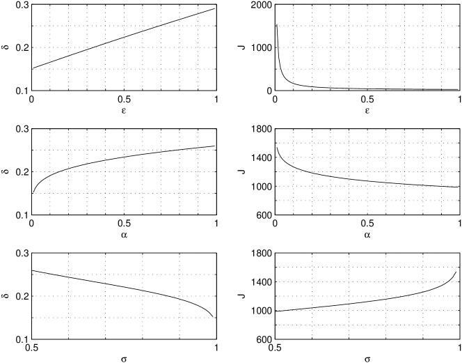
Figure 2: Variation of the optimal $\delta$ and of the corresponding $J$ with respect to $\epsilon$, $\alpha$ and $\sigma$. Two of the three parameters are kept constant for each figure, set to $\epsilon=0.01$, $\alpha=0.01$ and $\sigma=0.99$.

The optimal choice of $\delta$ is specified by the following result.

Proposition 6

For fixed $\epsilon>0$, $\alpha>0$, and $\sigma\in(0.5,\,1)$, the function

$$f(\delta)=\frac{1+\epsilon+\delta}{\epsilon}\left[\log\frac{\sigma}{1-\sigma}+\log\frac{1}{\alpha}+2\log\frac{1+\delta}{\delta}\right]\,,$$

i.e. the right hand side of inequality (9), is convex in $\delta$ and attains its global minimum at the unique solution (for $\delta$) of the equation

$$\log\frac{1+\delta}{\delta}+\log\frac{\sqrt{\sigma}}{\sqrt{1-\sigma}}+\log\frac{1}{\sqrt{\alpha}}=\frac{1+\epsilon+\delta}{\delta(1+\delta)}.$$

For example, if $\epsilon=0.01$, $\alpha=0.01$ and $\sigma=0.99$, then one obtains $\delta=0.15$ and $J=1540$. Plots of the value of the optimal $\delta$ and of the corresponding value of $J$ for different values of $\epsilon$, $\alpha$ and $\sigma$ are shown in Fig. 2. Notice that the result of Proposition 6 holds also for inequality (10) provided that $\alpha$ in the statement of Proposition 6 is replaced by the right hand side of (6).

IV Convergence

In this section we illustrate the statement of Proposition 4. We base the discussion on the simplest available result on the convergence of MCMC methods in total variation distance, taken from [28]. In this case, the proposal distribution, denoted by its density $q_{\tilde{\bm{\theta}}}(\theta|\bm{\theta}_{k})$ in Algorithms I and II, is independent of the current state $\bm{\theta}_{k}$.

Theorem 7 ([28])

Let $P_{\bm{\theta}_{k}}$ be the distribution of the state of the chain in the Metropolis-Hastings algorithm with an independent proposal distribution. Let $\pi$ denote the target distribution. Let $p$ and $q$ denote respectively the density of $\pi$ and the density of the proposal distribution and assume that $p(\theta)>0,\,\forall\theta\in\Theta$ and $q(\theta)>0,\,\forall\theta\in\Theta$. If there exists $M$ such that $p(\theta)\leq Mq(\theta)\,,\,\,\,\forall\theta\in\Theta$, then

$$\left\|\pi-P_{\bm{\theta}_{k}}\right\|_{\mbox{\tiny TV}}\leq\left(1-\frac{1}{M}\right)^{k}.$$ (11)

Proof: See [28, Theorem 2.1], or [12, Theorem 7.8].
Here, we chose $q_{\tilde{\bm{\theta}}}$ as the uniform distribution over $\Theta$. Sampling using an independent uniform proposal distribution is a naïve strategy in an MCMC approach and cannot be expected to perform efficiently [12]. However, it allows us to present some simple illustrative examples where convergence bounds can be derived with a few basic steps.

In some cases the naïve strategy can produce approximate domain optimizers very efficiently. One such case occurs under the assumption that the optimization criterion $U(\theta)$ has a “flat top”, i.e. the set of global optimizers $\Theta^{*}$ has non-zero Lebesgue measure. The same assumption has been used in [13, Theorem 4.2] to obtain the strong convergence of simulated annealing on a continuous domain. In this case, the application of Theorem 7 provides the following result.

Proposition 8

Let the notation and assumptions of Proposition 4 hold. In particular, assume that $\bm{\theta}_{k}$ is the state of the chain of the Metropolis-Hastings algorithm with independent uniform proposal distribution. In addition, given $\rho\in(0,\,1)$, let $\sigma=(1+\gamma)\rho$ for some $\gamma\in(0,\,\frac{1-\rho}{\rho})$. Let $\Theta^{*}$ be the set of global optimizer of $U$ and assume that $\lambda(\Theta^{*})\geq\beta\lambda(\Theta)$ for some $\beta\in(0,1)$. If

$$k\geq\frac{\log{\gamma\rho}}{\log(1-\beta)}$$ (12)

then $P_{\bm{\theta}_{k}}(\Theta(\epsilon,\alpha);J,\delta)\geq\rho$.

In (12), it is convenient to choose $\gamma\approx\frac{1-\rho}{\rho}$. Hence, the number of iterations grows approximately as $-\log(1-\rho)=\log(\frac{1}{1-\rho})$ and $-\frac{1}{\log(1-\beta)}$ and is independent of $\epsilon$ and $\alpha$. In Algorithm II the total number of required samples of $\bm{x}$ is given by the number of iterations multiplied by $J$. In this case, it can be shown that a nearly optimal choice is $\gamma=\frac{1}{2}\frac{1-\rho}{\rho}$. Hence, using (9) for the case of approximate domain optimization, we obtain that the required samples of $\bm{x}$ grow as $\frac{1}{\epsilon}$, $\log\frac{1}{\alpha}$, and approximately as $(\log\frac{1}{1-\rho})^{2}$. Instead, using (10) for the case of approximate value optimization, we obtain that the required samples of $\bm{x}$ grow as $\frac{1}{\epsilon}\log\frac{1}{\epsilon}$, $(\log\frac{1}{1-\rho})^{2}$, $\log LR$ and $n$.

If the ‘flat top’ condition is not met it can be easily seen that the use of a uniform proposal distribution can lead to an exponential number of iterations. The problem is the implicit dependence of the convergence rate on the exponent $J$. In the general case, by applying Theorem 7 we obtain the following result.

Proposition 9

Let the notation and assumptions of Proposition 4 hold. In particular, assume that $\bm{\theta}_{k}$ is the state of the chain of the Metropolis-Hastings algorithm with independent uniform proposal distribution. In addition, given $\rho\in(0,\,1)$, let $\sigma=(1+\gamma)\rho$ for some $\gamma\in(0,\,\frac{1-\rho}{\rho})$. If $k\geq\left(\frac{1+\delta}{\delta}\right)^{J}\log\left(\frac{1}{\gamma\rho}\right)$ or, equivalently,

$$k\geq\left[\frac{(1+\gamma)\rho}{1-(1+\gamma)\rho}\frac{1}{\alpha}\left(\frac{1+\delta}{\delta}\right)^{2}\right]^{\frac{1+\epsilon+\delta}{\epsilon}\log\left(\frac{1+\delta}{\delta}\right)}\log\frac{1}{\gamma\rho}$$ (13)

then $P_{\bm{\theta}_{k}}(\Theta(\epsilon,\alpha);J,\delta)\geq\rho$.

Hence, the number of iterations turns out to be exponential in $\frac{1}{\epsilon}$. In Algorithm II, the total number of required extractions of $\bm{x}$ grows like $Jk$, which is also exponential in $\frac{1}{\epsilon}$. Therefore, using Theorem 7 for Algorithms I and II with $q_{\tilde{\bm{\theta}}}$ as the independent uniform proposal distribution, the only general bounds that we can guarantee are exponential.

V Numerical example

To demonstrate some of the bounds derived in this work we apply the proposed method to a simple example. Let $\theta\in\Theta=[-3,3]\times[-3,3]$ and consider the function

$$V(\theta)=3(1-\theta_{1})^{2}e^{-\theta_{1}^{2}-(\theta_{2}+1)^{2}}-10(\frac{\theta_{1}}{5}-\theta_{1}^{3}-\theta_{2}^{5})e^{-\theta_{1}^{2}-\theta_{2}^{2}}-\frac{1}{3}e^{-(\theta_{1}+1)^{2}-\theta_{2}^{2}}$$

(the Matlab function peaks). We define the function $U:\Theta\rightarrow[0,1]$ by

$$U(\theta)=\frac{|V(\theta)|}{\max_{\theta^{\prime}\in\Theta}|V(\theta^{\prime})|}.$$

The scaling factor $\max_{\theta^{\prime}\in\Theta}|V(\theta^{\prime})|=8.1062$ and a Lipschitz constant of $U(\theta)$, $L=1.725$, were computed numerically using a grid on $\Theta$. The function $U$ and its level sets are shown in Fig. 3. The $0.9$ level set, which coincides with $\Theta^{*}(0.1)$, is highlighted in the figure.

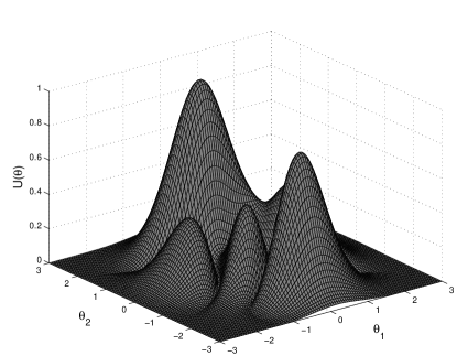
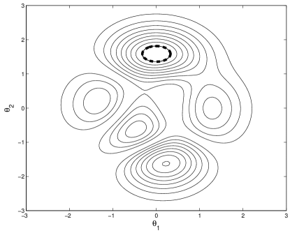
Figure 3: Function $U(\theta)$ (left panel) and its level sets (right panel). The $0.9$ level set is highlighted as a dashed ellipse.

To obtain a stochastic programming problem multiplicative noise was added using the function

$$g(\bm{x},\theta)=(1+\bm{x})U(\theta)$$

where $\bm{x}$ is normally distributed with mean $0$ and variance $0.25$. It is easy to see that the expected value of $g(\bm{x},\theta)$ is indeed equal to $U(\theta)$. One can think of $g(\bm{x},\theta)$ as an imperfect, unbiased measurement device of $U(\theta)$: We can only collect information about $U$ through noise corrupted samples generated by $g$. Notice that the noise intensity is higher in areas where $U(\theta)$ is large, making it more difficult to use the samples to pinpoint the maxima of $U$.

The MCMC Algorithm II of Fig. 1 was applied to this function. The design parameter $\delta=0.1$ and an independent uniform proposal distribution $q$ were used throughout.

To demonstrate the convergence of the algorithm, $2,000$ independent runs of the algorithm, of $10,000$ steps each, were generated. We then computed the fraction of runs that found themselves in $\Theta^{*}(0.1)$ at different time points; for simplicity we refer to this fraction as the ‘success rate’. The results for different values of $J$ are reported in the left panel of Fig. 4. It is clear that in all cases the success rate quickly settles to a steady state value, suggesting that the algorithm has converged. Moreover, the steady state success rate increases as $J$ increases. In the right panel of Fig. 4 we concentrate on the case $J=100$ and plot in a logarithmic scale the absolute value of the difference between the success rate at different time points and the steady state success rate. According to Theorem 7, one would expect this difference to decay to $0$ geometrically at a rate $1-\frac{1}{M}$. For comparison purposes, the corresponding curve for the numerically estimated value $M=1475$, is also plotted on the figure. The bound of Theorem 7 indeed appears to be valid, albeit, in this case, conservative.

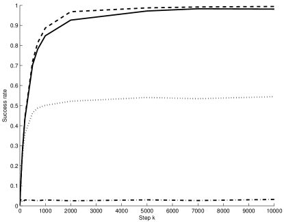
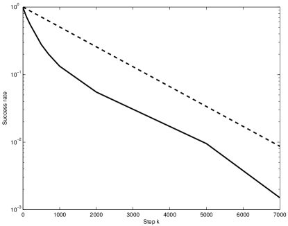
Figure 4: Left panel: Success rate as a function of simulation step for $J=1$ (dot-dash), $J=10$ (dotted), $J=100$ (solid) and $J=200$ (dashed). Right panel: Logarithmic plot of success rate for $J=100$ (solid) with bound of Theorem 7 (dashed).

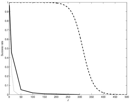
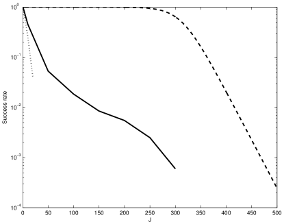
Figure 5: Plot of the decay of $1$ minus the success rate as a function of the exponent $J$ in linear (left panel) and logarithmic (right panel) scales. Both plots show the empirical value based on the last state of $2,000$ independent runs of $10,000$ steps each (solid), the empirical value based on the last $2,000$ states of a single $10,000$ step run (dotted), and the theoretical bound (dashed). $5,000$ independent runs were used for the case $J=300$, since the first $2,000$ runs all ended up in $\Theta^{*}(0.1)$ at step $10,000$.

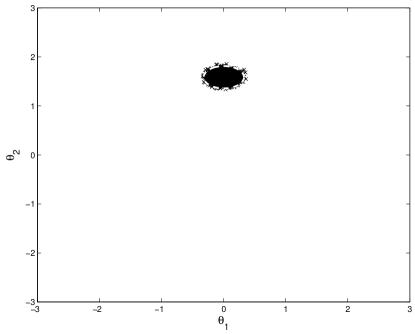
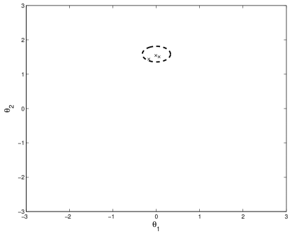
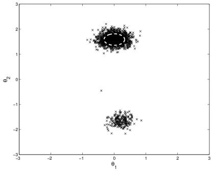
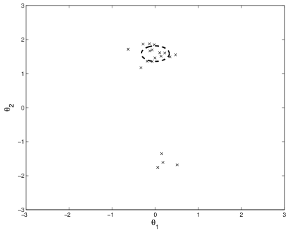
Figure 6: Location of the the last state of $2,000$ independent runs of $10,000$ steps each (left column) and the last $2,000$ steps of a single $10,000$ step run (right column) for $J=100$ (top row) and $J=10$ (bottom row). The set $\Theta^{*}(0.1)$ is plotted as a dashed ellipse for comparison.

To demonstrate the bound of Proposition 5 the steady state success rate as a function of the exponent $J$ is reported in Fig. 5; more precisely, the figure shows the decay of $1$ minus the steady state success rate as a function of $J$ in linear and logarithmic scales. The figure also shows the corresponding theoretical bound based on Proposition 5. Once again the bound appears to be valid. Finally, notice that although in this particular case the proposal distribution is an independent uniform distribution, the resulting states of the chain are a sequence of dependent samples. In Fig. 5 we show the success rate estimated using the last $2,000$ states of a single MCMC run of length $10,000$ (instead of the last state of $2,000$ independent MCMC runs of length $10,000$ each). It appears that the success rate increases much faster in this case. This is due to the fact that the $2,000$ samples used are now correlated. Figure 6 demonstrates this through a scatter plots of the location of the $2,000$ states used to estimate the success rate for $J=100$ in the two cases. While for both the $2,000$ independent runs and the single run most of the states end up inside the set $\Theta^{*}(0.1)$ as expected, it is apparent that the chain only moves three times in the last $2,000$ steps of the single run; all other proposals are rejected. Plots for the case $J=10$ are also included. Note that in this case points near the second largest local maximum are also occasionally accepted.

VI Comparison with other approaches to stochastic optimization

In this section we attempt a comparison between the computational features of the MCMC approach with those of other state-of-the-art methods for solving the stochastic programming problem (2) with finite-time performance bounds. Other methods are typically formulated under the assumption that the distribution $P_{\bm{x}}(\cdot;\theta)$ does not depend on $\theta$. In this case, $U$ becomes

$$U(\theta)=\int g(x,\theta)P_{\bm{x}}(dx).$$ (14)

We stress from the beginning that a direct comparison of the computational complexity of the different methods is not possible at this stage, since the different methods rely on different assumptions, e.g. some methods require solving an additional optimization problem. Moreover, a satisfactory complexity analysis for the MCMC approach is not yet available. The comparison focuses on the number of samples of $\bm{x}$ required in each method to obtain an approximate value optimizer with imprecision $2\epsilon$, with confidence $\rho$, in the optimization of (14). In Table I we compare the growth rates of the total number of samples of $\bm{x}$ required in each method to obtain the desired optimization accuracy as a function of the parameters of the problem.

In the approach of Shapiro [30, 31], $N$ independent samples $\bm{x}_{1},\ldots,\bm{x}_{N}$, generated according to $P_{\bm{x}}$, are used to construct the approximate criterion

$$\hat{U}(\theta)=\frac{1}{N}\sum_{i=1}^{N}g(\bm{x}_{i},\theta).$$ (15)

It is shown in [30, 31] that if $\hat{\bm{\theta}}_{S}$ is an approximate value optimizer of $\hat{U}$ with imprecision $\epsilon$ then $\hat{\bm{\theta}}_{S}$ is also an approximate value optimizer of $U$ with imprecision $2\epsilon$ with probability at least $\rho$, provided that $N$ is sufficiently high. The growth rates of the required $N$, reported in the first line of Table I, are based on [31, equation (3.9)]. Notice that this is only a bound on the samples required to construct $\hat{U}$. It is argued in [31] that the optimization of $\hat{U}$ within $\epsilon$ of optimality can be carried out efficiently under convexity assumptions. Nesterov [32, 33] presents a specific approach for convex stochastic problems. In this approach the samples generated according to $P_{\bm{x}}$ are used to construct an estimate of the optimizer of $U$ using a stochastic sub-gradient algorithm. The growth rates of the number of samples required to obtain an approximate value optimizer of $U$ with imprecision $2\epsilon$ with probability at least $\rho$, are reported in the second line of Table I and are based on [33, equation (14)]. Finally Vidyasagar [22, 20] proposed a fully randomized algorithm which, as mentioned earlier, is closely related to the one presented in our work. In Vidyasagar’s approach one generates $N$ independent samples $\bm{\theta}_{1},\ldots,\bm{\theta}_{N}$ according to a ‘search’ distribution $P_{\bm{\theta}}$, which has support on $\Theta$, and $M$ independent samples $\bm{x}_{1},\ldots,\bm{x}_{M}$ according to $P_{\bm{x}}$, and sets

$$\hat{\bm{\theta}}_{V}=\arg\min_{i=1,\ldots,N}\frac{1}{M}\sum_{j=1}^{M}g(\bm{x}_{j},\bm{\theta}_{i}).$$ (16)

Under minimal assumptions, close to our Assumption 1, it can be shown that if

$$N\geq\frac{\mbox{$\displaystyle\log\frac{2}{1-\rho}$}}{\mbox{$\displaystyle\log\frac{1}{1-\alpha}$}}\quad\mbox{ and }\quad M\geq\frac{1}{2\epsilon^{2}}\log\frac{4N}{1-\rho},$$ (17)

then

$$P_{\bm{\theta}}(\{\theta\in\Theta\;|\;U(\theta)>U(\hat{\bm{\theta}}_{V})+\epsilon\})\leq\alpha$$ (18)

with probability at least $\rho$. It is shown in [20] that potentially tighter bounds can be obtained if the family of functions $\{g(\cdot,\theta)\;|\;\theta\in\Theta\}$ has the UCEM property. Notice that (18) resembles (3) in our definition of approximate domain optimizer. The difference is that the measure of the set of points which are $\epsilon$ better than the candidate optimizer is taken with respect to $P_{\bm{\theta}}$ in (18) as opposed to the Lebesgue measure in (3). If, and only if, $P_{\bm{\theta}}$ is chosen to be the uniform distribution over $\Theta$ then (18) becomes virtually equivalent to (3). In this case, we can apply Theorem 1 and obtain the number of samples required to obtain an approximate value optimizer. By substituting $\alpha$ with the right-hand side of (6) in (17) we obtain that if

$$N\geq\left(\frac{LR}{\epsilon}\right)^{n}\log\frac{2}{1-\rho}\quad\mbox{ and }\quad M\geq\frac{1}{2\epsilon^{2}}\left[\log\frac{4}{1-\rho}+\log\log\frac{2}{1-\rho}+n\log\frac{LR}{\epsilon}\right]$$ (19)

then $\hat{\theta}_{V}$ is an approximate value optimizer of $U$ with imprecision $2\epsilon$ with probability at least $\rho$. Notice that now the number of samples on $\Theta$ turns out to be exponential in $n$.

		$\displaystyle\epsilon$		$\displaystyle\rho\mbox{ or }\sigma$		$\displaystyle LR$		$\displaystyle n$		problem
Shapiro [30, 31]		$\displaystyle\frac{1}{\epsilon^{2}}\log\frac{1}{\epsilon}$		$\displaystyle\log\frac{1}{1-\rho}$		$\displaystyle(LR)^{2}\log LR$		$\displaystyle n$		convex
Nesterov [32, 33]		$\displaystyle\frac{1}{\epsilon^{4}}$		$\displaystyle\log\frac{1}{1-\rho}$		$\displaystyle(LR)^{2}$		$\displaystyle-$		convex
Vidyasagar (19)		$\displaystyle\frac{1}{\epsilon^{2}}\log\frac{1}{\epsilon}$		$\displaystyle\log\frac{1}{1-\rho}$		$\displaystyle\log LR$		$\displaystyle n$		general
MCMC (10) [per iteration]		$\displaystyle\frac{1}{\epsilon}\log\frac{1}{\epsilon}$		$\displaystyle\log\frac{1}{1-\sigma}$		$\displaystyle\log LR$		$\displaystyle n$		general

TABLE I: Growth rates of the number of samples of $\bm{x}$ required to obtain an approximate value optimizer with imprecision $2\epsilon$ of $U$, given by (14), with probability $\rho$. In the case of MCMC, the entries of the table represent the number of samples of $\bm{x}$ required to perform one iteration of the algorithm.

In the last row of the table, we have included the growth rates of (10), which is the number of samples of $\bm{x}$ which must be generated at each iteration of Algorithm II (which coincides with the exponent $J$). In this case, the total number of required samples of $\bm{x}$ is $J$ times the number of iterations required to achieve the desired reduction of $\|P_{\bm{\theta}_{k}}-\pi(\,\cdot\,\,;J,\delta)\|_{\mbox{\tiny TV}}$. Hence, the entries of the last row represent a lower bound, or the ‘base-line’ growth rates, of the total number of required samples in the MCMC approach. In this case, the confidence is $\rho=\sigma-\|P_{\bm{\theta}_{k}}-\pi(\,\cdot\,\,;J,\delta)\|_{\mbox{\tiny TV}}$. Hence, since $\sigma>\rho$, it is sensible to consider the growth rate with respect to $\sigma$ instead of $\rho$. By comparing the different entries in the table, we notice that (10) grows slower than or at the same rate as the other bounds. Overall, the comparison reveals that in principle there is scope for obtaining MCMC algorithm which, in terms of numbers of required samples of $\bm{x}$, have a computational cost comparable to those of the other approaches. Here we present a preliminary complexity analysis which shows that the introduction of a cooling schedule would eventually lead to efficient algorithms. Notice that in Section IV we considered a constant schedule ($J_{k}=J$). Here, we assume that $J_{k}$ takes integer values starting with $J_{1}=1$ and ending with $J_{k}=J$, where $J$ is the smallest integer which satisfies either (9) or (10). In the earliest works on simulated annealing, the logarithmic schedule of the type $J_{k}=\lfloor\log k\rfloor+1$ was often adopted [13, 14, 17]. Here, we are interested in counting the total number of iterations required to complete the cooling schedule when $J$ is given by (9) or (10). Let $K_{i}$ denote the number of iterations in which $J_{k}=i$ for each $i=1,2,\dots,J$. Hence, the total number of iterations is $\sum_{i=1}^{J}K_{i}$ and, in Algorithm II, the total number of required samples of $\bm{x}$ would be $\sum_{i=1}^{J}iK_{i}$. For the logarithmic schedule $J_{k}=\lfloor\log k\rfloor+1$ we have $K_{i}=\lfloor e^{i}\rfloor-\lfloor e^{i-1}\rfloor$. Hence we obtain

$$\sum_{i=1}^{J}K_{i}=\sum_{i=1}^{J}\lfloor e^{i}\rfloor-\lfloor e^{i-1}\rfloor\approx e^{J}-1\,,\qquad\sum_{i=1}^{J}iK_{i}\approx Je^{J}-\frac{1-e^{J}}{1-e}.$$

In this case the number of iterations turns out to be exponential in $\frac{1}{\epsilon}$. Hence, a logarithmic schedule is not sufficient to obtain efficient algorithms.

In more recent works [15, 16, 19], the faster algebraic schedule of the type $J_{k}=\lfloor k^{a}\rfloor$, with $a>0$, has been considered. It is shown in [15, 16, 19] that the choice of the faster algebraic schedule requires a sophisticated design of the proposal distribution. For the algebraic schedule $J_{k}=\lfloor k^{a}\rfloor$ we have $K_{i}=\lfloor(i+1)^{\frac{1}{a}}\rfloor-\lfloor i^{\frac{1}{a}}\rfloor$. Hence we obtain

$$\sum_{i=1}^{J}K_{i} = \sum_{i=1}^{J}\lfloor(i+1)^{\frac{1}{a}}\rfloor-\lfloor i^{\frac{1}{a}}\rfloor\approx\left(J+1\right)^{\frac{1}{a}}-1\,,$$

$$\sum_{i=1}^{J}iK_{i} \approx J\left(J+1\right)^{\frac{1}{a}}-\sum_{i=0}^{J-1}\left(i+1\right)^{\frac{1}{a}}.$$

In this case the number of iterations grows as $J^{\frac{1}{a}}$. Hence, in the case of approximate domain optimization, where $J$ is given by (9), the number of iterations grows as $(\frac{1}{\epsilon})^{\frac{1}{a}}$, $(\log\frac{1}{\alpha})^{\frac{1}{a}}$ and $(\log\frac{1}{1-\sigma})^{\frac{1}{a}}$. In the case of approximate value optimization, where $J$ is given by (10), the number of iterations grows as $(\frac{1}{\epsilon}\log\frac{1}{\epsilon})^{\frac{1}{a}}$, $(\log\frac{1}{1-\sigma})^{\frac{1}{a}}$, $(\log LR)^{\frac{1}{a}}$ and $n^{\frac{1}{a}}$. In Algorithm II, the total number of samples of $\bm{x}$ is given by the number of iterations multiplied by $J$. Hence, in the case of approximate domain optimization, it grows as $(\frac{1}{\epsilon})^{1+\frac{1}{a}}$, $(\log\frac{1}{\alpha})^{1+\frac{1}{a}}$ and $(\log\frac{1}{1-\sigma})^{1+\frac{1}{a}}$. In the case of approximate value optimization, it grows as $(\frac{1}{\epsilon}\log\frac{1}{\epsilon})^{1+\frac{1}{a}}$, $(\log\frac{1}{1-\sigma})^{1+\frac{1}{a}}$, $(\log LR)^{1+\frac{1}{a}}$ and $n^{1+\frac{1}{a}}$ (notice that, as $a$ increases, the growth rates approach the entries of the last row of Table I). Hence, an algebraic schedule leads to algorithms with polynomial growth rates. The convergence analysis of Algorithms I and II with an additional algebraic cooling schedule goes beyond the scope of this paper. Here, we limit ourselves to pointing out that the choice of a target distribution $\pi(\,\cdot\,\,;J,\delta)$ with a finite $J$ implies that the cooling schedule $\{J_{k}\}_{k=1,2,\dots}$ can be chosen to be a sequence that takes only a finite set of values. In turn, this fact should make the study of convergence of $P_{\bm{\theta}_{k}}$ to $\pi(\,\cdot\,\,;J,\delta)$ in total variation distance easier than the study of asymptotic convergence of $P_{\bm{\theta}_{k}}$ to the zero-temperature distribution $\pi_{\infty}$.

VII Conclusions

In this paper, we have introduced a novel approach for obtaining rigorous finite-time guarantees on the performance of MCMC algorithms in the optimization of functions of continuous variables. In particular we have established the values of the the temperature parameter in the target distribution which allow one to reach a solution, which is within the desired level of approximation with the desired confidence, in a finite number of steps. Our work was motivated by the MCMC algorithm (Algorithm II), introduced in [34, 35, 36], for solving stochastic optimization problems. On the basis of our results, we were able to obtain the ‘base-line’ computational complexity of the MCMC approach and to perform an initial assessment of the computational complexity of MCMC algorithms. It has been shown that MCMC algorithms with an algebraic cooling schedule would have polynomial complexity bounds comparable with those of other state-of-the-art methods for solving stochastic optimization problems. Conditions for asymptotic convergence of simulated annealing algorithms with an algebraic cooling schedule have already been reported in the literature [15, 16, 19]. Our results enable novel research on the development of efficient MCMC algorithms for the solution of stochastic programming problems with rigorous finite-time guarantees. Finally, we would like to point out that the results presented in this work do not apply to the MCMC approach only but do apply also to other sampling methods which can implement the idea of simulated annealing [46, 47].

Acknowledgments

Work supported by EPSRC, Grant EP/C014006/1, and by the European Commission under projects HYGEIA FP6-NEST-4995 and iFly FP6-TREN-037180.

In order to prove Theorem 1 we first need to prove a preliminary technical result.

Lemma 10

For $A\subseteq{\mathbb{R}}^{n}$ and $\theta\in{\mathbb{R}}^{n}$ let $d(\theta,A):=\inf_{\theta^{\prime}\in A}\|\theta-\theta^{\prime}\|.$ Then, for any $\beta\geq 0$

$$d^{*}_{\beta}:=\sup_{\tiny\begin{array}[]{c}A\subseteq{\mathbb{R}}^{n}\\ \lambda(A)\leq\beta\end{array}}\sup_{\theta\in A}d(\theta,A^{c})=\frac{1}{\sqrt{\pi}}\left[\frac{n}{2}\Gamma\left(\frac{n}{2}\right)\right]^{\frac{1}{n}}\beta^{\frac{1}{n}}$$

where $A^{c}$ denotes the complement of $A$ in ${\mathbb{R}}^{n}$.

In the above Lemma the inner supremum determines the points in the set $A$ whose distance from the complement of $A$ is the largest; loosely speaking the points that lie the furthest from the boundary of $A$ or the deepest in the interior of $A$. The outer supremum then maximizes this distance over all sets $A$ whose Lebesgue measure is bounded by $\beta$.

Proof: We show that the optimizers for the outer supremum are 2-norm balls in ${\mathbb{R}}^{n}$; then, the inner supremum is achieved by the center of the ball.

Consider any set $A\subseteq{\mathbb{R}}^{n}$ with $\lambda(A)\leq\beta$ and let

$$d_{A}:=\sup_{\theta\in A}d(\theta,A^{c}).$$ (20)

Since $\lambda(A)<\infty$ , the supremum (20) is achieved by some $\theta_{A}\in A$. Without loss of generality we can assume that the set $A$ is closed; if not, taking its closure will not affect its Lebesgue measure and will lead to the same value for $d_{A}$. Let $B(\theta,d)$ denote the 2-norm ball with center in $\theta$ and radius $d$. Notice that by construction $B(\theta_{A},d_{A})\subseteq A$ and therefore $\lambda(B(\theta_{A},d_{A}))\leq\lambda(A)\leq\beta$. Moreover,

$$\sup_{\theta\in B(\theta_{A},d_{A})}d(\theta,B(\theta_{A},d_{A})^{c})=d_{A}$$

achieved at the center, $\theta_{A}$, of the ball. In summary, for any $A\subseteq{\mathbb{R}}^{n}$ with $\lambda(A)\leq\beta$ one can find a 2-norm ball of measure at most $\beta$ which achieves $\sup_{\theta\in A}d(\theta,A^{c})$.

Therefore,

$$d^{*}_{\beta}: =\sup_{\tiny\begin{array}[]{c}A\subseteq{\mathbb{R}}^{n}\\ \lambda(A)\leq\beta\end{array}}\sup_{\theta\in A}d(\theta,A^{c})$$

$$=\sup_{\tiny\begin{array}[]{c}(\theta^{\prime},r)\in{\mathbb{R}}^{n}\times{\mathbb{R}}_{+}\\ \lambda(B(\theta^{\prime},r))\leq\beta\end{array}}\sup_{\theta\in B(\theta^{\prime},r)}d(\theta,B(\theta^{\prime},r)^{c})$$

$$=\sup_{\tiny\begin{array}[]{c}r\geq 0\\ \lambda(B(0,r))\leq\beta\end{array}}\sup_{\theta\in B(0,r)}d(\theta,B(0,r)^{c})$$

$$=\sup_{\tiny\begin{array}[]{c}r\geq 0\\ \lambda(B(0,r))\leq\beta\end{array}}r$$

$$=\frac{1}{\sqrt{\pi}}\left[\frac{n}{2}\Gamma\left(\frac{n}{2}\right)\right]^{\frac{1}{n}}\beta^{\frac{1}{n}}.$$

In the above derivation, the last equality is obtained by recalling that $\displaystyle\lambda(B(\theta,r))=\frac{2\pi^{\frac{n}{2}}}{n\Gamma(\frac{n}{2})}r^{n}$.   

We are now in a position to prove Theorem 1.

Proof of Theorem 1: Let $\hat{\Theta}(\theta,\epsilon):=\{\theta^{\prime}\in\Theta\;|\;U(\theta^{\prime})>U(\theta)+\epsilon\}$ and recall that by definition

$$\lambda(\hat{\Theta}(\theta,\epsilon))\leq\alpha\,\lambda(\Theta)\,.$$

Take any $\tilde{\theta}\in\Theta$. Then either $U(\tilde{\theta})\leq U(\theta)+\epsilon$ or $\tilde{\theta}\in\hat{\Theta}(\theta,\epsilon)$. In the former case there is nothing to prove. In the latter case, according to Lemma 10, we have:

$$d(\tilde{\theta},\hat{\Theta}(\theta,\epsilon)^{c})\leq\frac{1}{\sqrt{\pi}}\left[\frac{n}{2}\Gamma\left(\frac{n}{2}\right)\right]^{\frac{1}{n}}[\alpha\lambda(\Theta)]^{\frac{1}{n}}.$$

Since $\Theta$ is compact and $U$ is continuous, the set $\hat{\Theta}(\theta,\epsilon)^{c}$ is closed and therefore there exists $\bar{\theta}\in\hat{\Theta}(\theta,\epsilon)^{c}$ such that

$$\|\tilde{\theta}-\bar{\theta}\|\leq\frac{1}{\sqrt{\pi}}\left[\frac{n}{2}\Gamma\left(\frac{n}{2}\right)\right]^{\frac{1}{n}}[\alpha\lambda(\Theta)]^{\frac{1}{n}}.$$

Moreover, since $U$ is Lipschitz, $|U(\tilde{\theta})-U(\bar{\theta})|\leq L\|\tilde{\theta}-\bar{\theta}\|$. Since $\bar{\theta}\in\hat{\Theta}(\hat{\theta},\epsilon)^{c}$, we have that $U(\bar{\theta})\leq U(\theta)+\epsilon$, and therefore

$$U(\tilde{\theta})\leq U(\theta)+\epsilon+\frac{L}{\sqrt{\pi}}\left[\frac{n}{2}\Gamma\left(\frac{n}{2}\right)\right]^{\frac{1}{n}}[\alpha\lambda(\Theta)]^{\frac{1}{n}}.$$ (21)

The claim follows since $\tilde{\theta}$ is arbitrary in $\Theta$ and satisfies either $U(\tilde{\theta})\leq U(\theta)+\epsilon$ or (21).   

Proof of Theorem 2: Let ${\bar{\alpha}}\in(0,1]$ and $\rho\in(0,1]$ be given numbers. To simplify the notation, let $U_{\delta}(\theta):=U(\theta)+\delta$ and let $\pi_{\delta}$ be a normalized measure such that $\pi_{\delta}(d\theta)\propto U_{\delta}(\theta)\lambda(d\theta)$, i.e. $\pi_{\delta}(d\theta):=\pi(d\theta;1,\delta)$. In the first part of the proof we establish a lower bound on

$$\pi\left(\{\theta\in\Theta\;|\;\pi_{\delta}(\{\theta^{\prime}\in\Theta\;|\;\rho\,U_{\delta}(\theta^{\prime})>U_{\delta}(\theta)\})\leq{\bar{\alpha}}\};J,\delta\right)\,.$$

Let $y_{\bar{\alpha}}:=\inf\{y\;|\;\pi_{\delta}(\{\theta\in\Theta\;|\;U_{\delta}(\theta)\leq y\})\geq 1-{\bar{\alpha}}\}$. To start with we show that the set $\{\theta\in\Theta\;|\;\pi_{\delta}(\{\theta^{\prime}\in\Theta\;|\;\rho\,U_{\delta}(\theta^{\prime})>U_{\delta}(\theta)\})\leq{\bar{\alpha}}\}$ coincides with $\{\theta\in\Theta\;|\;U_{\delta}(\theta)\geq\rho\,y_{\bar{\alpha}}\}$. Notice that the quantity $\pi_{\delta}(\{\theta\in\Theta\;|\;U_{\delta}(\theta)\leq y\})$ is a non decreasing right continuous function of $y$ because it has the form of a distribution function (see e.g. [48, p. 162], see also [22, Lemma 11.1]). Therefore we have $\pi_{\delta}(\{\theta\in\Theta\;|\;U_{\delta}(\theta)\leq y_{\bar{\alpha}}\})\geq 1-{\bar{\alpha}}$ and

$$y\geq\rho\,y_{\bar{\alpha}}\,\Rightarrow\,\pi_{\delta}(\{\theta^{\prime}\in\Theta\;|\;\rho\,U_{\delta}(\theta^{\prime})\leq y\})\geq 1-{\bar{\alpha}}\,\Rightarrow\,\pi_{\delta}(\{\theta^{\prime}\in\Theta\;|\;\rho\,U_{\delta}(\theta^{\prime})>y\})\leq{\bar{\alpha}}\,.$$

Moreover,

$$y<\rho\,y_{\bar{\alpha}}\,\Rightarrow\,\pi_{\delta}(\{\theta^{\prime}\in\Theta\;|\;\rho\,U_{\delta}(\theta^{\prime})\leq y\})<1-{\bar{\alpha}}\,\Rightarrow\,\pi_{\delta}(\{\theta^{\prime}\in\Theta\;|\;\rho\,U_{\delta}(\theta^{\prime})>y\})>{\bar{\alpha}}\,$$

and taking the contrapositive one obtains

$$\pi_{\delta}(\{\theta^{\prime}\in\Theta\;|\;\rho\,U_{\delta}(\theta^{\prime})>y\})\leq{\bar{\alpha}}\quad\Rightarrow\quad y\geq\rho\,y_{\bar{\alpha}}\,.$$

Therefore $\{\theta\in\Theta\;|\;U_{\delta}(\theta)\geq\rho\,y_{\bar{\alpha}}\}=\{\theta\in\Theta\;|\;\pi_{\delta}(\{\theta^{\prime}\in\Theta\;|\;\rho\,U_{\delta}(\theta^{\prime})>U_{\delta}(\theta)\})\leq{\bar{\alpha}}\}$.

We now derive a lower bound on $\pi\left(\{\theta\in\Theta\;|\;U_{\delta}(\theta)\geq\rho\,y_{\bar{\alpha}}\};J,\delta\right)$. Let us introduce the notation $A_{\bar{\alpha}}:=\{\theta\in\Theta\;|\;U_{\delta}(\theta)<y_{\bar{\alpha}}\}$, $\bar{A}_{\bar{\alpha}}:=\{\theta\in\Theta\;|\;U_{\delta}(\theta)\geq y_{\bar{\alpha}}\}$, $B_{{\bar{\alpha}},\rho}:=\{\theta\in\Theta\;|\;U_{\delta}(\theta)<\rho\,y_{\bar{\alpha}}\}$ and $\bar{B}_{{\bar{\alpha}},\rho}:=\{\theta\in\Theta\;|\;U_{\delta}(\theta)\geq\rho\,y_{\bar{\alpha}}\}$. Notice that $B_{{\bar{\alpha}},\rho}\subseteq A_{\bar{\alpha}}$ and $\bar{A}_{\bar{\alpha}}\subseteq\bar{B}_{{\bar{\alpha}},\rho}$. The quantity $\pi_{\delta}(\{\theta\in\Theta\;|\;U_{\delta}(\theta)<y\})$ as a function of $y$ is the left continuous version of $\pi_{\delta}(\{\theta\in\Theta\;|\;U_{\delta}(\theta)\leq y\})$ [48, p. 162]. Hence, the definition of $y_{\bar{\alpha}}$ implies $\pi_{\delta}(A_{\bar{\alpha}})\leq 1-{\bar{\alpha}}$ and $\pi_{\delta}(\bar{A}_{\bar{\alpha}})\geq{\bar{\alpha}}$. Notice that

$$\pi_{\delta}(A_{\bar{\alpha}})\leq 1-{\bar{\alpha}}\quad \Rightarrow\quad\frac{\delta\lambda(A_{\bar{\alpha}})}{\left[\int_{\Theta}U_{\delta}(\theta)\lambda(d\theta)\right]}\leq 1-{\bar{\alpha}}\qquad\mbox{ because }U(\theta)\geq 0\;\forall\theta\,,$$

$$\pi_{\delta}(\bar{A}_{\bar{\alpha}})\geq{\bar{\alpha}}\quad \Rightarrow\quad\frac{(1+\delta)\lambda(\bar{A}_{\bar{\alpha}})}{\left[\int_{\Theta}U_{\delta}(\theta)\lambda(d\theta)\right]}\geq{\bar{\alpha}}\qquad\qquad\mbox{because }U(\theta)\leq 1\;\forall\theta\,.$$

Hence, ${\lambda(\bar{A}_{\bar{\alpha}})}>0$ and

$$\frac{\lambda(A_{\bar{\alpha}})}{\lambda(\bar{A}_{\bar{\alpha}})}\leq\frac{1-{\bar{\alpha}}}{{\bar{\alpha}}}\frac{1+\delta}{\delta}\,.$$

Notice that ${\lambda(\bar{A}_{\bar{\alpha}})}>0$ implies ${\lambda(\bar{B}_{{\bar{\alpha}},\rho})}>0$. We obtain

$$\pi\left(\{\theta\in\Theta\;|\;U_{\delta}(\theta)\geq\rho\,y_{\bar{\alpha}}\};J,\delta\right) = \pi\left(\bar{B}_{{\bar{\alpha}},\rho};J,\delta\right)=\frac{\int_{\bar{B}_{{\bar{\alpha}},\rho}}U_{\delta}(\theta)^{J}\lambda(d\theta)}{\int_{\Theta}U_{\delta}(\theta)^{J}\lambda(d\theta)}$$

$$= \frac{\int_{\bar{B}_{{\bar{\alpha}},\rho}}U_{\delta}(\theta)^{J}\lambda(d\theta)}{\int_{B_{{\bar{\alpha}},\rho}}U_{\delta}(\theta)^{J}\lambda(d\theta)+\int_{\bar{B}_{{\bar{\alpha}},\rho}}U_{\delta}(\theta)^{J}\lambda(d\theta)}$$

$$= \frac{1}{\mbox{$\displaystyle 1+\frac{\int_{B_{{\bar{\alpha}},\rho}}U_{\delta}(\theta)^{J}\lambda(d\theta)}{\int_{\bar{B}_{{\bar{\alpha}},\rho}}U_{\delta}(\theta)^{J}\lambda(d\theta)}$}}$$

$$\geq \frac{1}{\mbox{$\displaystyle 1+\frac{\int_{B_{{\bar{\alpha}},\rho}}U_{\delta}(\theta)^{J}\lambda(d\theta)}{\int_{\bar{A}_{\bar{\alpha}}}U_{\delta}(\theta)^{J}\lambda(d\theta)}$}}$$

$$\geq \frac{1}{\mbox{$\displaystyle 1+\frac{\rho^{\,J}y_{\bar{\alpha}}^{J}}{y_{\bar{\alpha}}^{J}}\frac{\lambda(B_{{\bar{\alpha}},\rho})}{\lambda(\bar{A}_{\bar{\alpha}})}$}}$$

$$\geq \frac{1}{\mbox{$\displaystyle 1+\rho^{\,J}\frac{\lambda(A_{\bar{\alpha}})}{\lambda(\bar{A}_{\bar{\alpha}})}$}}$$

$$\geq \frac{1}{\mbox{$\displaystyle 1+\rho^{\,J}\frac{1-{\bar{\alpha}}}{{\bar{\alpha}}}\frac{1+\delta}{\delta}$}}\,.$$

Since $\{\theta\in\Theta\;|\;U_{\delta}(\theta)\geq\rho\,y_{\bar{\alpha}}\}=\{\theta\in\Theta\;|\;\pi_{\delta}(\{\theta^{\prime}\in\Theta\;|\;\rho\,U_{\delta}(\theta^{\prime})>U_{\delta}(\theta)\})\leq{\bar{\alpha}}\}$ the first part of the proof is complete.

In the second part of the proof we show that the set $\{\theta\in\Theta\;|\;\pi_{\delta}(\{\theta^{\prime}\in\Theta\;|\;\rho\,U_{\delta}(\theta^{\prime})>U_{\delta}(\theta)\})\leq{\bar{\alpha}}\}$ is contained in the set of approximate domain optimizers of $U$ with value imprecision $\tilde{\epsilon}:=(\rho^{-1}-1)(1+\delta)$ and residual domain $\tilde{\alpha}:=\frac{1+\delta}{\tilde{\epsilon}+\delta}\,{\bar{\alpha}}$. Hence, we show that

$$\{\theta\in\Theta\;|\;\pi_{\delta}(\{\theta^{\prime}\in\Theta\;|\;\rho\,U_{\delta}(\theta^{\prime})>U_{\delta}(\theta)\})\leq{\bar{\alpha}}\}\subseteq$$

$$\{\theta\in\Theta\;|\;\lambda(\{\theta^{\prime}\in\Theta\;|\;U(\theta^{\prime})>U(\theta)+\tilde{\epsilon}\})\leq\tilde{\alpha}\,\lambda(\Theta)\}\,.$$

We have

$$U(\theta^{\prime})>U(\theta)+\tilde{\epsilon}\quad\Leftrightarrow\quad\rho\,U_{\delta}(\theta^{\prime})>\rho\,[U_{\delta}(\theta)+\tilde{\epsilon}]\quad\Rightarrow\quad\rho\,U_{\delta}(\theta^{\prime})>U_{\delta}(\theta)$$

which is proven by noticing that

$$\rho\,[U_{\delta}(\theta)+\tilde{\epsilon}]\geq U_{\delta}(\theta)\,\,\Leftrightarrow\,\,(1-\rho)\geq U(\theta)(1-\rho)$$

and $U(\theta)\in[0,\,1]$. Hence,

$$\{\theta^{\prime}\in\Theta\;|\;\rho\,U_{\delta}(\theta^{\prime})>U_{\delta}(\theta)\}\quad\supseteq\quad\{\theta^{\prime}\in\Theta\;|\;U(\theta^{\prime})>U(\theta)+\tilde{\epsilon}\}\,.$$

Therefore,

$$\pi_{\delta}(\{\theta^{\prime}\in\Theta\;|\;\rho\,U_{\delta}(\theta^{\prime})>U_{\delta}(\theta)\})\leq{\bar{\alpha}}\quad\Rightarrow\quad\pi_{\delta}(\{\theta^{\prime}\in\Theta\;|\;U(\theta^{\prime})>U(\theta)+\tilde{\epsilon}\})\leq{\bar{\alpha}}\,.$$

Let $Q_{\theta,\tilde{\epsilon}}:=\{\theta^{\prime}\in\Theta\;|\;U(\theta^{\prime})>U(\theta)+\tilde{\epsilon}\}$ and notice that

$$\pi_{\delta}(\{\theta^{\prime}\in\Theta\;|\;U(\theta^{\prime})>U(\theta)+\tilde{\epsilon}\})\,=\,\frac{\mbox{$\displaystyle\int_{Q_{\theta,\tilde{\epsilon}}}U(\theta^{\prime})\lambda(d\theta^{\prime})+\delta\lambda(Q_{\theta,\tilde{\epsilon}})$}}{\mbox{$\displaystyle\int_{\Theta}U(\theta^{\prime})\lambda(d\theta^{\prime})+\delta\lambda(\Theta)$}}\,.$$

We obtain

$$\pi_{\delta}(\{\theta^{\prime}\in\Theta\;|\;U(\theta^{\prime})>U(\theta)+\tilde{\epsilon}\})\leq{\bar{\alpha}}\, \Rightarrow\,\tilde{\epsilon}\,\lambda(Q_{\theta,\tilde{\epsilon}})+\delta\lambda(Q_{\theta,\tilde{\epsilon}})\leq{\bar{\alpha}}(1+\delta)\lambda(\Theta)$$

$$\Rightarrow\,\lambda(\{\theta^{\prime}\in\Theta\;|\;U(\theta^{\prime})>U(\theta)+\tilde{\epsilon}\})\leq\tilde{\alpha}\,\lambda(\Theta)\,.$$

Hence we can conclude that

$$\pi_{\delta}(\{\theta^{\prime}\in\Theta\;|\;\rho\,U_{\delta}(\theta^{\prime})>U_{\delta}(\theta)\})\leq{\bar{\alpha}}\,\,\Rightarrow\,\,\lambda(\{\theta^{\prime}\in\Theta\;|\;U(\theta^{\prime})>U(\theta)+\tilde{\epsilon}\})\leq\tilde{\alpha}\,\lambda(\Theta)$$

and the second part of the proof is complete.

We have shown that given ${\bar{\alpha}}\in(0,\,1]$, $\rho\in(0,\,1]$, $\tilde{\epsilon}:=(\rho^{-1}-1)(1+\delta)$ and $\tilde{\alpha}:=\frac{1+\delta}{\tilde{\epsilon}+\delta}\,{\bar{\alpha}}$, then

$$\pi\left(\Theta(\tilde{\epsilon},\tilde{\alpha});J,\delta\right)\geq\frac{1}{\mbox{$\displaystyle 1+\rho^{\,J}\frac{1-\bar{\alpha}}{\bar{\alpha}}\frac{1+\delta}{\delta}$}}=\frac{1}{\mbox{$\displaystyle 1+\left[\frac{1+\delta}{\tilde{\epsilon}+1+\delta}\right]^{J}\left[\frac{1}{\tilde{\alpha}}\frac{1+\delta}{\tilde{\epsilon}+\delta}-1\right]\frac{1+\delta}{\delta}$}}\,.$$

Notice that $\tilde{\epsilon}\in[0,\,1]$ and $\tilde{\alpha}\in(0,\,1]$ are linked through a bijective relation to $\rho\in[\frac{1+\delta}{2+\delta},\,1]$ and $\bar{\alpha}\in(0,\,\frac{\tilde{\epsilon}+\delta}{1+\delta}]$. Hence, the statement of the theorem is eventually obtained by setting the desired $\tilde{\epsilon}=\epsilon$ and $\tilde{\alpha}=\alpha$ in the above inequality.   

To prove Corollary 3 we will need the following fact.

Proposition 11

For all $x>0$, $y>1$,

$$\log\left(\frac{x+y}{y}\right)\geq\frac{x}{x+y}\,.$$

Proof: Fix an arbitrary $y>1$. If $x=0$ then $\displaystyle\log\frac{x+y}{y}=0=\frac{x}{x+y}$. Moreover,

$$\frac{d}{dx}\left(\frac{x}{x+y}\right)=\frac{y}{(x+y)^{2}}\leq\frac{1}{x+y}=\frac{d}{dx}\left(\log\frac{x+y}{y}\right).$$

 

Proof of Corollary 3: To make sure that $\pi(\Theta(\epsilon,\alpha);J,\delta)\geq\sigma$ we need to select $J$ such that

$$\frac{1}{1+\left[\frac{1+\delta}{\epsilon+1+\delta}\right]^{J}\left[\frac{1}{\alpha}\frac{1+\delta}{\epsilon+\delta}-1\right]\frac{1+\delta}{\delta}}\geq\sigma,$$

or, in other words,

$$\left[\frac{\epsilon+1+\delta}{1+\delta}\right]^{J}\geq\frac{\sigma}{1-\sigma}\left[\frac{1}{\alpha}\frac{1+\delta}{\epsilon+\delta}-1\right]\frac{1+\delta}{\delta}.$$

It therefore suffices to choose $J$ such that

$$\left[\frac{\epsilon+1+\delta}{1+\delta}\right]^{J}\geq\frac{\sigma}{1-\sigma}\frac{1}{\alpha}\left[\frac{1+\delta}{\delta}\right]^{2}.$$

Taking logarithms

$$J\log\frac{\epsilon+1+\delta}{1+\delta}\geq\log\frac{\sigma}{1-\sigma}+\log\frac{1}{\alpha}+2\log\frac{1+\delta}{\delta}.$$

Using the result of Proposition 11 with $x=\epsilon$ and $y=1+\delta$ one eventually obtains that it suffices to select $J$ according to inequality (9).   

Proof of Proposition 6: Notice that

$$\frac{d}{d\delta}f(\delta) =\frac{1}{\epsilon}\left[\log\frac{\sigma}{1-\sigma}+\log\frac{1}{\alpha}+2\log\frac{1+\delta}{\delta}-2\frac{1+\epsilon+\delta}{\delta(1+\delta)}\right]$$

$$\frac{d^{2}}{d\delta^{2}}f(\delta) =2\frac{1+\epsilon+\delta+2\epsilon\delta}{\epsilon\delta^{2}(1+\delta)^{2}}>0$$

and therefore the function $f(\delta)$ is convex in $\delta$. The second equation ensures that if $f(\delta)$ attains a minimum then it is unique. To complete the proof we need to show that the equation

$$\frac{d}{d\delta}f(\delta)=\frac{1}{\epsilon}\left[\log\frac{\sigma}{1-\sigma}+\log\frac{1}{\alpha}+2\log\frac{1+\delta}{\delta}-2\frac{1+\epsilon+\delta}{\delta(1+\delta)}\right]=0$$ (22)

always has a solution for $\delta>0$. To simplify the notation define

$$f_{1}(\delta) =\log\frac{1+\delta}{\delta}+\log\frac{\sqrt{\sigma}}{\sqrt{1-\sigma}}+\log\frac{1}{\sqrt{\alpha}}$$

$$f_{2}(\delta) =\frac{1+\epsilon+\delta}{\delta(1+\delta)}.$$

Then (22) simplifies to $f_{1}(\delta)=f_{2}(\delta)$. It is easy to see that both $f_{1}$ and $f_{2}$ are monotone decreasing functions of $\delta$ and

$$\lim_{\delta\rightarrow 0}f_{1}(\delta) =\lim_{\delta\rightarrow 0}f_{2}(\delta)=\infty,$$

$$\lim_{\delta\rightarrow\infty}f_{1}(\delta) =\log\frac{\sqrt{\sigma}}{\sqrt{1-\sigma}}+\log\frac{1}{\sqrt{\alpha}}>0\mbox{ for $\sigma\in(0.5,\,1)$, }\mbox{ and }\lim_{\delta\rightarrow\infty}f_{2}(\delta)=0.$$

Moreover, as $\delta$ tends to $0$, $f_{1}(\delta)$ tends to infinity more slowly than $f_{2}(\delta)$ ($O(\log(1/\delta)$ instead of $O(1/\delta)$). Therefore the two function have to cross for some $\delta>0$.   

Proof of Proposition 8: Let $p(\cdot;J,\delta)$ denote the density of $\pi(\cdot;J,\delta)$. Consider any $\theta^{*}\in\Theta^{*}$. We have:

$$p(\theta;J,\delta) =\frac{\left[U(\theta)+\delta\right]^{J}}{\int_{\theta^{\prime}\in\Theta}\left[U(\theta^{\prime})+\delta\right]^{J}\lambda(d\theta^{\prime})}$$

$$\leq\frac{\left[U(\theta^{*})+\delta\right]^{J}}{\int_{\theta^{\prime}\in\Theta}\left[U(\theta^{\prime})+\delta\right]^{J}\lambda(d\theta^{\prime})}$$

$$=\frac{\int_{\theta^{\prime}\in\Theta^{*}}\left[U(\theta^{\prime})+\delta\right]^{J}\lambda(d\theta^{\prime})}{\lambda(\Theta^{*})}\frac{1}{\int_{\theta^{\prime}\in\Theta}\left[U(\theta^{\prime})+\delta\right]^{J}\lambda(d\theta^{\prime})}$$

$$\leq\frac{\int_{\theta^{\prime}\in\Theta}\left[U(\theta^{\prime})+\delta\right]^{J}\lambda(d\theta^{\prime})}{\lambda(\Theta^{*})}\frac{1}{\int_{\theta^{\prime}\in\Theta}\left[U(\theta^{\prime})+\delta\right]^{J}\lambda(d\theta^{\prime})}$$

$$=\frac{\lambda(\Theta)}{\lambda(\Theta^{*})}\frac{1}{\lambda(\Theta)}$$

$$\leq\frac{1}{\beta}\frac{1}{\lambda(\Theta)}.$$

Recall that the independent uniform proposal distribution over $\Theta$ has density $q(\theta)=\frac{1}{\lambda(\Theta)}$. Hence, from the above inequality we obtain that $M=\frac{1}{\beta}$ satisfies the inequality in the statement of Theorem 7. Therefore, we can write $\|P_{\bm{\theta}_{k}}-\pi(\,\cdot\,\,;J,\delta)\|_{\mbox{\tiny TV}}\leq(1-\beta)^{k}$. Hence, $(1-\beta)^{k}\leq\gamma\rho\Rightarrow P_{\bm{\theta}_{k}}(\Theta(\epsilon,\alpha);J,\delta)\geq\rho$, from which (12) is eventually obtained.   

To prove Proposition 9 we first establish a general fact.

Proposition 12

Let the notation and assumptions of Theorem 2 hold. Let $p(\cdot;J,\delta)$ denote the density of $\pi(\cdot;J,\delta)$. For all $J\geq\hat{J}\geq 0$ and $\delta>0$

$$p(\theta;J,\delta)\leq\left(\frac{1+\delta}{\delta}\right)^{J-\hat{J}}p(\theta;\hat{J},\delta),\quad\forall\theta\in\Theta.$$

Proof:

$$p(\theta;J,\delta) =\frac{\left[U(\theta)+\delta\right]^{J}}{\int_{\theta^{\prime}\in\Theta}\left[U(\theta^{\prime})+\delta\right]^{J}\lambda(d\theta^{\prime})}$$

$$=\frac{\left[U(\theta)+\delta\right]^{J}}{\int_{\theta^{\prime}\in\Theta}\left[U(\theta^{\prime})+\delta\right]^{J}\lambda(d\theta^{\prime})}\frac{\int_{\theta^{\prime}\in\Theta}\left[U(\theta^{\prime})+\delta\right]^{\hat{J}}\lambda(d\theta^{\prime})}{\left[U(\theta)+\delta\right]^{\hat{J}}}\frac{\left[U(\theta)+\delta\right]^{\hat{J}}}{\int_{\theta^{\prime}\in\Theta}\left[U(\theta^{\prime})+\delta\right]^{\hat{J}}\lambda(d\theta^{\prime})}$$

$$=\left[U(\theta)+\delta\right]^{J-\hat{J}}\frac{\int_{\theta^{\prime}\in\Theta}\left[U(\theta^{\prime})+\delta\right]^{\hat{J}}\lambda(d\theta^{\prime})}{\int_{\theta^{\prime}\in\Theta}\left[U(\theta^{\prime})+\delta\right]^{J-\hat{J}}\left[U(\theta^{\prime})+\delta\right]^{\hat{J}}\lambda(d\theta^{\prime})}\,p(\theta;\hat{J},\delta)$$

$$\leq(1+\delta)^{J-\hat{J}}\frac{\int_{\theta^{\prime}\in\Theta}\left[U(\theta^{\prime})+\delta\right]^{\hat{J}}\lambda(d\theta^{\prime})}{\delta^{J-\hat{J}}\int_{\theta^{\prime}\in\Theta}\left[U(\theta^{\prime})+\delta\right]^{\hat{J}}\lambda(d\theta^{\prime})}\,p(\theta;\hat{J},\delta)$$

$$=\left(\frac{1+\delta}{\delta}\right)^{J-\hat{J}}p(\theta;\hat{J},\delta).$$

 

Proof of Proposition 9: If we set $\hat{J}=0$ in Proposition 12 we obtain that

$$M=\left(\frac{1+\delta}{\delta}\right)^{J}$$

satisfies the inequality in the statement of Theorem 7. Hence, we obtain

$$\|P_{\bm{\theta}_{k}}-\pi(\,\cdot\,\,;J,\delta)\|_{\mbox{\tiny TV}}\leq\left[1-\left(\frac{\delta}{1+\delta}\right)^{J}\right]^{k}.$$

Hence, it suffices to have

$$\left(\frac{(1+\delta)^{J}-\delta^{J}}{(1+\delta)^{J}}\right)^{k}\leq\gamma\rho$$

in order to guarantee $\|P_{\bm{\theta}_{k}}-\pi(\,\cdot\,\,;J,\delta)\|_{\mbox{\tiny TV}}\leq\gamma\rho$. Taking logarithms this becomes

$$k\log\left(\frac{(1+\delta)^{J}}{(1+\delta)^{J}-\delta^{J}}\right)\geq\log\frac{1}{\gamma\rho}$$

and, by applying Proposition 11 with $x=\delta^{J}$ and $y=(1+\delta)^{J}-\delta^{J}$, we eventually obtain

$$k\geq\left(\frac{1+\delta}{\delta}\right)^{J}\log\left(\frac{1}{\gamma\rho}\right).$$

Eventually, one obtains (13) by changing the base of the logarithms in the right-hand side of (9) from $e$ to $\frac{1+\delta}{\delta}$, and by substituting $J$ with the so-obtained expression in the right-hand side of the above inequality.

References

- [1] D.L. Applegate, R. E. Bixby, V. Chvátal, and W. J. Cook. The Traveling Salesman Problem: A Computational Study. Princeton University Press, 2006.
- [2] D. Achlioptas, A. Naor, and Y. Peres. Rigorous location of phase transitions in hard optimization problems. Nature, 435:759–764, 2005.
- [3] S. Kirkpatrick, C. D. Gelatt, and M. P. Vecchi. Optimization by Simulated Annealing. Science, 220(4598):671–680, 1983.
- [4] E. Bonomi and J. Lutton. The -city travelling salesman problem: statistical mechanics and the Metropolis algorithm. SIAM Rev., 26(4):551–568, 1984.
- [5] Y. Fu and P. W. Anderson. Application of statistical mechanics to NP-complete problems in combinatorial optimization. J. Phys. A: Math. Gen., 19(9):1605–1620, 1986.
- [6] M. Mézard, G. Parisi, and R. Zecchina. Analytic and Algorithmic Solution of Random Satisfiability Problems. Science, 297:812–815, 2002.
- [7] P. M. J. van Laarhoven and E. H. L. Aarts. Simulated Annealing: Theory and Applications. D. Reidel Publishing Company, Dordrecht, Holland, 1987.
- [8] D. Mitra, F. Romeo, and A. Sangiovanni-Vincentelli. Convergence and finite-time behavior of simulated annealing. Adv. Appl. Prob., 18:747–771, 1986.
- [9] B. Hajek. Cooling schedules for optimal annealing. Math. Oper. Res., 13:311–329, 1988.
- [10] J. Hannig, E. K. P. Chong, and S. R. Kulkarni. Relative Frequencies of Generalized Simulated Annealing. Math. Oper. Res., 31(1):199–216, 2006.
- [11] S. Boyd and L. Vandenberghe. Convex Optimization. Cambridge University Press, Cambridge, UK, 2004.
- [12] C. P. Robert and G. Casella. Monte Carlo Statistical Methods. Springer-Verlag, New York, second edition, 2004.
- [13] H. Haario and E. Saksman. Simulated annealing process in general state space. Adv. Appl. Prob., 23:866–893, 1991.
- [14] S. B. Gelfand and S. K. Mitter. Simulated Annealing Type Algorithms for Multivariate Optimization. Algorithmica, 6:419–436, 1991.
- [15] C. Tsallis and D. A. Stariolo. Generalized simulated annealing. Physica A, 233:395–406, 1996.
- [16] M. Locatelli. Simulated Annealing Algorithms for Continuous Global Optimization: Convergence Conditions. J. Optimiz. Theory App., 104(1):121–133, 2000.
- [17] C. Andrieu, L.A. Breyer, and A. Doucet. Convergence of simulated annealing using Foster-Lyapunov criteria. J. App. Prob., 38:975–994, 2001.
- [18] M. Locatelli. Convergence and first hitting time of simulated annealing algorithms for continuous global optimization. Math. Meth. Oper. Res., 54:171–199, 2001.
- [19] S. Rubenthaler, T. Rydén, and M. Wiktorsson. Fast simulated annealing in with an application to maximum likelihood estimation in state-space models. Stochastic Process. Appl., 119:1912 1931, 2009.
- [20] M. Vidyasagar. Randomized algorithms for robust controller synthesis using statistical learning theory. Automatica, 37(10):1515–1528, 2001.
- [21] V. N. Vapnik. The Nature of Statistical Learning Theory. Cambridge University Press, Springer, New York, US, 1995.
- [22] M. Vidyasagar. Learning and Generalization: With Application to Neural Networks. Springer-Verlag, London, second edition, 2003.
- [23] R. Tempo, G. Calafiore, and F. Dabbene. Randomized Algorithms for Analysis and Control of Uncertain Systems. Springer-Verlag, London, 2005.
- [24] G.C. Calafiore and M.C. Campi. The scenario approach to robust control design. IEEE Trans. Autom. Control, 51(5):742–753, 2006.
- [25] T. Alamo, R. Tempo, and E.F. Camacho. Revisiting statistical learning theory for uncertain feasibility and optimization problems. In 46th IEEE Conference on Decision and Control, New Orleans, LA, USA, 2007.
- [26] S. P. Meyn and R. L. Tweedie. Markov Chains and Stochastic Stability. Springer-Verlag, London, 1993.
- [27] J. S. Rosenthal. Minorization Conditions and Convergence Rates for Markov Chain Monte Carlo. J. Am. Stat. Assoc., 90(430):558–566, 1995.
- [28] K. L. Mengersen and R. L. Tweedie. Rates of convergence of the Hastings and Metropolis algorithm. Ann. Stat., 24(1):101–121, 1996.
- [29] G. O. Roberts and J. S. Rosenthal. General state space Markov chains and MCMC algorithms. Prob. Surv., 1:20–71, 2004.
- [30] A. Shapiro and A. Nemirovski. On complexity of stochastic programming problems. In V. Jeyakumar and A.M. Rubinov, editors, Continuous Optimization: Current Trends and Modern Applications, volume 99 of Applied Optimization, pages 111–146. Springer-Verlag, 2005.
- [31] A. Shapiro. Stochastic programming approach to optimization under uncertainty. Math. Program., Ser. B, 112:183–220, 2008.
- [32] Y. Nesterov. Primal-dual subgradient methods for convex problems. CORE Discussion Paper 2005/67, CORE, 2005.
- [33] Y. Nesterov and J.-Ph. Vial. Confidence level solutions for stochastic programming. Automatica, 44(6):1559–1568, 2008.
- [34] P. Müller. Simulation based optimal design. In J. O. Berger, J. M. Bernardo, A. P. Dawid, and A. F. M. Smith, editors, Bayesian Statistics 6: proceedings of the Sixth Valencia International Meeting, pages 459–474. Oxford: Clarendon Press, 1999.
- [35] A. Doucet, S.J. Godsill, and P. Robert. Marginal maximum a posteriori estimation using Markov chain simulation. Statist. Comput., 12:77–84, 2002.
- [36] P. Müller, B. Sansó, and M. De Iorio. Optimal Bayesian design by Inhomogeneous Markov Chain Simulation. J. Am. Stat. Assoc., 99(467):788–798, 2004.
- [37] A. Lecchini-Visintini, J. Lygeros, and J. M. Maciejowski. Simulated annealing: Rigorous finite-time guarantees for optimization on continuous domains. In J.C. Platt, D. Koller, Y. Singer, and S. Roweis, editors, Advances in Neural Information Processing Systems 20. MIT Press, Cambridge, MA, 2008.
- [38] A. Lecchini-Visintini, J. Lygeros, and J. M. Maciejowski. On the approximate domain optimization of deterministic and expected value criteria. In 47th IEEE Conference on Decision and Control, Cancun, Mexico, 2008.
- [39] D. J. Wales. Energy Landscapes. Cambridge University Press, Cambridge, UK, 2003.
- [40] Y. Nesterov and J.-Ph. Vial. Confidence level solutions for stochastic programming. CORE Discussion Paper 2000/13, CORE, 2000.
- [41] D.J. Spiegelhalter, K.R. Abrams, and J.P. Myles. Bayesian approaches to clinical trials and health-care evaluation. John Wiley & Sons, Chichester, UK, 2004.
- [42] A. Lecchini-Visintini, W. Glover, J. Lygeros, and J. M. Maciejowski. Monte Carlo Optimization for Conflict Resolution in Air Traffic Control. IEEE Trans. Intell. Transp. Syst., 7(4):470–482, 2006.
- [43] K. Koutroumpas, E. Cinquemani, and J. Lygeros. Randomized optimization methods in parameter identification for biochemical network models. In Foundations of Systems Biology in Engineering FOSBE07, Stuttgart, Germany, September 9-12 2007.
- [44] T. Rowland. Essential Supremum. From MathWorld–A Wolfram Web Resource, created by Eric W. Weisstein. http://mathworld.wolfram.com/EssentialSupremum.html.
- [45] C.-R. Hwang. Laplace’s method revisited: Weak convergence of probability measures. Ann. Prob., 8(6):1177–1182, 1980.
- [46] P. Del Moral and L. Miclo. Annealed Feynman-Kac models. Commun. Math. Phys., 235:191–214, 2003.
- [47] P. Del Moral, A. Doucet, and A. Jasra. Sequential Monte Carlo samplers. J. R. Statist. Soc. B, 68(3):411–436, 2006.
- [48] B.V. Gnedenko. Theory of Probability. Chelsea, New York, fourth edition, 1968.