Abstract

We consider the generalized particle dynamics, proposed by us gpdsch , in brane world formalisms for an asymptotically anti de Sitter background. The present framework results in a new model that accounts for the late acceleration of the universe. An effective Dark Energy equation of state, exhibiting a phantom like behavior, is generated. The model is derived by embedding the physical FLRW universe in a $(4+1)$-dimensional effective space-time, induced by the generalized particle dynamics. We corroborate our results with present day observed cosmological parameters.

I introduction

In recent times theoretical understanding of Dark Energy (DE) has become the Holy Grail of cosmological investigations. Existence of DE is unavoidable if one wants to explain the (present day) accelerated expansion of the universe. However, if the dynamical laws of motion pertaining to General Relativity are held sacred, it seems inevitable that a paradigm shift in the properties of DE constituent is needed. This is simply because normal matter creates a positive pressure that decelerates the universe expansion whereas DE has to generate a negative pressure to enhance the expansion.

Observational vindication snsnls of the present-day acceleration of the universe, and the subsequent precise measurements of observable parameters hstcmb ; wmap5 ; shoes indicate that the entity Dark Energy (DE) which is responsible for the recent acceleration contribute to $\sim 70\%$ of cosmic energy density. This DE density-fraction of total cosmic density ($\Omega_{\rm DE}$) is determined conclusively from several independent probes ($\Omega_{\rm DE}=0.726\pm 0.015$ at $95\%$ C.L. from latest WMAP5 data wmap5 ). On the other hand, DE effective Equation of State (EOS), $w_{\rm DE}$, is still inconclusive. But the big surprise is that this agent seems even more exotic in nature than imagined before due to the fact that most likely its EOS crosses the so-called Phantom Divider (i.e. $w_{\rm DE}=-1$). Though SNLS data show no general behavior for $w_{\rm DE}<-1$, the analysis of the most reliable SNIa Gold dataset show strong indication that $w_{\rm DE}<-1$ pdlobs (the lower bound being $-1.11<w_{\rm DE}$ from WMAP5 data wmap5 ), leading to the conclusion that models with phantom divider crossing are preferred over $\Lambda$CDM (or quintessential candidates) at $2\sigma$ level. This clearly weakens the claims of cosmological constant $\Lambda$ or dynamical models like quintessence, Kessence, Chaplygin gas etc. de as viable DE models. One can resurrect the scalar field models only at the cost of phantom fields (quintom models) pdlth , with a negative kinetic energy term but they bring in severe instability problems and are better avoided.

In this perspective, instead of looking for contrived and phenomenologically motivated DE models, it seems reasonable to explore modified gravity theories pdlmod ; brde which do not suffer from any such major drawbacks. But one might still feel skeptical since more often than not explicit forms of these modified gravity theories appear to be designer made and/or fine tuned without a deeper dynamical framework based on first principles. In a previous work gpdsch , we have already constructed a lower dimensional toy model cosmology where the accelerated expansion emerges in a brane world scenario. The modified gravity provides the metric of the higher dimensional spacetime in which the brane is embedded. (This well established formalism bwg is explained below and later as we proceed.) The interesting point is that the specific modified gravity metric proposed by us can be derived in two ways: from a generalized particle dynamics gpdsch or from the Kaluza-Klein type of reduction from a higher dimensional particle model. We emphasize that in both these schemes conventional relativistic dynamical principles are maintained and in the former an extended form of spin-orbit coupling is introduced. In a nutshell our toy model is an example of a successful union between generalized particle dynamics and brane world frameworks. The only limitation of our previous work gpdsch was that it could not reproduce a phantom like behavior simply because the bulk (background) spacetime was asymptotically flat. This is rectified in the present work as we describe below.

In this sequel we complete the project started in gpdsch by providing a variant of the Brane-world models where the novel particle dynamics approach gpdsch is extended to physical 3+1-dimensions. We demonstrate that the phantom-like behavior can be induced without explicitly invoking the phantom field with negative kinetic energy term. It is well-known (for details see brde ; gpdsch ; bwg ) that by embedding techniques one can relate cosmological surface dynamics (Friedmann equations) in lower (e.g., 3+1) dimensions with particle motion in a higher (e.g., 4+1) dimensional black-hole space-time. In present case, the latter is taken as asymptotically anti de Sitter (AdS) space-time, taking Schwarzschild-anti de Sitter (Sch-AdS) as a representative example. In the standard brane world scenario the AdS background induces an effective cosmological constant (which may be fine tuned rs or not brde ; bwg ). However, a more interesting situation occurs in our framework. Here the AdS bulk induces a dynamical quantity which is essential in imparting the phantom behavior. (This will become clear as we proceed.) Indeed, apart from this bonus, there are strong motivations for considering an AdS background: bulk spacetime in RS model rs is a slice of an AdS spacetime, the celebrated AdS-CFT correspondence adscft etc.. We demonstrate that in the subsequent cosmological scenario, the induced effective negative pressure can result in an expanding universe, capable of crossing the phantom divide. Most notably, we further establish our model by an analysis of the equation of state and a determination of the relevant parameters describing the evolution of the observable universe.

The paper is organized as follows: in Section II we introduce the generalized particle dynamics in AdS space. Section III is devoted to the Kaluza-Klein interpretation of the above. As cosmological implications, we construct a Dark Energy model and a detail quantitative discussion of this Dark Energy model is given in Section IV. Section V consists of summary and future prospects of the present work.

II Generalized particle dynamics for AdS space

Motivated by our previous work gpdsch , in this paper we intend to formulate a somewhat modified version of generalized particle dynamics with non-minimal coupling for a particle moving in ($4+1$)-dimensional asymptotically anti de Sitter (AdS) space-time, taking Schwarzschild-anti de Sitter (Sch-AdS) as a representative example. In the next section we will provide an interpretation for this kind of particle dynamics by a Kaluza-Klein decomposition. Further, we apply this to a physical scenario in the cosmological context by embedding a ($3+1$)-dimensional FLRW universe into this ($4+1$)-dimensional space-time. In the present section, however, we shall concentrate on formulating the dynamics in the background asymptotically anti de Sitter space.

Let us start with the reparametrization-invariant action gpdsch

$$S=\int Ld\tau=m\,\int d\tau\left[\frac{1}{2e}g_{\mu\nu}\dot{x}^{\mu}\dot{x}^{\nu}-\frac{e}{2}-\lambda g_{\mu\nu}\xi^{\mu}\dot{x}^{\nu}+\frac{e\lambda^{2}}{2}g_{\mu\nu}\xi^{\mu}\xi^{\nu}+\frac{e\beta\lambda^{2}}{2}\right].$$ (1)

where $\tau$ is the worldline parameter, $\lambda(\tau)$ is an auxiliary scalar variable, $e$ is the worldline einbein, $\beta$ is a numerical constant. Furthermore we demand the action to be invariant under general coordinate transformation $\delta x^{\mu}=\alpha\xi^{\mu}$, where $\xi^{\mu}$ are shown to be the Killing vectors related to the symmetry of the spacetime holt . Clearly the first two terms in the action (1) constitute the conventional particle action and the rest of terms are introduced by us (see gpdsch ).

As already mentioned, our primary intention is to formulate the dynamics for a particle moving in a ($4+1$)-dimensional Sch-AdS space-time, the metric for which is given by

$$g_{\mu\nu}dx^{\mu}dx^{\nu}=-\left(k-\frac{2M}{r^{2}}+\Lambda_{5}r^{2}\right)dt^{2}+\frac{dr^{2}}{k-\frac{2M}{r^{2}}+\Lambda_{5}r^{2}}+r^{2}d\Omega_{3}^{2},$$ (2)

where $d\Omega_{3}^{2}$ is the three-sphere, $k~{}(=0,\pm 1)$ is the curvature scalar and $\Lambda_{5}$ is the constant curvature of the space-time. The action (1) in this ($4+1$)-dimensional Sch-AdS space-time takes the form

$$S=\int Ld\tau=\frac{m}{2}\,\int d\tau\,e\left[\frac{1}{e^{2}}\left(-f(r)\dot{t}^{2}+\frac{\dot{r}^{2}}{f(r)}+r^{2}\dot{\varphi}^{2}\right)-\frac{2\lambda}{e}\,r^{2}\dot{\varphi}+\lambda^{2}(r^{2}+\beta)-1\right],$$ (3)

where $f(r)=k-\frac{2M}{r^{2}}+\Lambda_{5}r^{2}$ and $\xi^{\mu}=(0,0,0,0,1)$ is the Killing vector associated with the rotational symmetry of the metric. We have restricted the motion of the particle on the equatorial plane, following usual practice.

The Killing vectors associated to this space-time lead to the conservation of energy and angular momentum of a test particle of mass $m$. Written in a convenient notation, this implies

$$p_{t}=-mf(r)\dot{t}=m\varepsilon~{}~{},~{}~{}p_{\varphi}=mr^{2}(\dot{\varphi}-\lambda)=m\beta\lambda=ml,$$ (4)

where the overdot represents a proper-time derivative. We have obtained these relations by solving the equations of motion for the worldline variables $e$ and $\lambda$, whilst fixing the gauge $e=1$.

Along with (4), we have an additional, modified mass-shell constraint gpdsch

$$p^{2}+m^{2}+\frac{1}{\beta}(\xi.p)^{2}=0$$ (5)

These two equations are the key equations in governing our formalism.

Using the expressions for momenta in this mass-shell constraint the radial equation can be expressed in a convenient form

$$\dot{r}^{2}+V_{\rm eff}(r)=\varepsilon^{2}$$ (6)

where $V_{\rm eff}$ is the effective potential, which, for the particle action (3), takes the form

$$V_{\rm eff}=\left(k-\frac{2M}{r^{2}}+\Lambda_{5}r^{2}\right)\left(\mu^{2}+\frac{l^{2}}{r^{2}}\right).$$ (7)

by introducing a dimensionless parameter

$$\mu^{2}=1+\frac{l^{2}}{\beta}.$$ (8)

We shall come to the implications of this parameter shortly.

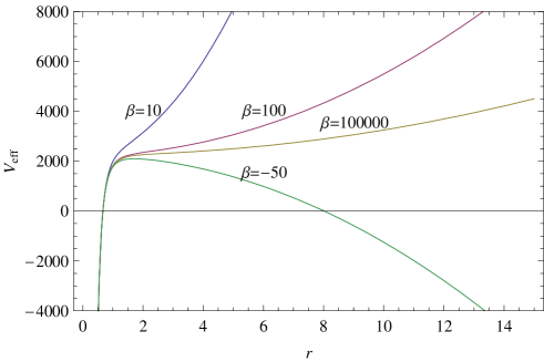
Figure 1: Variation of the effective potential with radial distance for different $\beta$ and $l=15$

In Figure 1 we have plotted the effective potential $V_{\rm eff}(r)$ against the radial coordinate $r$ choosing different values for the parameter $\beta$. One can readily notice from the plots that the effective potential is positive definite for all positive values of $\beta$ whereas for negative values of $\beta$ (with $l^{2}>|\beta|$) the potential has a sign-flip, as it goes again below the demarkation line zero. As in gpdsch we can readily interpret this distinctive feature of the effective potential for negative $\beta$ as the outcome of a repulsive force acting on the particle. This will lead to interesting cosmological consequences, which will be revealed in due course. This is the main interest of the present work.

The new parameter $\mu$ has an interesting physical significance. To realize this, let us notice that the effective potential can be re-written as

$$V_{\rm eff}=F(r)\left(1+\frac{l^{2}}{r^{2}}\right)$$ (9)

with the induced radial function $F(r)$ defined as

$$F(r)=\left(k-\frac{2M}{r^{2}}+\Lambda_{5}r^{2}\right)\left(\frac{\mu^{2}r^{2}+l^{2}}{r^{2}+l^{2}}\right).$$ (10)

Incorporating the above redefinitions into the radial dynamics (6) leads to a situation analogous to a pure Schwarzschild-AdS space-time where the mass $m$ of a particle is modified as $m^{2}\rightarrow\mu^{2}m^{2}$. This modification of mass can be realized by observing that the mass-shell condition (5) can be written now in the form $p^{2}+m^{2}\mu^{2}=0$. Thus, one can say that a generalized particle dynamics in a Schwarzschild-AdS background is identical to a standard particle dynamics in the background of an asymptotically AdS space-time (with $m^{2}\rightarrow\mu^{2}m^{2}$) where the induced metric is of the form

$$ds^{2}_{4+1}=-F(r)dt^{2}+\frac{dr^{2}}{F(r)}+r^{2}d\Omega_{3}^{2}$$ (11)

considering $c=1$. For $\mu^{2}=1$, equation (11) reduces to the standard Schwarzschild-AdS metric. We shall make use of the effective metric (11) in deriving the possible cosmological consequences later on in this article.

III Kaluza-Klein interpretation

The non-minimal particle dynamics (3) referred to in the previous section can indeed be derived from a minimal model in a space-time with one more spatial dimension, by imposing a constraint on the additional momentum component $p_{d+1}=0$ and then performing Kaluza-Klein type decomposition. In this section we shall derive this result in details for arbitrary spacetime dimensions.

Let us consider a particle of mass $m$ performing geodesic motion in a ($d+1$)-dimensional space-time with metric $G_{AB}$ ($A,B=0,1,...,d)$. The dynamics is described by the action

$$S=m\int d\tau\left(\frac{1}{2e}\,G_{AB}\,\dot{x}^{A}\dot{x}^{B}-\frac{e}{2}\right)\simeq-m\int d\tau\sqrt{-G_{AB}\,\dot{x}^{A}\dot{x}^{B}},$$ (12)

where the second expression follows by eliminating $e$ by its equation of motion

$$e^{2}=-G_{AB}\,\dot{x}^{A}\dot{x}^{B}.$$ (13)

The canonical momenta corresponding to the above action are given by

$$p_{A}=\frac{m}{e}\,G_{AB}\,\dot{x}^{B}\simeq\frac{m\,G_{AB}\,\dot{x}^{B}}{\sqrt{-G_{MN}\dot{x}^{M}\dot{x}^{N}}}.$$ (14)

They satisfy the Hamiltonian constraint

$$\frac{2m}{e}\,H=G^{AB}p_{A}p_{B}+m^{2}=0.$$ (15)

The Hamiltonian equations of motion can be written as

$$\dot{x}^{A}=\left\{x^{A},H\right\}~{}~{}~{},~{}~{}~{}\dot{p}_{A}=\left\{p_{A},H\right\},$$ (16)

which readily gives the covariant equation

$$\dot{p}_{A}-\dot{x}^{B}\,\Gamma_{BA}^{\;\;\;C}\,p_{C}=0.$$ (17)

We know that if the space-time geometry possesses isometries, there exist Killing vectors $\xi^{A}$ which satisfy the relation

$$D_{A}\xi_{B}+D_{B}\xi_{A}=0.$$ (18)

Then one can construct constants of motion of the following form

$$C[\xi]=\xi^{A}p_{A}~{}~{}~{},~{}~{}~{}\Rightarrow~{}~{}\dot{C}[\xi]=0.$$ (19)

Employing Kaluza-Klein decomposition, let us now consider a special form for the space-time with metric

$$G_{AB}=\left(\begin{array}[]{cc}g_{\mu\nu}&-n_{\mu}\\ -n_{\nu}&n^{2}+\beta\\ \end{array}\right)~{}~{}~{},~{}~{}~{}(\mu,\nu)=(0,1,...,d-1)$$ (20)

where $g_{\mu\nu}$ is the metric for the $d$-dimensional subspace, $n_{\mu}=g_{\mu\nu}n^{\nu}$ the normal vectors, and $n^{2}=g_{\mu\nu}n^{\mu}n^{\nu}$. Also, $\beta$ is just a numerical constant which takes care of the consistency of the theory. Then the inverse metric takes the form

$$G^{AB}=\left(\begin{array}[]{cc}g^{\mu\nu}+\frac{1}{\beta}n^{\mu}n^{\nu}&\frac{1}{\beta}\,n^{\mu}\\ \frac{1}{\beta}\,n^{\nu}&\frac{1}{\beta}\\ \end{array}\right)$$ (21)

where $g^{\mu\nu}$ is the usual $d$-dimensional inverse of $g_{\mu\nu}$. We further specialize to the case where all components are independent of $x^{d}$, implying

$$G_{AB,d}=0~{}~{}\Rightarrow~{}~{}g_{\mu\nu,d}=0~{}~{},~{}~{}n_{\mu,d}=0.$$ (22)

Consequently, $g_{\mu\nu}$ depends only on the co-ordinates $x^{\mu}$ and is the universal metric on all $d$-dimensional subspaces $x^{d}=$ constant. Technically speaking,

$$dx^{d}=0~{}~{}~{}\Rightarrow~{}~{}~{}G_{AB}dx^{A}dx^{B}=g_{\mu\nu}dx^{\mu}dx^{\nu}.$$ (23)

It follows that there is translation invariance in the $x^{d}$ direction, generated by the Killing vector $\xi^{A}_{(d)}=(0,...,0,1)$, and the momentum component in the $x^{d}$-direction is conserved. Hence

$$\dot{p}_{d}=0~{}~{}~{}\Rightarrow~{}~{}~{}\xi^{A}_{(d)}\,p_{A}=p_{d}=\mbox{constant}.$$ (24)

which can be shown explicitly using the equation of motion. Finally, we assume the $d$-dimensional subspace to have an internal isometry generated by a $d$-dimensional Killing vector $\xi^{\mu}$. Then we can specify the off-diagonal metric components to be given by the covariant components of this Killing vector: $n_{\mu}=\xi_{\mu}$, which implies

$$n_{\mu;\nu}+n_{\nu;\mu}=\xi_{\mu;\nu}+\xi_{\nu;\mu}=0,$$ (25)

where the semicolon denotes a $d$-dimensional covariant derivative. Defining the relation

$$\frac{1}{e}\,\dot{x}^{d}=\lambda$$ (26)

the action (12) reduces to

$$S=m\int d\tau\left[\frac{1}{2e}\,g_{\mu\nu}\,\dot{x}^{\mu}\dot{x}^{\nu}-\frac{e}{2}-\lambda\xi\cdot\dot{x}+\frac{e}{2}\lambda^{2}\left(\xi^{2}+\beta\right)\right],$$ (27)

which is precisely the action of generalized particle dynamics proposed in Eq (1). Note that taking $\lambda$ as a fundamental variable rather than $x^{d}$ does change the Euler-Lagrange equations of motion, as we loose a time-derivative. The net effect is, however, to constrain the $d$-component of the momentum to vanish:

$$p_{d}=0,$$ (28)

which is a particular solution of eq. (24). Indeed, one can conclude this by inserting the explicit expression for $p_{d}$ and using the Euler-Lagrange equation of motion for $\lambda$.

Finally we observe, that a Killing vector $\xi^{\mu}$ of the $d$-dimensional subspace can be lifted to a Killing vector of the full $(d+1)$-dimensional space-time by taking

$$\xi_{A}=(0,...,0,\beta)~{}~{}~{}\Leftrightarrow~{}~{}~{}\xi^{A}=(\xi^{\mu},1).$$ (29)

In this model, as all affine connection components $\Gamma_{AB}^{\;\;\;\;d}=0$ and $\beta$ is a constant, it follows immediately that eq. (18) is satisfied.

We thus arrive at the following significant conclusion: The generalized particle dynamics in $d$-dimensional space-time is equivalent to a special class of geodesic motions in a $(d+1)$-dimensional space-time with metric (20), which is an outcome of Kaluza-Klein decomposition, with $n_{\mu}=\xi_{\mu}$, and characterized by $p_{d}=0$.

IV Modeling Dark Energy

Having convinced that the choice of radial function (11) in the framework of generalized particle dynamics (1) can be obtained through Kaluza-Klein decomposition technique, we now turn to its cosmological implications. In order to obtain cosmologically relevant conclusions, both from theoretical and observational ground, we need to formulate a cosmological model and estimate physically observable quantities in $(3+1)$-dimensions. This is done by embedding a $(3+1)$-dimensional FLRW space-time into the $(4+1)$-dimensional effective metric (11) and find out its consequences (for details of the formalism, see (brde ; bwg )). Thus, as the observable universe is $(3+1)$-dimensional, we ultimately land up with a $(3+1)$-dimensional cosmological scenario embedded in a $(4+1)$-dimensional background. That is why we chose the background spacetime to be $(4+1)$-dimensional as our starting point.

The $(3+1)$-dimensional FLRW metric in terms of the coordinates $(T,\sigma,\theta,\varphi)$ is

$$ds_{3+1}^{2}=-dT^{2}+a(T)^{2}\left[\frac{d\sigma^{2}}{1-k\sigma^{2}}+\sigma^{2}(d\theta^{2}+\sin^{2}\theta\,d\varphi^{2})\right],$$ (30)

Friedmann equation in a cosmological model with cosmological constant $\Lambda$ is given by:

$$\frac{\dot{a}^{2}}{a^{2}}=-\frac{k}{a^{2}}+\frac{\Lambda}{3}+\frac{8\pi G_{3+1}\rho}{3}.$$ (31)

For embedding in the brane world scenario, we exploit the well-known embedding mechanism with the Gauss-Codazzi junction conditions and $Z_{2}$ symmetry gpdsch ; bwg and incorporate the usual practice of identifying $r(T)$ with $a(T)$. Some comments regarding the application of Gauss-Codazzi conditions in the present context is discussed in Section V. Using these junction conditions and $Z_{2}$ symmetry, we then arrive at the modified Friedmann equation for our model, with spatially flat universe (k=0), consistent with energy-conservation of ordinary matter on the brane, as

$$\frac{\dot{a}^{2}}{a^{2}}=-\frac{F(a)}{a^{2}}+\left(\frac{8\pi G_{4+1}\rho_{3+1}}{3}\right)^{2}.$$ (32)

Using the decomposition $\rho_{3+1}=\rho_{0}+\rho$, where $\rho$ is the ordinary matter density on the brane and $\rho_{0}$ is the brane tension, the modified Friedmann equation (32) now becomes:

$$\frac{\dot{a}^{2}}{a^{2}}=-\frac{F(a)}{a^{2}}+\left(\frac{8\pi G_{3+1}}{3}\right)\left[\frac{1}{2}\rho_{0}+\rho+\frac{1}{2}\frac{\rho^{2}}{\rho_{0}}\right],$$ (33)

where

$$G_{3+1}=\left(\frac{16\pi G_{4+1}^{2}\rho_{0}}{3}\right).$$

For confinement of matter on the brane (so that the brane matter does not escape into the bulk freely), the brane tension $\rho_{0}$ is considered to be much larger than $\rho$, i.e. $\rho_{0}\gg\rho$. Hence the $\rho^{2}$ term in the Friedmann equation (33) is suppressed. Then the final form of the modified Friedmann equation (33) is:

$$\frac{\dot{a}^{2}}{a^{2}}=-\frac{F(a)}{a^{2}}+\frac{4\pi G_{3+1}\rho_{0}}{3}+\frac{8\pi G_{3+1}\rho}{3}.$$ (34)

This modified Friedmann equation (34) is then compared with the normal Friedmann equation (31) for further study in cosmology.
For our model, this $F(a)$ in (34) is the radial function (10) of the induced Schwarzschild-AdS metric (11) and hence in our case, the modified Friedmann equations turns out to be

$$\left(\frac{\dot{a}}{a}\right)^{2}=\frac{8\pi G_{3+1}}{3}\rho+\frac{2M}{a^{4}}+\left[\alpha-\Lambda_{5}+\frac{l^{2}(2M/a^{2}-\Lambda_{5}a^{2})}{\beta(a^{2}+l^{2})}\right]$$ (35)

$$\frac{\ddot{a}}{a}=-\frac{4\pi G_{3+1}}{3}(\rho+3p)-\frac{2M}{a^{4}}+\left[\alpha-\Lambda_{5}-\frac{l^{2}(\Lambda_{5}a^{4}+2M+2\Lambda_{5}l^{2}a^{2})}{\beta(a^{2}+l^{2})^{2}}\right]$$ (36)

where $\dot{a}=da/dT$ and $\alpha=\left(8\pi G_{4+1}\rho_{0}/3\right)^{2}$. Identifying this equation (35) with (34), it becomes clear that except the first term $\frac{8\pi G_{3+1}}{3}\rho$, which is also present in normal Friedmann equation (31), all other terms in the r.h.s. of (35) are originated either from $F(a)$ or the brane tension $\rho_{0}$ of the modified Friedmann equation (34). So these terms are geometrical ((4+1)-dimensional geometry) in nature. Thus, for our cosmological model, only the knowledge about the bulk geometry is important. Once somehow the bulk geometry is known (as is the case in our model), the bulk source term ((4+1)-dimensional energy-momentum tensor) becomes irrelevant for the field equations on the brane (Einstein equation for brane) since there is no energy-momentum (matter) exchange between the brane and the bulk.
The terms containing $M$ ($\propto a^{-4}$) in (35, 36) contribute to the radiation energy density of the universe (constrained by Nucleosynthesis data to contribute to $\leq.03\%$ of total radiation energy density bwg ). We express the Hubble parameter $H=\dot{a}/a$ in terms of the redshift $z$ (where $1+z=a_{0}/a=1/a$) and neglect contributions from any cosmic constituent which redshifts away at the rate of radiation or faster (order of $(1+z)^{4}$ or higher) for a late time universe, to express the Friedmann equation (35) in a convenient form:

$$H^{2}=H_{0}^{2}\left[\Omega_{X}\left(1+b(1+z)^{2}\right)+\Omega_{M}(1+z)^{3}\right]$$ (37)

where $\Omega_{M}(1+z)^{3}=8\pi G_{3+1}\rho/3H_{0}^{2}$ and $\Omega_{X}=(\alpha-\Lambda_{5}\mu^{2})/H_{0}^{2}$ denote respectively the density parameters for the matter sector and for the additional terms coming from our modified gravity theory, with the dimensionless parameter $b=\Lambda_{5}\beta(\mu^{2}-1)^{2}/(\alpha-\Lambda_{5}\mu^{2})$. Observations fix $H_{0}=70.5\pm 1.3~{}{\rm km/s/Mpc}$ from the WMAP5 data wmap5 and $H_{0}=74.2\pm 3.6~{}{\rm km/s/Mpc}$ from the SHOES Team data shoes . Eq. (37) is the major result of our letter, the implications of which we analyze below.

Physical implications of the parameters are as follows: $\Omega_{M}$, the sum-total of the density-fraction for luminous and dark matter contributes $0.28\pm 0.08$ of total cosmic density, as fixed independently by the CMB hstcmb and large scale structure data lsst . Hence, for a valid dark energy model, $\Omega_{X}$ accounts for the DE density. However, observations indicate a universe close to the $\Lambda$CDM model. This forces $b$ to be small and $\beta$ large ($\mu$ contains $\beta$ in the denominator). Observationally, these values will be restricted by $\chi^{2}$ fitting, which we discuss later.

A crucial part from observational ground is to develop and estimate the observable parameters to show that we have a late accelerating universe where $\Omega_{X}$ accounts for the dark energy density. We show that, consistent with observations, our candidate dark energy EOS $(w_{X})$ indeed crosses the phantom divider.

Luminosity-redshift relation: This determines dark energy density $\Omega_{X}$ from observations, and, for our model (37), is given by

$$d_{L}(z)=(1+z)\int_{0}^{z}\frac{dz^{\prime}}{H(z^{\prime})}=\frac{(1+z)}{H_{0}}\int_{0}^{z}\frac{dz^{\prime}}{\left[\Omega_{X}\left(1+b(1+z^{\prime})^{2}\right)+\Omega_{M}(1+z^{\prime})^{3}\right]^{1/2}}.$$ (38)

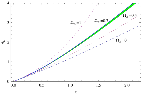
Figure 2: Variation of the luminosity distance with redshift for different $\Omega_{X}$

In Figure 2 the variation of $d_{L}$ with redshift in units of $H_{0}^{-1}$ for different $\Omega_{X}$ (with $\Omega_{M}+\Omega_{X}=1$) is shown using numerical integration. The plots show that a universe with $\Omega_{X}\sim 0.7,~{}\Omega_{M}\sim 0.3$ is favored in this model, and confirms that $\Omega_{X}$ accounts for the dark energy density. The allowed region (dark shade) gives the bound for $b$ as $-0.07\leq b<0$. Throughout the rest of the paper, we take a representative small negative value for $b=-0.05$. Once the luminosity distance is estimated, the apparent magnitude of the Supernovae can be calculated from the Hubble constant-free distance modulus de $\mu(z)=5\log_{10}\left[d_{L}(z)/{\rm Mpc}\right]+25$. With $d_{L}$ in Eq. (38), we have checked that the plot for this quantity too matches observations.

Age of the universe: It has the currently accepted value of $13.7\pm 0.02$ Gyr hstcmb and (up to a certain redshift $z$), is expressed as

$$t(z)=\int_{z}^{\infty}\frac{dz^{\prime}}{(1+z^{\prime})H(z^{\prime})}=\frac{1}{H_{0}}\int_{z}^{\infty}\frac{dz^{\prime}}{(1+z^{\prime})\left[\Omega_{X}\left(1+b(1+z^{\prime})^{2}\right)+\Omega_{M}(1+z^{\prime})^{3}\right]^{1/2}}.$$ (39)

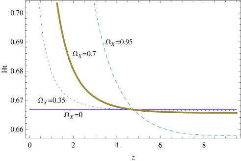
Figure 3: Variation of H(z)t(z) with z in units of $H_{0}^{-1}$

In Figure 3 we numerically plot $H(z)t(z)$ against redshift, showing that $\Omega_{X}\sim 0.7$ represents the most acceptable behavior.

Deceleration parameter: This will explicitly show the late accelerating behavior. From (37) we have

$$q(z)=\frac{-\ddot{a}/a}{\dot{a}^{2}/a^{2}}=\frac{H^{\prime}(z)}{H(z)}(1+z)-1=\frac{\Omega_{M}(1+z)^{3}-2\Omega_{X}}{2(\Omega_{X}(1+b(1+z)^{2})+\Omega_{M}(1+z)^{3})}.$$ (40)

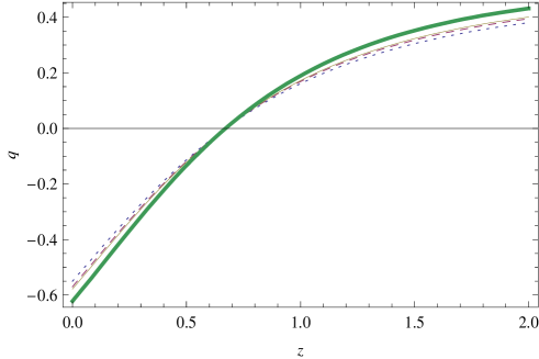
Figure 4: Variation of the deceleration parameter $q$ with redshift $z$ for different values of $b$. The dotted, dashed, thin and thick lines correspond respectively to the values $b=0,-.05,-.07,-.165$.

In Figure 4, the deceleration parameter has been plotted against redshift for $\Omega_{X}\sim 0.7,\Omega_{M}\sim 0.3$ with different values of $b$. The plots confirm that our model indeed results in an early decelerating and late accelerating universe. Moreover, onset of the recent accelerating phase, when the universe was $\sim 60\%$ of its present size ($z=0.6$), is also confirmed by our model.

Equation of state (EOS): The effective EOS of DE in our model is

$$w_{X}(z)=\frac{2q(z)-1}{3[1-\Omega_{M}(z)]}=-1+\frac{2b(1+z)^{2}}{3}.$$ (41)

The expression has been obtained by a binomial expansion considering small $b$ and dropping terms of order $(1+z)^{4}$ or higher, as before. Obviously, since $b$ is negative and non-zero, the effective EOS of dark energy candidate satisfies $w_{X}<-1$. So it shows a phantom like behavior that is as claimed by SN1a Gold data set pdlobs .

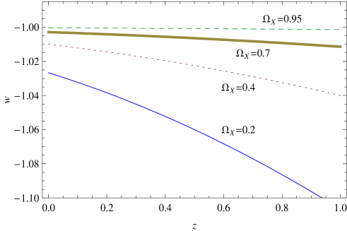
Figure 5: Variation of the effective EOS of dark energy with redshift

In Figure 5, the effective EOS parameter of dark energy with redshift is shown for different values of $\Omega_{X}$. The latest WMAP5 data constrains the lower bound of the dark energy EOS today to be $-1.11<w_{DE}$ wmap5 . This sets the lower bound of $b$ at $(-.165\leq b)$, which is way below its lower bound $(-.07\leq b)$ as predicted before from the luminosity-redshift relation. This model with $(-.07\leq b<0)$ will thus fit well with a more precise bound for the EOS available in the future.

Statefinder parameters $\{r,s\}$: The parameters statefinder

$$r=\frac{\dddot{a}/a}{(\dot{a}/a)^{3}}=1+\left[\frac{H^{\prime\prime}}{H}+\left(\frac{H^{\prime}}{H}\right)^{2}\right](1+z)^{2}-2\frac{H^{\prime}}{H}(1+z)~{};~{}s=\frac{2}{3}\frac{r-1}{2q-1}$$ (42)

can distinguish dynamical models from $\Lambda$CDM. In our model, $\{r,s\}$ pair is

$$r=1-\frac{b\Omega_{X}(1+z)^{2}}{\Omega_{X}(1+b(1+z)^{2})+\Omega_{M}(1+z)^{3}}~{};~{}s=\frac{2}{3}\frac{b(1+z)^{2}}{\left[3+b(1+z)^{2}\right]}$$ (43)

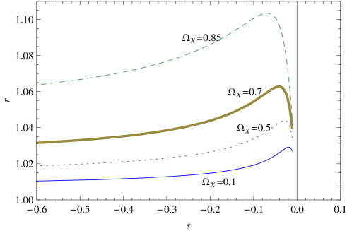
Figure 6: Variation of r with s

In figure 6 we plot $r$ versus $s$. The one with $\Omega_{X}=0.7$ is the most favored plot in our model. Hence, in so far as $b$ is non-trivial (as in the present case), the $\{r,s\}$ pair can distinguish our alternative gravity model from $\Lambda$CDM (for which $r=1,s=0$).

V Summary and outlook

Let us summarize. We have constructed a specific modified gravity structure, induced by a higher dimensional non-minimal particle dynamics framework. This particular generalized relativistic particle model was introduced by us in gpdsch . Subsequently we consider brane models embedded in this modified (4+1)-dimensional AdS-Schwarzschild spacetime. Note that we are dealing with an effective theory of gravity and its applications to cosmology, since derivation of our induced (4+1)-dimensional metric, generated by an yet unknown source term, remain an open issue. Indeed, to project the DE feature, it is bound to be of a novel nature. Furthermore, this issue is closely related to the use of Gauss-Codazzi equations in Section IV, which requires the metric to be a solution of Einstein’s equation. Our analysis in section III, in the Kaluza-Klein framework indicates that it is reasonable to expect our effective metric to be compatible with Einstein’s equation with a suitable source term.
The most promising feature of our work lies in the fact that the induced particle dynamics can simulate cosmological evolution with a late time accelerating universe. Not only that; in our formulation, it is also possible to have an effective phantom dark energy model without invoking the phantom. This is (quantitatively) manifested in the crossover of the phantom barrier. Our model is qualitatively distinct, but not quantitatively far off, from the $\Lambda$CDM model during recent times. Hence all the positive features of $\Lambda$CDM along with a phantom behavior (without the problems related to the negative kinetic term) can be accommodated in our model.
Several aspects of the proposed framework can be investigated further. The parameters used in the model can be constrained observationally by using a maximum likelihood method involving the minimization of the function $\chi^{2}=\sum_{1=1}^{N}\left[d_{L}(z)_{\rm obs}-d_{L}(z)_{\rm th}\right]^{2}/\sigma_{i}^{2}$, where $d_{L}(z)_{\rm th}$ contains the parameters used in a specific theory, $N$ is the number of Supernovae (taken as 157 for the most reliable Gold dataset) and $\sigma_{i}$ are the $1\sigma$ errors from the observational method used de . Observationally, this is the most accurate probe of $\Omega_{\rm DE}$; it will further constrain the parameters used in our model. Further, the variable EOS may be reflected in the Integrated Sachs-Wolfe (ISW) effect, which will serve as another test for the model. Studying features related to perturbations in this cosmological framework is another open issue.

References

- (1) S. Perlmutter et al., Astrophys. J. 517 (1999) 565; A. Riess et al., Astrophys. J. 116, 1009 (1998); P. Astier et. al., Astron. Astrophys. 447 (2006) 31.
- (2) W. L. Freedman et al., Astrophys. J. 553 (2001) 47; D. N. Spergel et al., Astrophys. J. 148 (2003) 175; ibid, Astrophys. J. Suppl. 170, 377 (2007).
- (3) E. Komatsu et. al., Astrophys. J. Suppl. 180, 330 (2009)
- (4) A. Riess et al., Astrophys. J. 699, 539 (2009) [arXiv:0905.0695]
- (5) R. R. Cadwell, Phys. Lett. B 545, 23 (2002)
- (6) S. M. Carroll, Living Rev. Relativity 3 (2001) 1; T. Padmanabhan, Phys. Rept. 380, 235 (2003); E. J. Copeland, M. Sami and S. Tsujikawa, Int. J. Mod. Phys. D 15, 1753 (2006); J. Frieman, M. Turner and D. Huterer, Ann. Rev. Astron. Astrophys. 46, 385 (2008); A. Silvestri and M. Trodden, arXiv:0904.0024
- (7) S. Nesseris and L. Perivolaropoulos, Phys. Rev. D70 (2004) 043531; ibid D72 (2005) 123519; J. Kujat, R. J. Scherrer and A. A. Sen, Phys. Rev. D74 (2006) 083501; S. Sur and S. Das, JCAP 0901 (2009) 007; C. G. Boehmer and J. Burnett, arXiv:0906.1351
- (8) L. Perivolaropoulos, JCAP 0510 (2005) 001; R. Gannouji, D. Polarski, A. Ranquet and A. A. Starobinsky, JCAP 0609, 016 (2006); L. P. Chimento, R. Lazkoz, R. Maartens and I. Quiros, JCAP 0609 (2006) 004; S. Nesseris and L. Perivolaropoulos, JCAP 0701, 018 (2007); S-F. Wu, A. Chatrabhuti, G-H. Yang and P-M. Zhang, Phys. Lett. B659, 45 (2008); H. Garcia-Compean, G. Garcia-Jimenez, O. Obregon and C. Ramirez, JCAP 0807, 016 (2008)
- (9) R. A. Brown, R. Maartens, E. Papantonopoulos and V. Zamarias, JCAP 11 (2005) 008; V. Sahni and Y. Shtanov, JCAP 11 (2003) 014; Y. Shtanov, A. Viznyuk and V. Sahni, Class. Quant. Grav. 24 (2007) 6159; Y. Shtanov, V. Sahni, A. Shafieloo and A. Toporensky, JCAP 0904 (2009) 023
- (10) S. Das, S. Ghosh, J. W. van Holten and S. Pal, JHEP 0904 (2009) 115 [arXiv:0902.2304]
- (11) R. Maartens, Living Rev. Relativity 7 (2004) 7; C. Barcelo and M. Visser, Phys. Lett. B 482, 183 (2000); J. Garriga and M. Sasaki, Phys. Rev. D62 (2000) 043523; S. Mukohyama, T. Shiromizu and K. Maeda, Phys. Rev. D 62, 024028 (2000); P. Bowcock, C. Charmousis and R. Gregory, Class. Quant. Grav. 17, 4745 (2000); S. Pal, Phys. Rev. D 74, 024005 (2006); ibid D 78, 043517 (2008)
- (12) Lisa Randall, Raman Sundrum, Phys. Rev. Lett. 83:3370 1999 (arXiv:hep-ph/9905221); Phys.Rev.Lett.83:4690,1999 (arXiv:hep-th/9906064)
- (13) For AdS-CFT correspondence, see for example M.Rangamani, Class.Quant.Grav.26:224003,2009 (arXiv:0905.4352)
- (14) J.W. van Holten, Phys.Rev.D75 (2007) 025027 (hep-th/0612216); R.H. Rietdijk and J.W. van Holten, Nucl.Phys.B472 (1996) 427 (hep-th/9511166); R.H. Rietdijk and J.W. van Holten, Nucl.Phys.B404 (1993) 42,.(hep-th/9303112); J.W. van Holten and R.H. Rietdijk, J.Geom.Phys.11:559,1993 (hep-th/9205074)
- (15) L. Verde et.al., Mon. Not. Roy. Astron. Soc. 335, 432 (2002)
- (16) V. Sahni, T. D. Saini, A. A. Starobinsky and U. Alam, JETP Lett. 77 (2003) 201; U. Alam, V. Sahni, T. D. Saini and A. A. Starobinsky, Mon. Not. Roy. Astron. Soc. 344 (2003) 1057