Quantum Hall Systems Studied by the Density Matrix
Renormalization Group Method

Abstract

The ground-state and low-energy excitations of quantum Hall systems are studied by the density matrix renormalization group (DMRG) method. From the ground-state pair correlation functions and low-energy excitions, the ground-state phase diagram is determined, which consists of incompressible liquid states, Fermi liquid type compressible liquid states, and many kinds of CDW states called stripe, bubble and Wigner crystal. The spin transition and the domain formation are studied at $\nu=2/3$. The evolution from composite fermion liquid state to an excitonic state in bilayer systems is investigated at total filling factor $\nu=1$.

1 Introduction

In two dimensional systems, applying perpendicular magnetic field strongly modifies the wave function of electrons leading to many interesting phenomena at low temperatures. The fractional quantum Hall effects[1] are typical example, where incompressible ground states are realized only at some fractional fillings of Landau levels.[2, 3] Since fractional quantum Hall effects are observed only in high quality samples, the Coulomb interaction between the electrons is thought to be essential rather than random potentials from impurities. This is contrasted with the case of integer quantum Hall effect where random potentials are essential. The importance of the Coulomb interaction in high magnetic field is followed from the increase in the energy scale of the Coulomb interaction. The wave function is scaled by the magnetic length $\ell=\sqrt{\hbar/eB}$, which is equivalent to the classical cyclotron radius $r_{c}$ in the lowest Landau level. The increase in the magnetic field decreases the magnetic length and enhances the energy scale of the Coulomb interaction between the electrons, $e^{2}/\varepsilon\ell$.

At typical magnetic field of 10T, $\ell$ is about 8nm, which is still much larger than the atomic length of 0.1nm. Since the conduction electrons are on the positive background charge from ions over length scale of $\ell$, the positive charge may be simplified to be uniform. Then the system is equivalent to the electron gas in a magnetic field, and $\ell$ becomes unique length scale of the system.

In the magnetic field, the kinetic energy is scaled by the cyclotron frequency $\omega_{c}=eB/m$, which is determined by the magnetic field $B$. The quantization of the wave function discretizes the classical cyclotron radius $r_{c}$, which also discretizes the kinetic energy and makes Landau levels $E=\hbar\omega_{c}(n+1/2)$. This means that the macroscopic number of electrons have the same energy in each Landau level, and large-scale degeneracy appears in the ground state. This macroscopic degeneracy is lifted by the Coulomb interaction between the electrons and various types of liquid states[4, 5, 6, 7, 8] and CDW states[9, 10, 11, 12] are realized depending on the filling of the Landau levels.

Since the ground state has macroscopic degeneracy in the limit of weak Coulomb interaction, standard perturbation theories are not useful. Thus numerical diagonalizations of the many body Hamiltonian have been used to study this system. Since numerical representation of the Hamiltonian needs complete set of many body basis states, we divide the system into unit cells with finite number of electrons in each cell. The properties of the infinite system are obtained by the finite size scalings. However, the number of many body basis states increases exponentially with the number of electrons. For example, when we study the ground state at $\nu=1/3$ with 18 electrons, each unit cell has 54 degenerated orbitals. The number of many body basis states is given by the combination of occupied and unoccupied orbitals, ${}_{54}C_{18}\sim 10^{14}$, which is practically impossible to manage by using standard numerical method such as exact diagonalization.

To study systems with typically more than 10 electrons, we need to reduce the number of many body basis states. For this purpose, we use the density matrix renormalization group (DMRG) method, which was originally developed by S. White in 1992.[13, 14] This method is a kind of variational method combined with a real space renormalization group method, which enables us to obtain the ground-state wave function of large-size systems with controlled high accuracy within a restricted number of many body basis states. The DMRG method has excellent features compared with other standard numerical methods. In contrast to the quantum Monte Carlo method, the DMRG method is free from statistical errors and the negative sign problem, which inhibit convergence of physical quantities at low temperatures. Compared with the exact diagonalization method, the DMRG method has no limitation in the size of system. The error in the DMRG calculation comes from restrictions of the number of basis states, which is systematically controlled by the density matrix calculated from the ground-state wave function, and the obtained results are easily improved by increasing the number of basis states retained in the system.

The application of the DMRG method to two-dimensional quantum systems is a challenging subject and many algorithms have been proposed. Most of them use mappings on to effective one-dimensional models with long-range interactions. However, the mapping from two-dimensional systems to one-dimensional effective models is not unique and proper mapping is necessary to keep high accuracy. In two-dimensional systems under a perpendicular magnetic field, all the one-particle wave functions $\Psi_{NX}(x,y)$ are identified by the Landau level index $N$ and the x-component of the guiding center, $X$, in Landau gage. The guiding center is essentially the center coordinate of the cyclotron motion of the electron and it is natural to use $X$ as a one-dimensional index of the effective model. More importantly, $X$ is discretized in finite unit cell of $L_{x}\times L_{y}$ through the relation to $y$-momentum, $X=k_{y}\ell^{2}$, which is discretized under the periodic boundary condition, $k_{y}=2\pi n/L_{y}$ with $n$ being an integer. Therefore, the two-dimensional continuous systems in magnetic field are naturally mapped on to effective one-dimensional lattice models, and we can apply the standard DMRG method.[15]

This method was first applied to interacting electron systems in a high Landau level and the ground-state phase diagram, which consists of various CDW states called stripe, bubble and Wigner crystal, has been determined.[16, 17] The ground state and low energy excitations in the lowest and the second lowest Landau levels have also been studied by the DMRG and the existence of various quantum liquid states such as Laughlin state and charge ordered states called Wigner crystal have been confirmed and new stripe state has been proposed.[18, 19]

In the following, we first explain the effective one-dimensional Hamiltonian used in the above studies and then show the results obtained for the spin polarized single layer system. We next review recent study on the spin transition and domain formation at $\nu=2/3$,[20] and finally explain the results on bilayer quantum Hall systems at $\nu=1$,[21] where crossover from a Fermi liquid state to an excitonic incompressible state occurs.

2 DMRG method

Here we briefly describe how the effective 1D Hamiltonian is obtained from 2D quantum Hall systems.[15] To describe the many body Hamiltonian for a interacting system, we first need to define one-particle basis states. Here, we use the eigenstates of free electrons in a magnetic field as one-particle basis states and represent the wave function $\Psi_{NX}(x,y)$ in Landau gauge:

$$\Psi_{NX}(x,y)=C_{N}\exp{\left[i{k_{y}y}-\frac{(x-X)^{2}}{2\ell^{2}}\right]}H_{N}\left[\frac{x-X}{\ell}\right],$$ (1)

where $H_{N}$ are Hermite polynomials and $C_{N}$ is the normalization constant. Then all the eigenstates $\Psi_{NX}(x,y)$ are specified using two independent parameters $N$ and $X$; $N$ is the Landau level index and $X$ is the $x$-component of the guiding center coordinates of the electron. Since the guiding center $X$ is related to the momentum $k_{y}$ as $X=k_{y}\ell^{2}$, and $k_{y}$ is discretized under the periodic boundary conditions, the guiding center $X$ takes only discrete values

$$X_{n}=2\pi\ell^{2}n/L_{y},$$ (2)

where $L_{y}$ is the length of the unit cell in the $y$-direction.

If we fix the Landau level index $N$, all the one-particle states are specified by one-dimensional discrete parameter $X_{n}$. Since many body basis states are product states of one-particle states, they are also described by the combinations of $X_{n}$ of electrons in the system. Thus the system can be mapped on to an effective one-dimensional lattice model.

The macroscopic degeneracy in the ground state of free electrons in partially filled Landau level is lifted by the Coulomb interaction

$$V(r)=\frac{e^{2}}{\epsilon r}.$$ (3)

The Coulomb interaction makes correlations between the electrons and stabilizes various types of ground states depending on the filling $\nu$ of Landau levels. When the magnetic field is strong enough so that the Landau level splitting is sufficiently large compared with the typical Coulomb interaction $e^{2}/(\epsilon\ell)$, the electrons in fully occupied Landau levels are inert and the ground state is determined only by the electrons in the top most partially filled Landau level.

The Hamiltonian is then written by

$$H=S\sum_{n}c_{n}^{\dagger}c_{n}+\frac{1}{2}\sum_{n_{1}}\sum_{n_{2}}\sum_{n_{3}}\sum_{n_{4}}A_{n_{1}n_{2}n_{3}n_{4}}c_{n_{1}}^{\dagger}c_{n_{2}}^{\dagger}c_{n_{3}}c_{n_{4}},$$ (4)

where we have imposed periodic boundary conditions in both $x$- and $y$-directions, and $S$ is the classical Coulomb energy of Wigner crystal with a rectangular unit cell of $L_{x}\times L_{y}$[22]. $c_{n}^{\dagger}$ is the creation operator of the electron represented by the wave function defined in equation (1) with $X=X_{n}$. $A_{n_{1}n_{2}n_{3}n_{4}}$ are the matrix elements of the Coulomb interaction defined by

$$A_{n_{1}n_{2}n_{3}n_{4}} = \delta^{\prime}_{n_{1}+n_{2},n_{3}+n_{4}}\frac{1}{L_{x}L_{y}}\sum_{\mib q}\delta^{\prime}_{n_{1}-n_{4},q_{y}L_{y}/2\pi}\frac{2\pi e^{2}}{\epsilon q}$$ (5)

$${\mbox{\hskip 14.22636pt}}\times\left[L_{N}(q^{2}\ell^{2}/2)\right]^{2}\exp{\left[-\frac{q^{2}\ell^{2}}{2}-i(n_{1}-n_{3})\frac{q_{x}L_{x}}{M}\right]},$$

where $L_{N}(x)$ are Laguerre polynomials with $N$ being the Landau level index[17]. $\delta_{n_{1},n_{2}}^{\prime}=1$ when $n_{1}=n_{2}(\mbox{mod}\ M)$ with $M$ being the number of one-particle states in the unit cell, which is given by the area of the unit cell $2\pi M\ell^{2}=L_{x}L_{y}$.

Figure 1: Schematic diagrams for (a) infinite system algorithm and (b) finite system algorithm of the DMRG method. $\bullet$ represents a one-particle orbital in a given Landau level. B_L and B_R are left and right blocks, respectively.

In order to obtain the ground-state wave function we apply the DMRG method.[15] As shown in Fig. 1 (a), we start from a small-size system consisting of only four one-particle orbitals whose indices $n$ are 1, 2, $M-1$, and $M$, and we calculate the ground-state wave function. We then construct the left block containing one-particle orbitals of $n=1$ and 2, and the right block containing $n=M-1$ and $M$ by using eigenvectors of the density matrices which are calculated from the ground-state wave function. We then add two one-particle orbitals $n=3$ and $M-2$ between the two blocks and repeat the above procedure until $M$ one-particle orbitals are included in the system. We then apply the finite system algorithm of the DMRG shown in Fig. 1 (b) to refine the ground-state wave function. After we have obtained the convergence, we calculate correlation functions to identify the ground state.

The ground-state pair correlation function $g({\mib r})$ in guiding center coordinates is defined by

$$g({\mib r})=\frac{L_{x}L_{y}}{N_{e}(N_{e}-1)}\langle\Psi|\sum_{i\neq j}\delta({\mib r-\mib R}_{i}+{\mib R}_{j})|\Psi\rangle,$$ (6)

where ${\mib R}_{i}$ is the guiding center coordinate of the $i$th electron, and it is calculated from the following equation

$$g({\mib r}) = \frac{1}{N_{e}(N_{e}-1)}\sum_{\mib q}\sum_{n_{1},n_{2},n_{3},n_{4}}\exp\left[i{\mib q\cdot\mib r}-\frac{q^{2}\ell^{2}}{2}-i(n_{1}-n_{3})\frac{q_{x}L_{x}}{M}\right]\times$$ (7)

$$\mbox{\hskip 99.58464pt}\delta^{\prime}_{n_{1}-n_{4},q_{y}L_{y}/2\pi}\langle\Psi|c_{n_{1}}^{\dagger}c_{n_{2}}^{\dagger}c_{n_{3}}c_{n_{4}}|\Psi\rangle,$$

where $\Psi$ is the ground state and $N_{e}$ is the total number of electrons.

Figure 2: Eigenvalues $w_{\alpha}$ of the density matrix for two-dimensional system of 54 orbitals with 18 electrons. Sum of $w_{\alpha}$ is equivalent to the norm of the ground-state wave function and normalized to be unity.

The accuracy of the results depends on the distribution of eigenvalues of the density matrix. A typical example of the eigenvalues of the density matrix for system of $M=54$ with $18$ electrons is shown in Fig. 2, which shows an exponential decrease of eigenvalues $w_{\alpha}$. In this case accuracy of $10^{-4}$ is obtained by keeping more than one hundred states in each block.

3 Single layer system

Figure 3: The lowest excitation gap at various $\nu$ in the lowest Landau level. Relatively large excitation gap is obtained at fractional fillings $\nu=n/(2n+1)$. The excitation gap is in units of $e^{2}/(\epsilon\ell)$.

Here we present diverse ground states obtained by the DMRG method applied to the single layer quantum Hall systems. In the limit of strong magnetic field, the electrons occupy only the lowest Landau level $N=0$. In this limit, fractional quantum Hall effect (FQHE) has been observed at various fractional fillings[3]. The FQHE state is characterized by incompressible liquid with a finite excitation gap[1].

These FQHE states are confirmed by the DMRG calculations, where relatively large excitation gaps are obtained at various fillings between $\nu=1/2$ and 3/10[18] as shown in Fig. 3. We clearly find large excitation gaps at fractional fillings $\nu=1/3,2/5,3/7,4/9$ and $5/11$, which correspond to primary series of the FQHE at $\nu=n/(2n+1)$. The pair correlation function at $\nu=1/3$ is presented in Fig. 4, which shows a circularly symmetric correlation consistent with the Laughlin’s wave function.[1]

In the limit of low filling $\nu\rightarrow 0$, mean separation between the electrons becomes much longer than the typical length-scale of the one-particle wave function. In this limit the quantum fluctuations are not important and electrons behave as classical point charges. The ground state is then expected to be the Wigner crystal. The formation of the Wigner crystal is also confirmed by the DMRG calculations at low fillings as shown in Fig. 5 (a). The $\nu$-dependence of the low energy spectrum shows that the first-order transition to Wigner crystal occurs at $\nu\sim 1/7$.[18]

With decreasing magnetic field, electrons occupy higher Landau levels. In high Landau levels, the one-particle wave function extends over space leading to effective long range exchange interactions between the electrons. The long range interaction stabilizes CDW ground states and various types of CDW states called stripe and bubble are predicted by Hartree-Fock theory.[9] These CDW states are confirmed by the DMRG calculations as shown in Figs. 5 (b) and (c), where two-electron bubble state and stripe state are obtained at $\nu=8/27$ and $3/7$, respectively, in the $N=2$ Landau level. Although the CDW structures are similar to those obtained in the Hartree-Fock calculations, the ground state energy and the phase diagram are significantly different[16]. The DMRG results are consistent with recent experiments[10], and the discrepancy is due to the quantum fluctuations neglected in the Hartree-Fock calculations.

The ground-state phase diagram obtained by the DMRG is shown in Fig. 6. In the lowest Landau level, we find many liquid states at fractional fillings and around $\nu=1/2$. Nevertheless, CDW states dominate over the whole range of filling in higher Landau levels. This difference in the ground state phase diagram comes from different effective interactions between the electrons. In the lowest Landau level, the one particle wave function is localized within the magnetic length $\ell$, that yields strong short-range repulsion between the electrons. Since quantum liquid states such as Laughlin state are stabilized by the strong short-range repulsion, liquid states are realized in the lowest Landau level. In higher Landau levels, however, the wave function extends over space with the increase in the classical cyclotron radius $r_{c}$. Thus the short-range repulsion is reduced and liquid states become unstable. As shown in Fig. 7 (a), the real space effective interaction between the electrons in higher Landau levels has a shoulder structure around the distance twice the classical cyclotron radius. This structure of effective interaction makes minimum in the Coulomb potential near the guiding center of the electron as shown in Fig. 7 (b) and stabilizes the clustering of electrons. This is the reason why stripe and bubble states are realized in higher Landau levels.[19]

Figure 4: Pair correlation function $g({\bf r})$ at $\nu=1/3$ in the lowest Landau level. The length is in units of $\ell$.

Figure 5: Pair correlation functions $g({\bf r})$ in guiding center coordinates. (a) Wigner crystal realized in an excited state at $\nu=1/6$ in the lowest Landau level. The number of electrons in the unit cell $N_{e}$ is 12. (b) Two-electron bubble state at $\nu=8/27$ in $N=2$ Landau level. $N_{e}=16$. (c) Stripe state at $\nu=3/7$ in $N=2$ Landau level. $N_{e}=18$.

Figure 6: The ground state phase diagram obtained by the DMRG method. $N$ is the Landau level index and $\nu_{N}$ in the filling factor of the $N$th Landau level.

Figure 7: (a) Effective interaction between the electrons in the $N$th Landau level. $R_{c}$ is the classical cyclotron radius. (b) Coulomb potential made by two electrons separated by $\Delta x$.

4 Spin transitions

In two dimensional systems, strong perpendicular magnetic field completely quenches the kinetic energy of electrons. Since the kinetic energy is independent of the spin polarization, the exchange Coulomb interaction easily aligns the electron spin. The ferromagnetic ground state at $\nu=1/q$ ($q$ odd) is thus realized even in the absence of the Zeeman splitting[23]. At the filling $\nu=2/3$ and $2/5$, however, the paramagnetic ground states compete with the ferromagnetic state, and the Zeeman splitting $\Delta_{z}=g\mu_{B}B$ induces a spin transition[24]. Such a spin transition in fractional quantum Hall states has been naively explained by the composite fermion theory.[25] The composite fermions are electrons coupled with even number of fluxes. These fluxes effectively reduces external magnetic field and the $\nu=p/(2p\pm 1)$ fractional quantum Hall effect (FQHE) state is mapped on to the $\nu^{\prime}=p$ integer QHE state of composite fermions. The spin transitions at $\nu=2/3$ and 2/5[26] correspond to the spin transition at $\nu=2$, where the Zeeman splitting corresponds to the effective Landau level separation, and the energy levels of the minority spin state in the lowest Landau level and the majority spin state in the second lowest Landau level coincide.

Extensive experimental[27, 28, 29, 30, 31, 32, 33, 34, 35] and theoretical [36, 37, 38, 39] studies have been made on this transition. Nevertheless, there is no clear theoretical consensus on this issue. This is due to the difficulties of studies in this system. A number of states possibly compete in energy, and large enough systems are needed to see non-uniform structures in the partially polarized states. Here we use the DMRG method[15], and study the spin transition and the spin structures in large system to clarify the nature of the spin transition at $\nu=2/3$.

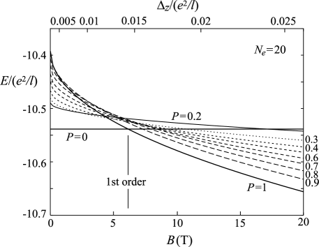
Figure 8: Lowest energies for fixed polarization ratio $P$ as a function of magnetic field $B$ at filling factor $\nu=2/3$ in units of $e^{2}/(\epsilon\ell)$. The total number of electron is 20. The aspect ratio is fixed at 2.0. The $g$-factor is 0.44.

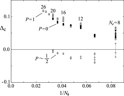
Figure 9: Charge gap of $\nu=2/3$ spin polarized states ($\Box$), unpolarized states ($\bullet$), and partially polarized states ($\circ$) for various $N_{e}$ and aspect ratios $L_{x}/L_{y}$. $\Delta_{c}$ is in units of $e^{2}/(\epsilon\ell)$.

We first calculate the energy at various polarization $P$ as a function of the Zeeman splitting, $\Delta_{z}=g\mu B$. The obtained results are shown in Fig. 8. In the absence of the Zeeman splitting, the unpolarized state ($P=0$) is the lowest. The energy of the polarized state ($P>0$) monotonically increases as $P$ increases. With the increase in Zeeman splitting $\Delta_{z}$, however, the energy of polarized state decreases and the fully polarized state ($P=1$) becomes the lowest. Figure 8 shows that the transition from the unpolarized state to the fully polarized state occurs at $B\simeq 6$T which is roughly consistent to the earlier work done in a spherical geometry. [24] In the present calculation on a torus, all partially polarized states ($0<P<1$) are higher in energy than the ground states ($P=0$ or 1). This feature is independent of the size of the system and the aspect ratio $L_{x}/L_{y}$, and indicates phase separations of $P=0$ and $P=1$ in partially polarized states.

The unpolarized state of $P=0$ and the fully polarized state of $P=1$ are both quantum Hall states with finite charge excitation gap, which is defined by

$$\Delta_{c}(P)=E(N_{\phi}+1,P)+E(N_{\phi}-1,P)-2E(N_{\phi},P),$$ (8)

where $N_{\phi}$ is the number of one-particle states in the lowest Landau level. The filling factor $\nu$ is then given by $N_{e}/N_{\phi}$. The charge gap $\Delta_{c}$ for various $N_{\phi}$ and aspect ratios of the unit cell is presented in Fig. 9. In this figure, the gap $\Delta_{c}$ seems to vanish for partially polarized state $P\sim 1/2$ in the limit of $N_{e}\rightarrow\infty$. This result clearly indicates that partially polarized state with $P\sim 1/2$ is a compressible state in contrast to the incompressible states at $P=0$ and $1$, where $\Delta_{c}$ remains to be finite in the limit of $N_{e}\rightarrow\infty$.

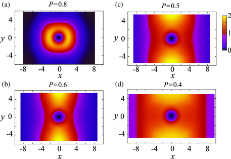
Figure 10: Pair correlation functions for minority spins $g_{\downarrow\downarrow}$ at $\nu=2/3$ for several polarization ratios (a) $P=0.8$, (b) $P=0.6$, (c) $P=0.5$, and (d) $P=0.4$.

To study the spin structure in the partially polarized states, we next calculate the pair-correlation function defined by

$$g_{\sigma\sigma}({\mib r})=\frac{L_{x}L_{y}}{N_{\sigma}(N_{\sigma}-1)}\langle\Psi|\sum_{nm}\delta({\mib r}+{\mib R}_{\sigma,n}-{\mib R}_{\sigma,m})|\Psi\rangle,$$ (9)

where $\sigma=\pm 1/2$ is the spin index and $N_{\sigma}$ is the number of electrons with spin $\sigma$. The spin structures in partially spin polarized states are clearly shown in the pair correlation function between minority spins. Namely, if unpolarized regions are formed in the partially polarized states, then electrons with minority spins are concentrated in the unpolarized regions. This concentration of the minority spins is shown in Fig. 10, which shows $g_{\downarrow\downarrow}(x,y)$ for partially polarized states at (a) $P=0.8$, (b) $P=0.6$, (c) $P=0.5$, and (d) $P=0.4$. When $P$ is close to $1$, for example $P=0.8$ shown in Fig. 10(a), a pair of minority spins is found only near the origin. As the polarization ratio $P$ decreases, minority spins make a domain around the origin, and two domain walls along the $y$-direction are formed. These domain walls move along $x$-direction and the domain of minority spin finally covers entire unit cell in the limit of $P=0$. This change in the size of the domain is consistent with the expectation that the domain in Fig. 10 corresponds to the unpolarized spin singlet region where the density of up-spin electrons and the down-spin electrons are the same.

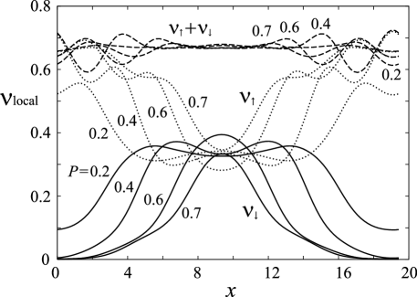
Figure 11: Local densities of up spin, and down spin electrons for various polarization ratios $P$ at $\nu=2/3$. The number of electrons is 20.

To confirm the separation of the unpolarized and polarized spin regions, we next consider the local electron density of up-spin electrons $\nu_{\uparrow}(x)$ and down-spin electrons $\nu_{\downarrow}(x)$. Figure 11 shows $\nu_{\uparrow}(x)$ and $\nu_{\downarrow}(x)$ for partially polarized states with $P=0.2,\ 0.4,\ 0.6$ and $0.7$. Here $\nu_{\uparrow}(x)$ and $\nu_{\downarrow}(x)$ are scaled to be the local filling factor of the lowest LL. Thus, the total local electron density $\nu_{\uparrow}(x)+\nu_{\downarrow}(x)$ is almost $2/3$. In this figure the separation to two regions is clearly seen; the unpolarized spin region around $L_{x}/2$, where both $\nu_{\uparrow}$ and $\nu_{\downarrow}$ are close to 1/3, and the fully polarized spin region around $x\sim 0$ or equivalently $x\sim L_{x}$, where $\nu_{\uparrow}$ is almost 2/3 while $\nu_{\downarrow}$ is close to 0. These results confirm the separation of the unpolarized and polarized spin regions as expected from the pair correlation functions shown in Fig. 11.

The polarized and unpolarized spin regions are separated by the domain walls whose width is about $4\ell$. This means that the phase separation is realized only for systems whose size of the unit cell $L_{x},(L_{y})$ is larger than twice the width of domain wall; $L_{x},(L_{y})>8\ell$. Indeed, exact diagonalization studies up to $N_{e}=8$ electrons have never found the phase separation at $\nu=2/3$.[39] We have found the phase separation only for large systems with $N_{e}>12$. We note that above behavior is generic over the aspect ratio. In an ideal system, the two states separate into two regions even when the system size is infinitely large. In experimental situations, however, multi-domain structures are realized due to the inhomogeneity and coupling with randomly distributed nuclear spins.

The DMRG study on the ground state energy for various polarization $P$ shows that the ground state at $\nu=2/3$ evolves discontinuously from the unpolarized $P=0$ state to the fully polarized $P=1$ state as the Zeeman splitting increases. In partially polarized states $0<P<1$, the electronic system separates spontaneously into two states; the $P=0$ and the $P=1$ states. These two states are separated by the domain wall of width $4\ell$. Since the energy of the domain wall is positive, the partially polarized states always have higher energy than that of $P=1$ or $P=0$ states. We think this is the reason of the direct first order transition from $P=0$ to $P=1$ state in the ground state.

It is useful to compare our result with the spin transition at $\nu=2$ which occurs when minority spin states in the lowest LL and majority spin states in the second lowest LL cross by varying the ratio of the Zeeman and Coulomb energy. The ground state at $\nu=2$ is thus a fully polarized state or a spin singlet state. In analogous to the case of $\nu=2/3$ the transition between them is first order[40], and spin domain walls have been found in high energy states.[41] This analogy can be expected, because the $\nu=2$ states and the $\nu=2/3$ states are connected in the composite fermion theory[25, 26], although the effective interaction between composite fermions is different from that for electrons.

5 Bilayer system

The properties of quantum Hall systems sensitively depend on the magnetic field, and various types of ground states including incompressible liquids[1], compressible liquids[42, 43], spin singlet liquid, CDW states called stripes, bubbles, and Wigner crystal are realized depending on the filling $\nu$ of Landau levels. In bilayer quantum Hall systems, additional length scale of the layer distance $d$, and the degrees of freedom of layers make the ground state much more diverse and interesting.[44]

Excitonic phase, namely Haplerin’s $\Psi_{1,1,1}$ state, is one of the ground states realized in bilayer quantum Hall systems at total filling $\nu=1$ at small layer separation $d$, where electrons and holes in different layers are bound with each other due to strong interlayer Coulomb interaction. This excitonic state has recently attracted much attention because a dramatic enhancement of zero bias tunneling conductance between the two layers[45], and the vanishing of the Hall counterflow resistance are observed[46, 47]. As the layer separation $d$ is increased, the excitonic phase vanishes, and at large enough separation, composite-fermion Fermi-liquid state is realized in each layer.

Several scenarios have been proposed for the transition of the ground state as the layer separation increases[48, 49, 50, 51, 52, 53, 54]. However how the excitonic state develops into independent Fermi-liquid state has not been fully understood. In this section we investigate the ground state of $\nu=1$ bilayer quantum Hall systems by using the DMRG method[15]. We calculate energy gap, two-particle correlation function $g(r)$ and excitonic correlation function for various values of layer separation $d$, and show the evolution of the ground state with increasing $d$.

The Hamiltonian of the bilayer quantum Hall systems is written by

$$H = \sum_{i<j}\sum_{\mib q}V(q)\ {\rm e}^{-q^{2}\ell^{2}/2}{\rm e}^{{\rm i}{\mib q}\cdot({\mib R}_{1,i}-{\mib R}_{1,j})}$$ (10)

$$+\sum_{i<j}\sum_{\mib q}V(q)\ {\rm e}^{-q^{2}\ell^{2}/2}{\rm e}^{{\rm i}{\mib q}\cdot({\mib R}_{2,i}-{\mib R}_{2,j})}$$

$$+\sum_{i,j}\sum_{\mib q}V(q)\ {\rm e}^{-qd}e^{-q^{2}\ell^{2}/2}{\rm e}^{{\rm i}{\mib q}\cdot({\mib R}_{1,i}-{\mib R}_{2,j})},$$

where ${\mib R}_{1,i}$ are the two-dimensional guiding center coordinates of the $i$th electron in the layer-1 and ${\mib R}_{2,i}$ are that in the layer-2. The guiding center coordinates satisfy the commutation relation, $[{R}_{j}^{x},{R}_{k}^{y}]={\rm i}\ell^{2}\delta_{jk}$. $V(q)=2\pi e^{2}/(\epsilon q)$ is the Fourier transform of the Coulomb interaction and the wave function is projected on to the lowest Landau level. We consider uniform positive background charge to cancel the component at $q=0$. We will assume zero interlayer tunneling and fully spin polarized ground state.

Figure 12: The exciton correlation of bilayer quantum Hall systems at $\nu=1$. The solid line represents $g_{\rm ex}(M/2)$. The dashed line represents $g_{\rm ex}(M/2-1)$.

In the limit of $d=0$, electrons in different layers can not occupy the same position because of the strong interlayer Coulomb repulsion. The strong interlayer repulsion makes electron-hole pairs, which is called excitons whose degrees of freedom are represented by interlayer dipoles or pseudo-spins at total filling $\nu=1$. The Coulomb exchange interaction aligns the interlayer dipoles (the pseudo-spins) leading to the macroscopic coherence of the excitons and Haplerin’s $\Psi_{1,1,1}$ state is realized.

To confirm the coherence of the excitons, we calculate the exciton correlation defined by

$$g_{\rm ex}(n)\equiv\frac{2M-1}{N_{1}N_{2}}\langle\Psi|c^{\dagger}_{1,n}c_{2,n}c^{\dagger}_{2,0}c_{1,0}|\Psi\rangle,$$ (11)

where $|\Psi\rangle$ is the ground state and $c^{\dagger}_{1,n}$ ($c^{\dagger}_{2,n}$) is the creation operator of the electrons in the $n$th one-particle state defined by

$$\phi_{n}({\mib r})=\frac{1}{\sqrt{L_{y}\pi^{1/2}\ell}}\exp\left\{ik_{y}y-\frac{(x-X_{n})^{2}}{2\ell^{2}}\right\}$$ (12)

in the layer-1 (layer-2). $X_{n}=nL_{x}/M=k_{y}\ell^{2}$ is the $x$-component of the guiding center coordinates and $L_{x}$ is the length of the unit cell in the $x$ direction. $M$ is the number of one-particle state in each layer. $N_{1}$ and $N_{2}$ are the number of electrons in the layer-1 and layer-2, respectively, and we impose the symmetric condition of $N_{1}=N_{2}$. Since $g_{\rm ex}(n)$ represents the correlations between the two excitons at $X=0$ and $X=X_{n}$, $\lim_{n\rightarrow\infty}g_{\rm ex}(n)\neq 0$ indicates existence of macroscopic coherence of excitons.

As is shown in Fig. 12, $g_{\rm ex}(n)$ tends to 1 as $d\to 0$, that confirms the macroscopic coherence of excitons at $d=0$. Indeed, Haplerin’s $\Psi_{1,1,1}$ state has the macroscopic coherence of excitons and $g_{\rm ex}(n)=1$ independent of $n$. In this figure we have shown $g_{\rm ex}(M/2)$ instead of $\lim_{n\rightarrow\infty}g_{\rm ex}(n)$, because the largest distance between the two excitons is $L_{x}/2$ in the finite unit cell of $L_{x}\times L_{y}$ under the periodic boundary conditions. In order to check the size effect, we also plot $g_{\rm ex}(M/2-1)$ with the dashed line. Since the difference between $g_{\rm ex}(M/2)$ and $g_{\rm ex}(M/2-1)$ is small, we expect $g_{\rm ex}(M/2)$ well represents the macroscopic coherence in the limit of $N\rightarrow\infty$. With increasing $d/\ell$, the excitonic correlation decreases monotonically and finally falls down to negligible value at $d/\ell\sim 1.6$.

Figure 13: The pseudo-spin excitation gap $\Delta_{ps}$ of bilayer quantum Hall systems at the total filling factor $\nu=1$. The dashed lines are guide for the eye.

The presence of macroscopic coherence of excitons shown in the Fig. 12 means the existence of ferromagnetic order of the interlayer dipoles (the pseudo-spins). Since interaction between the interlayer dipoles has SU(2) symmetry at $d=0$, corrective gapless excitations called pseudo-spin waves are expected. Even in the case of finite layer distance $d$, the Hamiltonian has continuous XY symmetry, and gapless pseudo-spin wave excitations are still expected. This is confirmed by the size dependence of the pseudo-spin excitation gap shown in Fig. 13, where the pseudo-spin excitation gap $\Delta_{ps}=E(N_{1}+1,N_{2}-1,M)-E(N_{1},N_{2},M)$ in finite system decreases as a function of $1/L_{x}$.

Figure 14: The charge excitation gap $\Delta_{c}$ of bilayer quantum Hall systems at the total filling factor $\nu=1$. The dashed lines are guide for the eye.

In contrast to the pseudo-spin excitation gap $\Delta_{ps}$, the charge excitation gap $\Delta_{c}$ defined by $\Delta_{c}=E(N_{1},N_{2},M-1)+E(N_{1},N_{2},M+1)-2E(N_{1},N_{2},M)$ seems to be finite even in the limit of $L_{x}\rightarrow\infty$ for small $d$ as shown in Fig. 14. The charge excitation brakes at least one electron-hole pair and it needs energy of order $V_{0}^{(1,2)}$ which is the pseudopotential between the electrons in different layers whose relative angular momentum is $0$. This pseudopotential decreases with the increase in the layer distance $d$, and thus the charge gap decreases with the increase in $d$.

We next see the lowest excitation gap in a fixed size of system. Figure 15 shows the result for $N_{e}=24$. The aspect ratio $L_{x}/L_{y}=1.8$ is chosen from the minimum of the ground state energy with respect to $L_{x}/L_{y}$ around $d/\ell=1.8$, where minimum structure appears in the ground state energy.

We can see clear excitation gap of finite system for $d/\ell<1.2$, where excitonic ground state is expected both theoretically and experimentally [45, 46, 47, 48, 49, 50, 51, 52, 53, 54]. The excitation gap rapidly decreases with increasing $d/\ell$ from $1.2$, and it becomes very small for $d/\ell>1.6$. This behavior is consistent with experiments.[55] Although the excitation gap for $d/\ell>1.7$ is not presented in the figure for $N_{e}=24$ because of the difficulty of the calculation of excited states in large system, we do not find any sign of level crossing in the ground state up to $d/\ell\sim 4$, where two layers are almost independent. These results suggest that the excitonic state at small $d/\ell$ continuously crossovers to compressible state at large $d/\ell$, that is consistent with the behaviors of exciton correlations $g_{\rm ex}(M/2)$ in Fig. 12, which shows $g_{\rm ex}(M/2)$ continuously approaches zero around $d/\ell\sim 1.6$. In the present calculation it is difficult to conclude whether the gap closes at finite $d/\ell\sim 1.6$ in the thermodynamic limit or excitonic state survives with exponentially small finite gap even for large $d/\ell>1.6$. We have calculated the excitation gap in different size of systems and aspect ratios, and obtained similar results as shown in the inset of Fig. 15.

Figure 15: The lowest excitation gap $\Delta$ of bilayer quantum Hall systems at the total filling factor $\nu=1$. $N_{e}=24$ and $L_{x}/L_{y}=1.6$. The inset shows the result for $N_{e}=18$ and $L_{x}/L_{y}=1.0$.

Concerning the first excited state, however, Fig. 15. shows a level crossing at $d/\ell\sim 1.2$, where we can see sudden decrease in the excitation gap. We expect that the lowest excitation at $d/\ell<1.2$ is the pseudo-spin excitation whose energy gap decreases with the increase in the size of system and tends to zero in the limit of large system. On the other hand, the lowest excitation at $d/\ell>1.2$ shown in Fig. 15 is expected to be the excitation to the roton minimum which corresponds to the bound state of quasiparticle and quasihole excitatins, whose energy increases with the decrease in $d/\ell$. This change in the character of the low energy excitations at $d/\ell\sim 1.2$ will be confirmed in a clear change in correlation functions in the excited state as shown later. We note that the position of the level crossing in the first excited state itself depends on the size of system because the pseudo-spin excitation gap decreases with the increase in the system size. However, the change in the character of the low energy excitations of finite systems is expected to remain even in the limit of large system, since the spectrum weight of pseudo-spin waves transfers to high energy with the increase in $d$.

We next calculate pair correlation functions of the electrons to see detailed evolution of the ground-state wave function. The interlayer pair correlation functions are defined by

$$g_{12}({\mib r}) \equiv \frac{L_{x}L_{y}}{N_{1}N_{2}}\langle\Psi|\sum_{n\ m}\delta({\mib r}+{\mib R}_{1,n}-{\mib R}_{2,m})|\Psi\rangle,$$ (13)

where $|\Psi\rangle$ is the ground state. We present $\Delta g_{12}(r)$ in Fig. 16, which is defined by

$$\Delta g_{12}(r) = \int(g_{12}({\mib r^{\prime}})-1)\delta(|{\mib r^{\prime}}|-r)\ {\rm d}{\mib r^{\prime}},$$ (14)

where ${\mib r^{\prime}}$ is the two-dimensional position vector in each layer. $\Delta g_{12}(r)$ represents the difference from the uniform correlation of independent electrons.

Figure 16: The inter-layer pair correlation function of electrons in the ground state of bilayer quantum Hall systems at $\nu=1$. $N_{e}=24$ and $L_{y}/L_{x}=1.6$.

At $d/\ell=0$ we find clear negative $\Delta g_{12}(r)$ around $r/\ell=1$, which is a characteristic feature of the excitonic state made by the binding of electrons and holes between the two layers. The binding of one hole means the exclusion of one electron caused by the strong interlayer Coulomb repulsion. The increase in the layer separation weakens Coulomb repulsion between the two layers and reduces $|\Delta g_{12}(r)|$ around $r/\ell=1$.

The decrease in the interlayer correlation $|\Delta g_{12}(r)|$ opens space to enlarge correlation hole in the same layer and reduce the Coulomb energy between the electrons within the layer. This is shown in Fig. 17, which shows the pair correlation functions of the electrons in the same layer defined by

$$g_{11}({\mib r}) \equiv \frac{L_{x}L_{y}}{N_{1}(N_{1}-1)}\langle\Psi|\sum_{nm}\delta({\mib r}+{\mib R}_{1,n}-{\mib R}_{1,m})|\Psi\rangle,$$ (15)

$$\Delta g_{11}(r) = \int(g_{11}({\mib r^{\prime}})-1)\delta(|{\mib r^{\prime}}|-r)\ {\rm d}{\mib r^{\prime}}.$$ (16)

The obtained results indeed show that the correlation hole in the same layer around $r/\ell\sim 1$ is enhanced with the increase in $d/\ell$ contrary to the decrease in size of interlayer correlation hole in Fig. 16. The correlation hole in the same layer monotonically increases in size up to $d/\ell=1.8$, and then it becomes almost constant. The correlation function $g_{11}(r)$ for $d/\ell>1.8$ is almost the same to that of $\nu=1/2$ monolayer quantum Hall systems realized in the limit of $d/\ell=\infty$. This is consistent with the almost vanishing excitation gap and exciton correlation at $d/\ell>1.8$ shown in Figs. 15 and 12.

Figure 17: The intra-layer pair correlation function of electrons in the ground state of bilayer quantum Hall systems at $\nu=1$. $N_{e}=24$ and $L_{y}/L_{x}=1.6$.

Figure 17 also shows that the growing of the correlation hole around $r/\ell\sim 1.5$ is accompanied with the increase in $\Delta g_{11}(r)$ around $r/\ell\sim 4$. The distance $4\ell$ is comparable to the approximate mean distance between the electrons $3.54\ell$ estimated from $(L_{x}L_{y}/N_{1})^{1/2}=(2\pi L/N_{1})^{1/2}\ell$. This means the electrons in the same layer tend to keep distance of about $4\ell$ from other electrons with the large correlation hole around $r/\ell\sim 1.5$ for $d/\ell\stackrel{{\scriptstyle>}}{{{}_{\sim}}}1$. This is consistent with the formation of composite fermions at $d=\infty$, where two magnetic flux quanta are attached to each electron, which is equivalent to enhance the correlation hole around each electron in the same layer to keep distance from other electrons.

The large correlation hole in $g_{11}(r)$ attracts electrons in the other layer as shown in Fig. 16, where we find a clear peak in $\Delta g_{12}(r)$ at $r/\ell\sim 3$. This peak at $r/\ell\sim 3$ is comparable to the neighboring correlation hole at $r/\ell\sim 1$, which suggests that the electrons excluded from the origin by strong interlayer Coulomb repulsion are trapped by the correlation hole in $g_{11}(r)$ within $r/\ell\sim 4$. Since the intra-layer correlation $g_{11}$ for $d/\ell>1.6$ is almost the same to that of composite-fermion liquid state, $\Delta g_{12}(r)$ represents the correlation of composite fermions between the layers. The almost same amplitude of $\Delta g_{12}(r)$ at $r/\ell\sim 1$ and $3$ for $d/\ell>1.6$ actually shows that the electrons in the other layer bind holes to form composite fermions.

With decreasing $d/\ell$ from infinity, the correlations of composite fermions in different layers monotonically increases down to $d/\ell\sim 1.2$ as shown in the enhance of $|\Delta g_{12}(r)|$ at $r/\ell\sim 1$ and $3$. But further decrease in $d/\ell$ broadens the peak at $r/\ell\sim 3$ in $\Delta g_{12}(r)$ with the decrease in the correlation hole in $\Delta g_{11}(r)$, and the peak at $r/\ell\sim 3$ in $\Delta g_{12}(r)$ finally disappears. This change in the correlation function shows how the composite-fermion liquid state evolves into excitonic state: The large correlation hole in the same layer, which is a characteristic feature of the composite fermions, is transfered into the other layer to form excitonic state. The correlation functions in Figs. 16 and 17 are continuously modified with the decrease in $d/\ell$ from $\infty$ to $0$, which supports continuous transition from the compressible liquid state to the excitonic state. Fig. 16 also shows that the peak in $\Delta g_{12}(r)$ at $r/\ell\sim 3$ made by the binding of an electron to the hole around the origin gradually disappears with decreasing $d/\ell$ from 1.2. This means the gradual break down of the concept of composite fermions.

Figure 18: The change in correlation function through the excitation from the ground state to the first excited state. $\nu=1$ and $N_{e}=18$ with $L_{y}/L_{x}=1.0$.

The break down of the composite fermions around $d/\ell\sim 1.2$ affects the character of the lowest excitations, which is clearly shown in the level crossing of the excited state at $d/\ell\sim 1.2$. The change in the character of excitation is confirmed by the correlation functions in the excited state. Figure 18 shows the difference in the pair correlation functions $g_{ij}(r)$ between the ground state and first excited state defined by

$$\delta g_{ij}(r) = \int(g_{ij}^{E}({\mib r^{\prime}})-g_{ij}^{G}({\mib r^{\prime}}))\delta(|{\mib r^{\prime}}|-r)\ {\rm d}{\mib r^{\prime}},$$ (17)

where $g_{ij}^{G}({\mib r})$ and $g_{ij}^{E}({\mib r})$ are the pair correlation functions in the ground state and the first excited state, respectively. $\delta g_{ij}(r)$ in Fig. 18 show that there is a discontinuous transition between $d/\ell=1.2$ and $1.3$, which supports the level crossing in the first excited state.

Below $d/\ell\sim 1.2$, $\delta g(r)$ have large amplitude at $r/\ell\sim 2$ and $6$, which shows electrons are transfered between the inside of $r/\ell\sim 4$ and its outside. Small singularity at $r/\ell\sim 5.5$ is due to finite size effects of square unit cell. Above $d/\ell\sim 1.2$, only $\delta g_{12}(r)$ have large amplitude at $r/\ell\sim 1$ and 2, which shows the electrons within $r/\ell\sim 4$ in different layers are responsible for the lowest excitation. This result suggests that the low energy excitations are made by composite fermions in different layers for $d/\ell>1.2$.

6 Conclusions

In this paper we have reviewed the ground state and low energy excitations of the quantum Hall systems studied by the DMRG method. We have applied the DMRG method to two dimensional quantum systems in magnetic field by using a mapping on to an effective one-dimensional lattice model. Since the Coulomb interaction between the electrons is long-range, all the electrons in the system interact with each other. This fact seems to severely reduce the accuracy of the DMRG calculations. However, in the magnetic field, one-particle wave functions are localized within the magnetic length $\ell$, and the overlap of the one-particle wave functions exponentially decreases with increasing the distance between the two electrons. This means the quantum fluctuations are restricted to short-range and the effective Hamiltonian is suited for the DMRG scheme. This is the reason why relatively small number of keeping states is enough for quantum Hall systems compared with usual two dimensional systems.

In quantum Hall systems, filling $\nu$ of Landau levels is determined by $\nu=N_{e}/N_{\phi}$, where $N_{\phi}$ is the number of flux quanta and related to the magnetic field as $N_{\phi}=(e/h)L_{x}L_{y}B$. Thus so many types of the ground state are realized only by changing the uniform magnetic field $B$. Since the ground state of free electrons in partially filled Landau level has macroscopic degeneracy, Coulomb interaction drastically changes the wave function. The character of the ground state is sensitive to the Landau level index $N$ and the filling $\nu$, which modify the effective interaction and the mean distance between the electrons. This is the source of many interesting low temperature properties of quantum Hall systems and their inherent difficulties.

References

- [1] R. B. Laughlin: \PRL50,1983,1395
- [2] D. C. Tsui, H. L. Störmer and A.C. Gossard: \PRL48,1982,1599
- [3] R. R. Du, H. L. Stormer, D.C. Tsui, L. N. Pfeiffer and K. W. West: \PRL70,1993,2944
- [4] F. D. M. Haldane and E. H. Rezayi: \PRL60,1988,956
- [5] M. Greiter, X. G. Wen, and F. Wilczek: \PRL66,1991,3205
- [6] G. Moore and N. Read: Nucl. Phys. B \andvol360,1991,362
- [7] W. Pan, J.-S. Xia, V. Shvarts, D. E. Adams, H. L. Stormer, D. C. Tsui, L. N. Pfeiffer, K. W. Baldwin, and K. W. West: \PRL83,1999,3530
- [8] J. P. Eisenstein, K. B. Cooper, L. N. Pfeiffer, and K. W. West: \PRL88,2002,076801
- [9] A. A. Koulakov, M. M. Fogler, and B. I. Shklovskii: \PRL76,1996,499
- [10] M. P. Lilly, K.B. Cooper, J. P. Eisenstein, L. N. Pfeiffer, and K. W. West: \PRL82,1999,394
- [11] R. R. Du, D. C. Tsui, H. L. Stormer, L. N. Pfeiffer, K. W. Baldwin, and K. W. West: Solid State Commun. \andvol109,1999,389
- [12] K. B. Cooper, M. P. Lilly, J. P. Eisenstein, L. N. Pfeiffer, and K. W. West: \PRB60,1999,R11285
- [13] S. R. White: \PRL69,1992,2863
- [14] S. R. White: \PRB48,1993,10345
- [15] N. Shibata: J. Phys. A \andvol36,2003,R381
- [16] N. Shibata and D. Yoshioka: \PRL86,2001,5755
- [17] D. Yoshioka and N. Shibata: Physica E \andvol12,2002,43
- [18] N. Shibata and D. Yoshioka: \JPSJ72,2003,664
- [19] N. Shibata and D. Yoshioka: \JPSJ73,2004,2169
- [20] N. Shibata and D. Yoshioka: \JPSJ75,2006,043712
- [21] N. Shibata and K. Nomura: \JPSJ76,2007,103711
- [22] L. Bonsall and A. Maradudin: \PRB15,1977,1959
- [23] J. P. Eisenstein: Perspectives in Quantum Hall Effects, ed. S. Das Sarma and A. Pinczuk (John Wiley and Sons, New York 1997); S. M. Girvin and A. H. MacDonald: in the same volume.
- [24] T. Chacraborty and P. Pietiainen: The Quantum Hall Effect (Springer, New York 1995) 2nd ed.
- [25] J. K. Jain: \PRL63,1989,199
- [26] X. G. Wu, G. Dev, and J. K. Jain: \PRL71,1993,153
- [27] J. P. Eisenstein, H. L. Stormer, L. N. Pfeiffer, and K. W. West: \PRB41,1990,7910
- [28] S. Kronmüller, W. Dietsche, J. Weis, K. von Klizing, W. Wegscheider, and M. Bichler: \PRL81,1998,2526
- [29] I. V. Kukushkin, K. v. Klitzing, and K. Eberl: \PRB55,1997,10607
- [30] I. V. Kukushkin, K. v. Klitzing, and K. Eberl: \PRL82,1999,3665
- [31] N. Freytag, Y. Tokunaga, M. Horvati, C. Berthier, M. Shayegan, and L. P. Lévy: \PRL87,2001,136801
- [32] K. Hashimoto, K. Muraki, T. Saku, and Y. Hirayama: \PRL88,2002,176601
- [33] S. Kraus, O. Stern, J. G. S. Lok, W. Dietsche, K. von Klitzing, M. Bichler, D. Schuh, and W. Wegscheider: \PRL89,2002,266801
- [34] J. H. Smet, R. A. Deutschmann, F. Ertl, W. Wegscheider, G. Abstreiter, and K. von Klitzing: Nature (London) \andvol415,2002,281
- [35] J. H. Smet, R. A. Deutschmann, W. Wegscheider, G. Abstreiter, and K. von Klitzing: \PRL86,2001,2412
- [36] V. M. Apalkov, T. Chakraborty, P. Pietiläinen, and K. Niemelä : \PRL86,2001,1311
- [37] G. Murthy: \PRL84,2000,350
- [38] E. Mariani, N. Magnoli, F. Napoli, M. Sassetti, and B. Kramer: \PRB66,2002,241303(R)
- [39] Karel Vyborny, Ondrej Certik, Daniela Pfannkuche, Daniel Wodzinski, Arkadiusz Wojs, and John J. Quinn: \PRB75,2007,045434
- [40] T. Jungwirth and A. H. MacDonald: \PRB63,2000,035305
- [41] K. Nomura, D. Yoshioka, T. Jungwirth, and A. H. MacDonald: Physica E \andvol22,2004,60
- [42] J. K. Jain: \PRL63,1989,199; \PRB40,1989,8079
- [43] B. I. Halperin, P. A. Lee, and N. Read, \PRB47,1993,7312
- [44] J. P. Eisenstein and A. H. MacDonald: Nature \andvol432,2004,691
- [45] I. B. Spielman J. P. Eisenstein L. N. Pfeiffer and K.W. West: \PRL84,2000,5808
- [46] M. Kellogg, J. P. Eisenstein L. N. Pfeiffer and K.W. West: \PRL93,2004,036801
- [47] E. Tutuc, M. Shayegan and D.A. Huse: \PRL84,2004,036802
- [48] R. Côté, L. Brey, and A. H. MacDonald: \PRB46,1992,10239
- [49] N. E. Bonesteel, I. A. McDonald, and C. Nayak: \PRL77,1996,3009
- [50] J. Schliemann, S. M. Girvin and A. H. MacDonald: \PRL86,2001,1849
- [51] Y. B. Kim, C. Nayak, E. Demler, N. Read, and S. Das Sarma: \PRB63,2001,205315
- [52] A. Stern and B.I. Halperin: \PRL88,2002,106801
- [53] K. Nomura and D. Yoshioka: \PRB66,2002,153310
- [54] S. H. Simon, E. H. Rezayi and M. V. Milovanovic: \PRL91,2003,046803
- [55] R. D. Wiersma, J. G. S. Lok, S. Kraus, W. Dietsche, K. von Klitzing, D. Schuh, M. Bichler, H.-P. Tranitz and W. Wegscheider: \PRL93,2004,266805