STAR FORMATION IN MASSIVE CLUSTERS VIA THE WILKINSON MICROWAVE ANISOTROPY PROBE AND THE SPITZER GLIMPSE SURVEY

Abstract

We use the WMAP maximum entropy method foreground emission map combined with previously determined distances to giant H II regions to measure the free-free flux at Earth and the free-free luminosity of the galaxy. We find a total flux $f_{\nu}=54211\,{\rm Jy}$ and a flux from $88$ sources of $f_{\nu}=36043\,{\rm Jy}$. The bulk of the sources are at least marginally resolved, with mean radii $\sim 60\,{\rm pc}$, electron density $n_{e}\sim 9\,{\rm cm}^{-3}$, and filling factor $\phi_{HII}\approx 0.005$ (over the Galactic gas disk). The total dust-corrected ionizing photon luminosity is $Q=3.2\times 10^{53}\ {\rm photons}\,\,{\rm s}^{-1}$, in good agreement with previous estimates. We use GLIMPSE and MSX $8\,\mu{\rm m}$ images to show that the bulk of the free-free luminosity is associated with bubbles having radii $r\sim 5-100\,{\rm pc}$, with a mean $\sim 20\,{\rm pc}$. These bubbles are leaky, so that ionizing photons from inside the bubble excite free-free emission beyond the bubble walls, producing WMAP sources that are larger than the $8\,\mu{\rm m}$ bubbles. We suggest that the WMAP sources are the counterparts of the extended low density H II regions described by Mezger (1978). Half the ionizing luminosity from the sources is emitted by the nine most luminous objects, while the seventeen most luminous emit half the total Galactic ionizing flux. These 17 sources have $4\times 10^{51}\,{\rm s}^{-1}\lesssim Q\lesssim 1.6\times 10^{52}\,{\rm s}^{-1}$, corresponding to $6\times 10^{4}M_{\odot}\lesssim M_{*}\lesssim 2\times 10^{5}M_{\odot}$; half to two thirds of this will be in the central massive star cluster. We convert the measurement of $Q$ to a Galactic star formation rate $\dot{M}_{*}=1.3M_{\odot}\,{\rm yr}^{-1}$, but point out that this is highly dependent on the exponent $\Gamma\approx 1.35$ of the high mass end of the stellar initial mass function. We also determine a star formation rate of $0.14M_{\odot}\,\,{\rm yr}^{-1}$ for the Large Magellanic Cloud and $0.015M_{\odot}\,\,{\rm yr}^{-1}$ for the Small Magellanic Cloud.

1 INTRODUCTION

The star formation rate (SFR) of the Milky Way Galaxy is a fundamental parameter in models of the interstellar medium and of Galaxy evolution. The rates at which energy and momentum are supplied by massive stars, which are proportional to the star formation rate, are the dominant elements driving the evolution of the interstellar medium (ISM). The hot gas component of the ISM is contributed almost exclusively, in the form of shocked stellar winds and supernovae, by massive stars, whose numbers are also proportional to the star formation rate. Finally, the amount of gas in the ISM is reduced by star formation, as the latter locks up material in stars and eventually in stellar remnants. Since the star formation rate is of order a solar mass per year, and the gas mass is roughly $10^{9}\,{\rm M}_{\odot}$, either the gas will be depleted in $10^{9}\,{\rm yr}$, or it will be replaced from satellite galaxies or the halo surrounding the Milky Way.

Estimates of the SFR generally rely on measuring quantities sensitive to the numbers of massive stars, including recombination line emission (${\rm H}_{\alpha}$, [NII]), far infrared emission from dust (heated primarily by massive stars), and radio free-free emission. Mezger (1978) and Gusten & Mezger (1982) showed that the latter is dominated not by classical radio giant H II regions, but rather by what Mezger called “extended low density (ELD)” H II emission. In fact, only $\sim 10-20\%$ of the free-free emission comes from classical H II regions—the bulk comes from the ELD. Free-free emission from H II regions or the ELD is powered by the absorption of ionizing radiation (photons with energies beyond the Lyman edge, i.e., greater than $13.6\,{\rm eV}$). Thus the free-free emission is often characterized by the rate $Q$, the number of ionizing photons per second needed to power the emission (the conversion from free-free luminosity $L_{\nu}$ to $Q$ is given by eqn. 7 below). Previous measurements of $Q$ are given in table 1, along with the value determined in this work. The average of the previous values is $Q=3.2\times 10^{53}\,{\rm s}^{-1}$.

The ionizing flux can be estimated from recombination lines as well. Bennett et al. (1994) use observations of the [NII] $205\,\mu$m line and find $Q=3.5\times 10^{53}\,{\rm s}^{-1}$; McKee & Williams (1997) use the same observations to estimate $Q=2.6\times 10^{53}\,{\rm s}^{-1}$.

The nature of the ELD is uncertain; it may be associated with H II regions, in which case it is also referred to as extended H II envelopes (Lockman, 1976; Anantharamaiah, 1985a, b). The latter author lists the properties of the ELD, based on the emission seen in the H272$\alpha\$ line; for Galactic longitudes $l<40^{\circ}$ the line is seen in every direction (in the Galactic plane) irrespective of whether there was a H II region, a supernova remnant, or no point source. The electron densities are in the range $0.5\,{\rm cm}^{-3}<n<6\,{\rm cm}^{-3}$; emission measures were in the range $500-3000\,{\rm pc}\,{\rm cm}^{-6}$, with corresponding path lengths $50-200\,{\rm pc}$; the filling factor is $\sim 0.005$, and the velocities of the H II regions, when present agree well with that of the H272$\alpha$ line velocity.

We note that Taylor & Cordes (1993) model the free electron distribution of the inner Galaxy with two components, one with a mean electron density $\langle n_{e}\rangle=0.1\,{\rm cm}^{-3}$ and a scale height of $150\,{\rm pc}$, and a second, associated with spiral arms, having $\langle n_{e}\rangle=0.08\,{\rm cm}^{-3}$ and a scale height of $300\,{\rm pc}$; both components are reminiscent of the ELD.

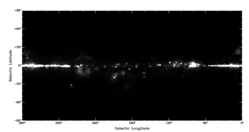
Figure 1: The WMAP free-free map. Note the $\sim 60$ roughly spherical sources, which we associate with massive star clusters.

We present evidence that the bulk of the ELD is associated with photons emitted from massive clusters not previously identified. We are motivated by the distribution of free-free emission in the WMAP free-free map, shown in figure 1, and by comparison of higher resolution radio images, e.g., Whiteoak et al. (1994); Cohen & Green (2001) with GLIMPSE (Benjamin et al., 2003) and MSX (Price et al., 2001) data.

In this paper, we determine the star formation rate in our galaxy using the free-free flux measured by the Wilkinson Microwave Anisotropy Probe (WMAP). We describe our data processing and source identification and extraction methods in §2. By comparing to catalogs of H II regions with known distance, we estimate the distance to the WMAP sources in §3. The H II catalogs are known to be biased against H II regions at large distances; we follow Mezger (1978) and Smith et al. (1978) and crudely account for this by calculating the luminosity of the nearest half of the galaxy, and then doubling the result to find the total $L_{\nu}$. In §4 we examine GLIMPSE images to solidify our identifications; in this process we identify $5-75\,{\rm pc}$ bubbles associated with the bulk ($>75\%$) of the emission. We show that the bubbles and the free-free emission are both powered by massive central star clusters. We derive the ionizing flux $Q$ and the star formation rate of the Galaxy in §5. Half the star formation occurs in the nine most massive clusters and their retinue; the central clusters have $M_{*}=4-10\times 10^{4}M_{\odot}$. We discuss our results in §6. In the appendix we describe the machinery needed to convert from ionizing flux $Q$ to star formation rate $\dot{M}_{*}$.

2 MICROWAVE DATA AND WMAP

The only wavelength range in which free-free dominates the emission from the Galactic plane is in the microwave, between 10 and 100 GHz, placing this in the center of the frequency range of cosmic microwave background (CMB) experiments (Dickinson et al., 2003). Synchrotron radiation and vibrational dust emission are also important contributors in this frequency range. The free-free emission is characterized by a spectral index $\beta$, where the antenna temperature T$\propto\nu^{-\beta}$, and $\beta\approx 2.1$. In contrast, the spectral index for synchrotron radiation is $\beta\approx 2.7-3.2$ and for dust emission $\beta\approx 1.5-2$. In order to isolate the free-free component, some form of multi-wavelength fitting technique must be used.

In order to optimize the WMAP measurements of cosmological parameters, the galactic foreground emission had to be accurately characterized. This was done using a Maximum Entropy Model, resulting in maps of the free-free, synchrotron and dust emission (Bennett et al., 2003a).

These models agree with the observed galactic emission to within $1\%$ overall, with the individual synchrotron and dust emission models matching observations to a few percent. In the case of the free-free map, the correlation to the H$\alpha$ map is found to be within 12 percent. This indicates that the MEM process is consistent with H$\alpha$ where the optical depth is less than 0.5 (Bennett et al., 2003a).

The WMAP free-free model is the only single dish all-sky survey of free-free Galactic emission to date, so it is an attractive data base to use to measure the Galactic ionizing photon luminosity and subsequently the Galactic star formation rate.

2.1 Data Processing

We transformed the WMAP free-free maps from an all-sky HEALPix map to multiple tangential projections centered about the galactic plane. The antenna temperature was converted into flux density using the conversion:

$$F_{\nu}=\frac{2k_{B}\nu^{2}}{c^{2}}\Delta T_{A}$$ (1)

where $\nu$ is the frequency of the WMAP band, $k_{B}$ is Boltzman’s constant, $c$ is the speed of light, and $\Delta T_{A}$ is the antenna temperature (Bennett et al., 2003b). To determine all-sky flux statistics, an all-sky Cartesian projection of the free-free maps was produced.

The WMAP beam diameter varies from 0.82 to 0.21 degrees from the K band to the W band. As part of the map making process, all bands were smoothed to a resolution of 1 degree (Bennett et al., 2003a). The characteristic size of most H II regions is of order the smoothed resolution of the foreground maps. Thus we suffer from source confusion from regions with small angular separations. We discuss our method of separating the confused sources in section 2.2, but argue that in many cases, spatially separate H II regions are physically associated.

2.2 Source Identification & Extraction

Sources within the free-free maps were identified using the Source Extractor package from Bertin & Arnouts (1996). The fluxes were measured in the WMAP W band, at 93.5 GHz. After an automated search over the entire map, a few sources were visually identified and extracted. The measured fluxes are isophotal with an assumed background flux level of zero.

Using this method, the smallest extractable flux is approximately 10 Jy, with a number of higher flux objects being unextractable due to confusion within the Galactic Plane. The smallest H II region extracted had a semi-major axis of 0.4 degrees, half the $\sim 1^{\circ}$ beam diameter of the WMAP free-free map. In total, 88 sources have been identified and extracted.

We have also used the two-dimensional version of the ClumpFind routine by Williams et al. (1994), finding that the sensitivity of the isophote parameter provides unreliably variable sizes and structures for each of the H II regions. Henceforth, we use the sources found by the Source Extractor.

3 DISTANCE DETERMINATION

As a first pass at distance determination, we use the source list of Russeil (2003), who lists both Giant Molecular Clouds and H II regions; only the latter are relevant here. In cases where the sources have both a kinematic distance and photometric distance, we use the photometric distance.

Table 3 in Russeil (2003) lists $481$ H II regions; we find $88$ sources, with a much higher total flux. It follows that we have likely confused individual sources in comparison to the Russeil (2003) list. Thus, we have initially assumed that each of the $88$ sources that we have extracted consists of one or more Russeil sources projected onto the same location in the sky. We use the following procedure to separate these confused sources.

First, in $13$ cases we have a source where Russeil has none. In these cases we inspect either MSX or GLIMPSE images to identify likely sources, and use SIMBAD to find any HII regions at promising locations. For example, we find a source at $l=6.38^{\circ}$, $b=+23^{\circ}$, with a flux $246.5\,{\rm Jy}$, having no counterpart in Russeil (2003). We identify this source with the $\zeta$ Ophiuchi diffuse cloud, at a distance of $140\,{\rm pc}$ (Draine, 1986), and find $Q_{ff}=7.4\times 10^{47}\,{\rm s}^{-1}$ from the free-free emission; we use a subscript to denote the origin of the estimated luminosity (the conversion from $L_{\nu}=4\pi D^{2}f_{\nu}$ to $Q$ is given in equation 7). This ionizing photon luminosity is reasonably consistent with the estimated stellar rate $Q_{*}=1.2\times 10^{48}\,{\rm s}^{-1}$ (Panagia, 1973), and suggests that $\sim 35\%$ of the ionizing photons are absorbed by dust grains.

The most outstanding example of a WMAP source with no associated H II region in Russeil (2003) is that at $81.1^{\circ}$, $b=0.5^{\circ}$. This source was, however, mapped by Westerhout (1958), who identified it as part of the Cygnus X region. Examination of the MSX image shows that there are two large bubbles in the region, one centered roughly on Cygnus OB2, one on Cygnus OB9.

We identify the WMAP source at $l=81^{\circ}$ $b=0.5^{\circ}$ with the northeastern wall of a large bubble in the Cygnus region. The bubble contains Cyg OB2 (see also Schneider et al. (2006)). The second bubble lies to the south, and appears to contain Cyg OB9. The boundary between the two bubbles is a shared wall, which contains Russeil (2003) source 118 at $l=78.5^{\circ}$ $b=0.0^{\circ}$. His sources 120 and 121 are in the interior of the northern bubble, near the center of Cyg OB2. The southeastern rim of the southern bubble contains Russeil’s source 115.

We assign a distance $D=1.7\,{\rm kpc}$ Hanson (2003) to both bubbles (and to the WMAP sources at $l=76.0$, $l=78.6$ and $81.1$). We assign the flux from the WMAP source at $l=76.0^{\circ}$ to the southern bubble, and that of the source at $l=81.1^{\circ}$ to the northern bubble. The flux from the wall separating the two bubbles we rather arbitrarily split evenly between the two. Split this way, $Q_{ff}=1.75\times 10^{51}\,{\rm s}^{-1}$ for the northern bubble, and $Q_{ff}=1.04\times 10^{51}\,{\rm s}^{-1}$ for the southern bubble. We find a total free-free flux in the region of $4033\,{\rm Jy}$; Westerhout (1958) finds a total flux of $2520\,{\rm Jy}$ in “point sources” in the region.

We argue that the free-free flux from the vicinity of the northern bubble can easily be powered by Cyg OB2. Counting only the O stars with spectroscopically determined types listed in table five of Hanson (2003) yields 49 O stars with $Q\approx 5\times 10^{50}\,{\rm s}^{-1}$. More recently, Negueruela et al. (2008) find 50 O stars, and suggest that there may be as many as 60-70 in the cluster, allowing for some incompleteness due to the strong reddening. This is equal to the number of O stars in the Carina region as tabulated by Smith (2006), who also gives $Q_{*}=10^{51}\,{\rm s}^{-1}$, which we also adopt for Cyg OB2; the total ionizing flux for the region will be somewhat larger, as there are a number of O and Wolf-Rayet stars with projected locations inside the bubble but outside Cyg OB2.

We suggest that there must be a similar number of O stars in the interior of the southern bubble as well.

Returning to the distance determinations, if there is a unique Russeil (2003) source at the location of a WMAP source, we use his distance as a first guess; there are $43$ such objects, about half the sample. As in the previous case, we then inspect either MSX or GLIMPSE images at the location of the Russeil source. In some cases we find sources we believe to be better candidates than the source in the Russeil catalog.

Finally, in $30$ cases, we find multiple Russeil (2003) objects in the same direction as our WMAP source. We then assign a portion of our measured flux to each of the Russeil objects. We divide up the WMAP flux using the excitation parameter of each Russeil object. The excitation parameter, $U\propto f_{\nu}D^{2}$, compares the ionizing luminosities of the Russeil objects. Using the distances provided by the catalog, we calculate the free-free luminosity of each Russeil object. The result is a separation of the confused WMAP source into individual H II regions with flux, distance, and luminosity corresponding to the Russeil (2003) objects.

Using this method, we are able to assign distances to all but 2 of the 88 regions. (One of the original 13 missing regions corresponds to the Large Magellanic Cloud; we identified 10 using SIMBAD and their distances are given in table 3). We assigned the average distance of the known sources to the remaining two unidentified sources.

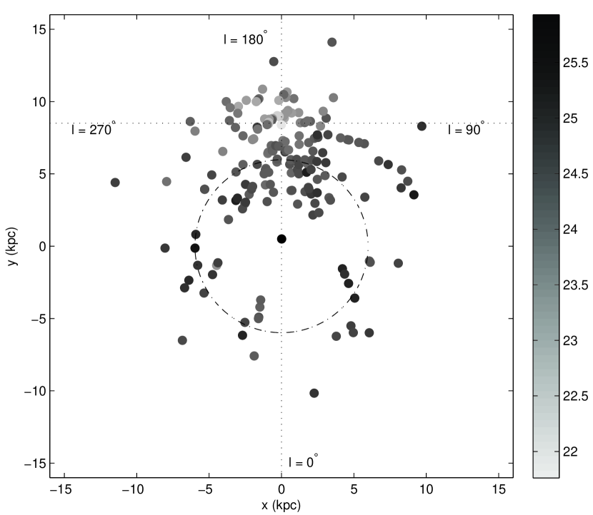
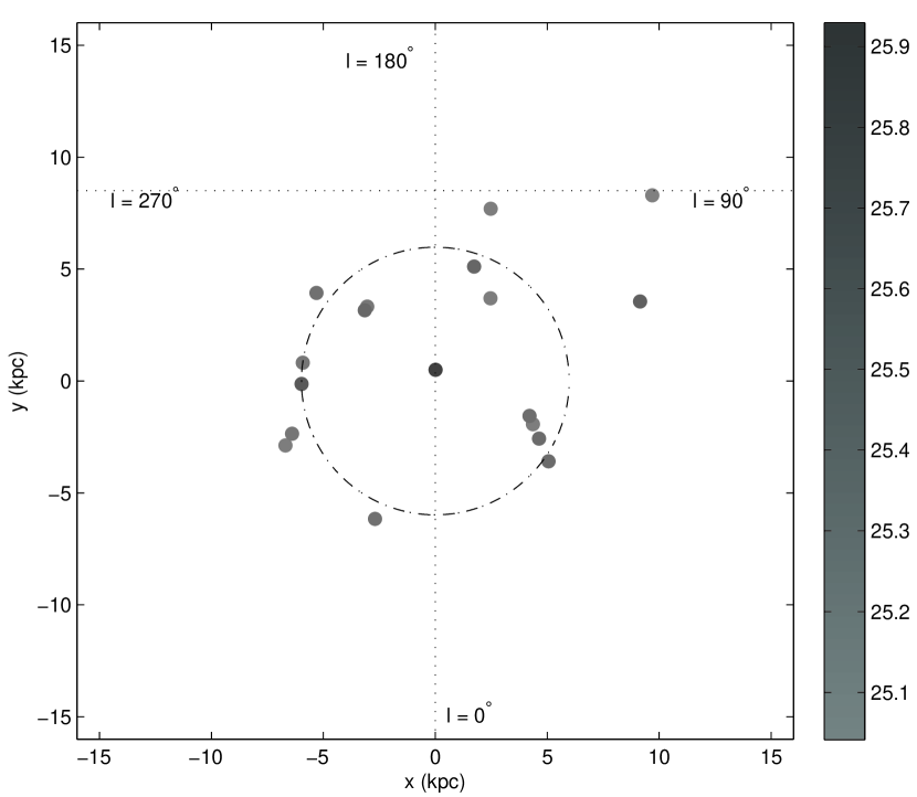
Figure 3: A map of the location of the WMAP H II regions using the distances derived from Russeil (2003) as described in the text. The shade of the points represents the free-free luminosity of the region, log($L_{\nu}$). On the left, we plot all WMAP H II regions, on the right, just the regions with log($L_{\nu}$) $>$ 25 ($Q\gtrsim 10^{51}$). A bias against distant sources is apparent.

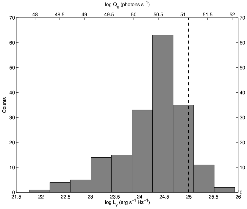
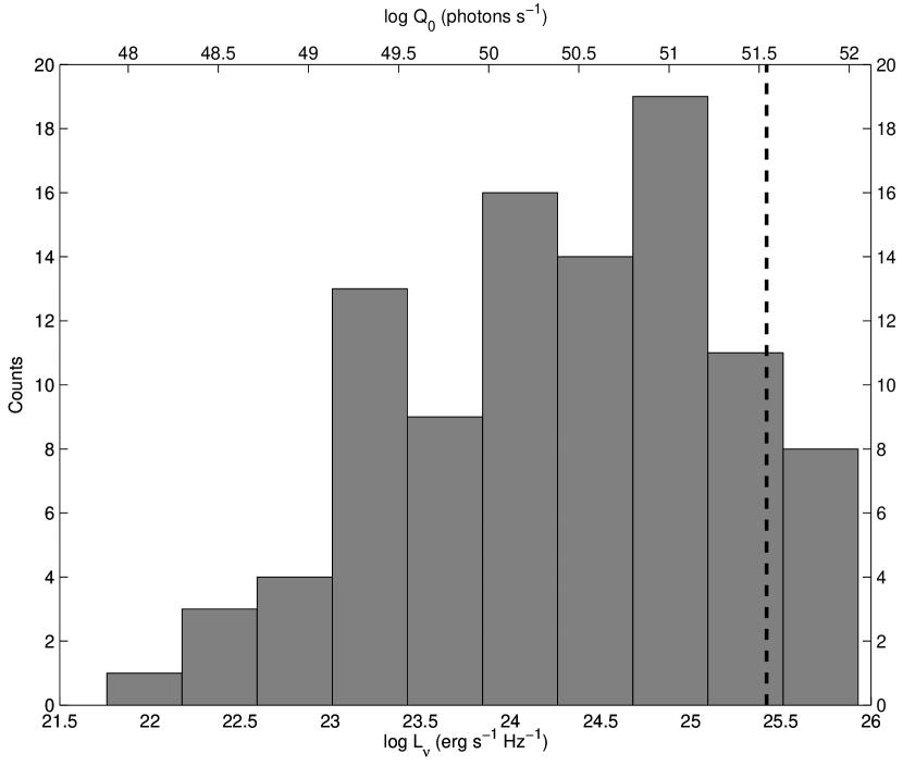
Figure 4: a) The distribution of free-free luminosity of the WMAP H II regions within the galaxy, with the corresponding ionizing luminosity indicated on the top axis. The number of sources at low flux is reduced by confusion. The dashed line indicates the half luminosity line, where the sum of the luminosity of the sources to the right of this line is equal to half the total measured luminosity in the galaxy. The slope on the luminous end is ($dN/dL_{\nu}\sim L_{\nu}^{-\alpha}$) $\alpha=1.9\pm 0.1$. b) The distribution for our clumped sources. The slope on the luminous end is $\alpha=-1.7\pm 0.2$.

We list 183 H II regions in table 3. For all confused sources, the galactic coordinates, semimajor and semiminor axis sizes are for the WMAP source, not the individual H II regions. Maps of these regions are presented in figures 1, 2 and 3. The distribution of free-free luminosities $dN/dL$ of these regions is presented in figure 4.

3.1 WMAP sources, the ELD, and dispersion measures

The WMAP free-free sources range in radius (or semimajor axis) from $0.4^{\circ}$ to $10^{\circ}$. The latter is the fitted radius for the nearby H II region S264 (around $\lambda$ Orionis) at $l=195.05^{\circ}$, $b=-11.995^{\circ}$, $D=400\,{\rm pc}$ (Fich & Blitz, 1984). A visual inspection yields a radius $\sim 5^{\circ}$ or $35\,{\rm pc}$, closer to the radius $r=45.5\,{\rm pc}$ given by Fich & Blitz. As noted above, the effective beam diameter for the free-free map is $\sim 1^{\circ}$. Six sources have mean angular radii (the geometric mean of the semimajor and semiminor axes) smaller than the effective beam radius; these are likely to be unresolved. The physical radii range from $\sim 6\,{\rm pc}$ for $\zeta$ Ophiuchi to $\sim 150\,{\rm pc}$, with a mean radius $\langle r\rangle\sim 55\,{\rm pc}$. We find a filling factor $\phi_{HII}\approx 5\times 10^{-3}$, where $\phi_{HII}$ is the ratio of the (summed) free-free source volume divided by the volume of the galactic disk assuming disk radius $R=8\,{\rm kpc}$ and scale height $H=200\,{\rm pc}$.

The ionizing luminosities fall in the range $10^{48}\,{\rm s}^{-1}<Q<1.8\times 10^{52}\,{\rm s}^{-1}$, with $\langle Q\rangle=2\times 10^{51}$. The median $Q=2.8\times 10^{50}\,{\rm s}^{-1}$ (all these values are uncorrected for dust absorption).

We can determine the mean electron density for each source from the expression

$$n_{e}=\sqrt{3Q\over 4\pi r^{3}\alpha(H^{+})\phi},$$ (2)

where $\alpha(H^{+})=3.57\times 10^{-13}\,{\rm cm}^{3}\,{\rm s}^{-1}$ is the Hydrogen recombination coefficient (Osterbrock, 1989) and $\phi$ is the filling factor of ionized gas in a given WMAP source region. The electron density ranges from $n_{e}\approx 1\phi^{-1/2}\,{\rm cm}^{-3}$ to $n_{e}\approx 35\phi^{-1/2}\,{\rm cm}^{-3}$, with a mean $n_{e}=9\phi^{-1/2}\,{\rm cm}^{-3}$. The density averaged over the disk (i.e., multiplying by the volume filling factor $\phi_{HII}$) is $\langle n_{e}\rangle\approx 0.05\,{\rm cm}^{-3}$. The typical dispersion measure through a WMAP source is $DM\approx 500\,{\rm cm}^{-3}\,{\rm pc}$.

The mean mass of ionized gas in a WMAP source is $3\times 10^{5}\phi^{1/2}M_{\odot}$; the largest sources, with $Q\approx 5\times 10^{51}\,{\rm s}^{-1}$, have an ionized gas mass $\sim 10^{6}\phi^{1/2}M_{\odot}$.

The density-weighted scale height of the sources is $H_{HII}=145\,{\rm pc}$.

Recall that the Taylor & Cordes (1993) model for the inner Galaxy had two components, with scale heights of $150\,{\rm pc}$ and $300\,{\rm pc}$, similar to the scale height we find for WMAP H II sources. The mean density of the WMAP sources, averaged over the inner Galaxy (i.e., multiplied by the filling factor $\phi_{HII}$) is $n_{e}=0.05\,{\rm cm}^{-3}$, compared to the Taylor & Cordes (1993) model values $0.1\,{\rm cm}^{-3}$ and $0.08\,{\rm cm}^{-3}$ for the inner annulus and spiral arms, respectively. Following McKee & Williams (1997), we identify the ELD (the sum of the WMAP sources) with the arm and annulus components for the Taylor & Cordes (1993) model.

3.2 Accounting for the H II region distance bias, and for diffuse emission

We noted above that catalogs of H II regions are known to be biased against distant objects, a result apparent in figure 3. We follow Mezger (1978); Smith et al. (1978); McKee & Williams (1997) and account for this by doubling the luminosity of sources in our half of the Galaxy. This results in

$$L_{\nu,sources}=1.2\times 10^{27}\,{\rm erg\,\,s}^{-1}\,{\rm Hz}^{-1}.$$ (3)

There is a selection effect against low flux sources (less than $\sim 10\,{\rm Jy}$), as mentioned above, due to the source extraction process. The luminosity of a $10\,{\rm Jy}$ source at $15\,{\rm kpc}$ is $2.6\times 10^{24}\,{\rm erg\,\,s}^{-1}\,{\rm Hz}^{-1}$, or $Q=3.5\times 10^{50}\,{\rm s}^{-1}$, about one fifth that of the ionizing flux of Carina. Since the number counts of free-free sources in ground based surveys do not increase much with decreasing flux, such sources do not contribute much to the total free-free luminosity of the galaxy.

On the other hand, there does appear to be a diffuse component to the WMAP free-free sky map (diffuse even compared to the ELD). The total flux over the entire sky is $f_{\nu}=54211.6\,{\rm Jy}$, while that in WMAP sources is $36043.0\,{\rm Jy}$. We give a rough accounting of this emission by assuming that it arises from gas that has the mean distance of the sources, i.e., we multiply the free-free luminosity emitted by the WMAP sources by the ratio $54211.6/36043\approx 1.5$ to find our final estimate for the Galactic free-free luminosity

$$L_{\nu}=1.8\times 10^{27}\,{\rm erg\,\,s}^{-1}\,{\rm Hz}^{-1}.$$ (4)

4 BUBBLES, H II REGIONS, AND MASSIVE STAR CLUSTERS

We show in this section that many of the H II regions listed in Russeil (2003) and earlier compilations are physically connected. In particular, when several sources appear within $\lesssim 1^{\circ}$ on the sky, and have radial velocities within $\Delta v_{r}\approx\pm 10\,{\rm km\,\,s}^{-1}$, examination of Spitzer band 4 GLIMPSE ($8\,\mu{\rm m}$) images reveal large ($10-100\,{\rm pc}$) bubbles, with the H II regions arrayed around the rim of the bubble. We interpret these bubbles as radiation and H II gas pressure driven structures powered by a central massive cluster. Here we give one example; more will be presented in a forthcoming paper.

4.1 WMAP sources are powered by massive star clusters

There are several arguments that the WMAP sources, and their enclosed, apparently empty large bubbles actually contain the largest star clusters in the Milky Way.

The first is the very large ionizing fluxes found using WMAP, $Q\approx 3-10\times 10^{51}\,{\rm s}^{-1}$, for the top 10 or so sources. These sources have WMAP-determined radii of order $100\,{\rm pc}$, so either there are $\sim 3-10$ Carina size clusters all within $100\,{\rm pc}$, and $dN_{cl}/dM$ is very different than we believe, or there is a single dominant cluster.

The second argument is provided by the shape of the GLIMPSE and MSX $8\,\mu{\rm m}$ bubbles inside the WMAP sources. The bubbles are elliptical, with axis ratios one to two or so. This argues for a single massive cluster, which dominates the luminosity of the region.

The third argument is that many of the bubbles show prominent pillars pointing back to a single location in the bubble, again consistent with a single dominant source.

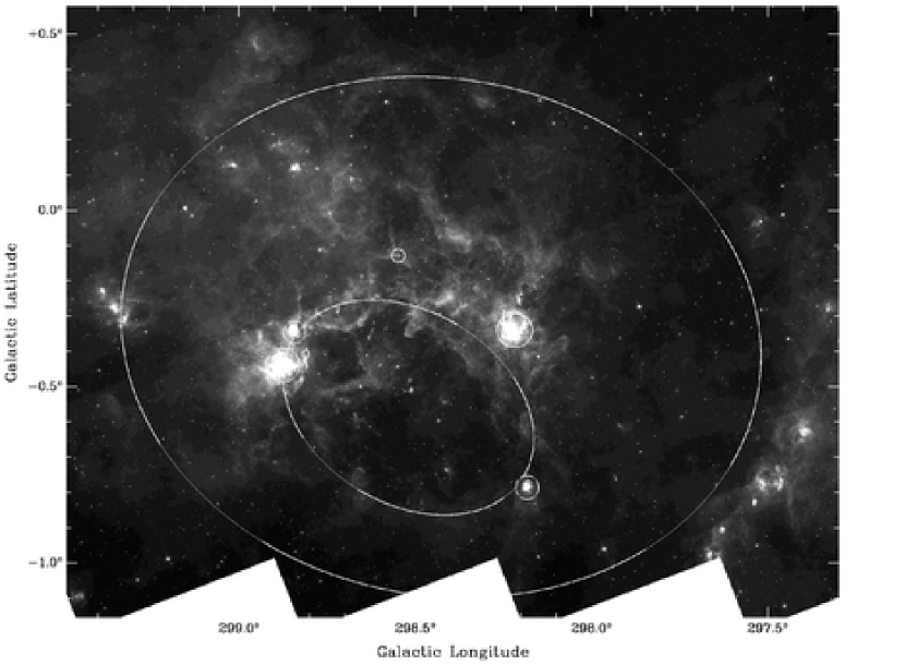
Figure 5: The GLIMPSE $8\,\mu{\rm m}$ image in the direction of WMAP free-free source G298.4-0.4. The large white ellipse shows the WMAP source found by Source Extractor. We find a bubble in the GLIMPSE image, which we approximate with the smaller of the two white ellipses, having semimajor axis $a=1370^{\prime\prime}$ and semiminor axis $b=892^{\prime\prime}$. We have set the intensity and contrast to show the faint bubble outline, resulting in saturated H II regions. Large pillars are evident at $l=298.67^{\circ}$ $b=-0.75^{\circ}$ and $l=298.5^{\circ}$, $b=-0.35^{\circ}$. Also shown (by white circles) are the H II regions listed in table 2; the velocities range from $+16\,{\rm km\,\,s}^{-1}$ to $+30.3$. We interpret this as a bubble expansion velocity of $\sim 7\,{\rm km\,\,s}^{-1}$. The distance to the H II regions is $D\approx 11.7\,{\rm kpc}$.

Finally, we present a quantitative argument for WMAP source G298.3-0.34, showing that there should be a massive cluster $M_{*}\approx 4\times 10^{4}M_{\odot}$ providing the bulk of the ionizing radiation. Along the way we show that the classical giant H II regions associated with this region are powered by compact star clusters with masses $Q\approx 7\times 10^{50}\,{\rm s}^{-1}$, and $M_{cl}\approx 10,000M_{\odot}$. The total $Q\approx 7.7\times 10^{51}\,{\rm s}^{-1}$ for the region; we show that this most likely arises from a cluster at the location pointed to by the giant pillars in figure 5, near $l=298.66^{\circ}$, $b=-0.51^{\circ}$.

Cohen & Green (2001) have shown that the 8 micron emission traces free-free emission well. This allows us to use the $8\,\mu{\rm m}$ images to examine the WMAP sources with much higher resolution.

Figure 5 shows the GLIMPSE image in the direction of the WMAP free-free source G298.4-0.4. SIMBAD lists 7 HII regions within $0.5$ degrees of the center of the bubble (at $l=298.5^{\circ}$, $b=-0.556^{\circ}$); we interpret 2MASX J12100188-62500 to be the same source as [GSL2002] 29, and [WMG70] 298.9-00.4 to be the same source as [CH87] 298.868-0.432. The five unique sources are marked by circles in figure 5 (see table 2). The H recombination line radial velocities range from $+16\,{\rm km\,\,s}^{-1}$ to $+30.3\,{\rm km\,\,s}^{-1}$, with a mean around $+23\,{\rm km\,\,s}^{-1}$. Given the arrangement of sources around the wall, and the range of radial velocities, we interpret the source as an expanding bubble, with mean $r_{bubble}\approx 55(D/10\,{\rm kpc})\,{\rm pc}$ and expansion velocity $\sim 7\,{\rm km\,\,s}^{-1}$. We interpret the H II regions around the rim as triggered star formation. The two largest H II regions on the rim, G298.227-0.340 and G298.862-0.438, have fluxes $f_{\nu}\approx 47\,{\rm Jy}$ and $42\,{\rm Jy}$, corresponding to $Q\approx 7.5\times 10^{50}(D/10\,{\rm kpc})\,{\rm s}^{-1}$ and $6.6\times 10^{50}(D/10\,{\rm kpc})\,{\rm s}^{-1}$. The total flux from the H II regions on the rim is $111\,{\rm Jy}$, compared to the WMAP flux of $313\,{\rm Jy}$. We suggest that there is a massive cluster ($Q\approx 3-5\times 10^{51}\,{\rm erg\,\,s}^{-1}$, or $M_{*}\approx 5\times 10^{4}M_{\odot}$) in the interior of the bubble; the pillars point to the location of the cluster.

We note that even so-called “giant H II regions” are spatially compact, of order a few to ten parsecs in radius (e.g., Conti & Crowther (2004)); the two classical giant H II regions, [CH87] 298.868-0.432 (G298.9-0.4 here) and [GSL2002] 29 (G298.2-0.3) are prominent in the $8\,\mu{\rm m}$ GLIMPSE image, and have radii $3.8$ arcminutes, or $\sim 10(D/10\,{\rm kpc})\,{\rm pc}$ in $6\,{\rm cm}$ radio maps (Conti & Crowther, 2004). Radial profiles from the centers of the $8\,\mu{\rm m}$ sources show the $1/R$ surface brightness profiles expected from point sources; see figure 6. These giant H II regions cannot be responsible for the much more extended $8\,\mu{\rm m}$ emission seen in figure 5 and plotted in figure 6. Nor can the two giant H II regions explain the WMAP free-free emission, which has $r=0.9^{\circ}\approx 160(D/10\,{\rm kpc})\,{\rm pc}$ for G298.

The surface brightness profile around the large bubble also shows a $1/R$ shape at large radii ($r\gtrsim 0.5^{\circ}$). Inside the bubble the surface brightness is generally flat, but with a number of peaks, culminating in the large peak at $r\sim 0.4^{\circ}$, corresponding to the bubble wall. The total $8\,\mu{\rm m}$ luminosity is dominated not by the known H II regions, but by the large scale emission associated with and surrounding the bubble. Figure 6 shows the surface brightness profiles of the two brightest H II regions associated with G298; recall that both lie on the rim of the large bubble. Both profiles merge into the background at $r\sim 0.3^{\circ}\approx 50\,{\rm pc}$. The figure also shows the azimuthally averaged radial surface brightness profile from the putative location of the massive cluster at $l=298.66^{\circ}$, $b=-0.507^{\circ}$. In converting from degrees to parsecs, labeled along the top of the figure, we have assumed a distance $D=10\,{\rm kpc}$ to the object; $D=11.7\,{\rm kpc}$ for $v=+23\,{\rm km\,\,s}^{-1}$ in this direction.

The figure shows that neither of the classical H II regions can be responsible for the large scale ($\sim 200\,{\rm pc}$) diffuse emission. We say this because the $1/R$ scaling for the smaller sources extrapolates to a very low surface brightness at $R\gtrsim 40\,{\rm pc}$. It also suggests that a much more luminous source must be embedded in the bubble interior. The surface brightness of the entire region also falls off as $1/r$ from the point $l=298.66^{\circ}$ $b=-0.507^{\circ}$, as expected if there is a massive cluster near or at this location. It follows that the total $8\,\mu{\rm m}$ luminosity is at least $\sim 3.5$ times that of G298.9-0.4 (the ratio of the surface brightness at large radii in the least squares fits) and $5$ times that of G298.2-0.3; if the emission associated with the H II regions does not extend to the edge of the observed $8\,\mu{\rm m}$ emission, their contribution to the total flux will be smaller.

The azimuthal averaging leads to an artificially thick bubble wall; surface brightness measurement along radial lines show that the radial thickness of the bubble wall is $\Delta r\sim 4(D/10\,{\rm kpc})\,{\rm pc}$, about $20\%$ of the bubble radius.

We noted above that the WMAP free-free source G298 has a radius of $r\approx 160(D/10\,{\rm kpc})\,{\rm pc}$, similar to the radius $200(D/10\,{\rm kpc})\,{\rm pc}$ of the $8\,\mu{\rm m}$ source we find, once again illustrating the correlation between $8\,\mu{\rm m}$ emission and free-free emission.

The total free-free flux in the region is $312\,{\rm Jy}$, compared to $47.4\,{\rm Jy}$ for G298.2-0.3 ($\sim 1/6$ of the total) and $42.4\,{\rm Jy}$ ($1/7$) for G298.9-0.4; note that these ratios are roughly consistent with the $8\,\mu{\rm m}$ flux ratios. We estimate a total flux of $\sim 110\,{\rm Jy}$ for all the classical H II regions in the area, leaving $202\,{\rm Jy}$, which we attribute to the massive central cluster. We inferred above that the cluster has an ionizing luminosity $Q=5\times 10^{51}(D/10\,{\rm kpc})\,{\rm s}^{-1}$, and a stellar mass $M\approx 5\times 10^{4}(D/10\,{\rm kpc})M_{\odot}$, similar to that of Westerlund 1.

Thus we have a slightly different interpretation of the ELD than Lockman (1976) and Anantharamaiah (1985a, b), at least for our most luminous WMAP sources (recall that these dozen or so sources supply the bulk of the ionizing luminosity of the Galaxy). In these sources, the majority of the ionizing flux is produced by a massive star cluster ($M\sim 5\times 10^{4}M_{\odot}$ or larger). These clusters excite free-free and $8\,\mu{\rm m}$ emission out to $50-200\,{\rm pc}$. They have also blown $\sim 10-100\,{\rm pc}$ bubbles in the surrounding ISM, as seen in Spitzer or MSX images. The rims of the bubbles contain triggered star formation regions, which are younger than the central clusters. Because the triggered clusters are younger, and substantially less luminous (typically by a factor of five), they have not blown away their natal gas. As a result, they appear as very high surface brightness free-free sources in classical radio emission catalogs (and as bright $8\,\mu{\rm m}$ sources).

While these young, compact sources are bright and hence easily identified, they are not the source of the ionizing photons in the ELD. Instead, the massive central clusters are the source of the ionizing photons powering the ELD; ionizing photons leak out of the bubbles in all directions, since the bubble walls are far from uniform.

Using this definition of an H II region (treating all the H II regions associated with a GLIMPSE bubble as one region) alters the luminosity function. This new luminosity function is shown in the right panel of figure 4. At the high luminosity end we find $dN/dL\sim N^{-1.7\pm 0.2}$, i.e., most of the luminosity (and stellar mass) is in massive sources ($\alpha=2$ corresponds to equal numbers per logarithmic luminosity bin). Half the luminosity due to sources is in the $9$ most luminous objects, with $Q>3.2\times 10^{50}\,{\rm s}^{-1}$ (not corrected for dust absorption). These sources have luminosities similar to that of the Galactic center, $L_{\nu}>3\times 10^{25}\,{\rm erg}\,{\rm Hz}^{-1}$, or $Q>7\times 10^{51}\,{\rm s}^{-1}$. This corresponds to cluster masses $M_{cl}>10^{5}M_{\odot}$, ranging up to $2.6\times 10^{5}M_{\odot}$.

Kennicutt et al. (1989) survey nearby galaxies and construct H$\alpha$ luminosity functions; they find a range of values for $\alpha$ between $1.5$ and $2.5$, with values below $2$ being slightly more prevalent. McKee & Williams (1997) refit the data presented in Kennicutt et al. (1989) using truncated power law fits, and find a lower range, $1.4<\alpha<2.3$, with a mean $\alpha=1.75\pm 0.23$.

5 IONIZING LUMINOSITIES OF H II REGIONS AND THE GALACTIC STAR FORMATION RATE

The emissivity of the free-free flux from an ionizing region is given by:

$$\epsilon^{ff}_{\nu}=\frac{2^{5}\pi e^{6}}{3m_{e}c^{3}}\left(\frac{2\pi}{3km_{e}}\right)^{1/2}T^{-1/2}Z^{2}n_{e}n_{i}e^{-h\nu/kT}g_{ff}$$ (5)

where $Z$ is the charge per ion, $T$ is the electron temperature, $n_{e}$ and $n_{i}$ are electron and ion density respectively, and $g_{ff}$ is the Gaunt factor. For a fully ionized H II region, we adopt $n_{e}=n_{i}$ and $Z=1$. Further, we adopt an electron temperature, $T_{e}=7000\,{\rm K}$ for H II regions, and a Gaunt factor $g_{ff}=3.3$ (Sutherland, 1998). At radio frequencies we approximate this as $\epsilon^{ff}_{\nu}=\epsilon_{0}n_{e}^{2}$, where $\epsilon_{0}=2.7\times 10^{-39}\,{\rm g}\,{\rm cm}^{5}\,{\rm s}^{-3}\,{\rm Hz}^{-1}$.

To keep an isotropic H II region ionized, the total number of ionizing photons required is:

$$Q_{tot}=\int n_{e}^{2}\alpha(H^{+})dV,$$ (6)

where $V$ is the volume of the ionized region.

The total ionizing luminosity (in photons/s) of a given H II region is then

$$Q_{tot}={\alpha(H^{+})\over\epsilon_{o}}L_{\nu}\approx 1.33\times 10^{26}L_{\nu}\,{\rm s}^{-1}.$$ (7)

Using this expression we find the ionizing luminosity of the galaxy, before correction for absorption by dust, is $Q_{tot}=2.34\times 10^{53}\textrm{ photons}\,{\rm s}^{-1}$.

The final step is to correct for the effect of absorption by ionizing photons by dust grains. Following McKee & Williams (1997), we multiply by $1.37$, and find

$$Q_{tot}=3.2\times 10^{53}\textrm{ photons}\,{\rm s}^{-1}.$$ (8)

5.1 Star Formation Rate

To estimate the star formation rate from $Q$, we follow Mezger (1978) and McKee & Williams (1997), and use the expression

$$\dot{M}_{*}=Q{\langle m_{*}\rangle\over\langle q\rangle}{1\over\langle t_{Q}\rangle},$$ (9)

where $\langle q\rangle$ is the ionizing flux per star averaged over the initial mass function, and $\langle m_{*}\rangle$ is the mean mass per star, in solar units. The quantity $\langle t_{Q}\rangle$ is the ionization-weighted stellar lifetime, i.e., the time at which the ionizing flux of a star falls to half its maximum value, averaged over the IMF; all the averaged terms are discussed in the appendix.

All of these averaged quantities depend on the initial mass function (IMF) of the stars, in particular on the high mass slope $\Gamma$ of the IMF, as discussed in the appendix; as an example, and to fix notation, the Salpeter (1955) IMF is given by $\xi(m)\equiv mdN/dm={\cal N}m^{-\Gamma}$, with $\Gamma=1.35$.

Using the stellar evolution models of Bressan et al. (1993) we find $\langle t_{Q}\rangle=3.9\times 10^{6}\,{\rm yr}$ (for $\Gamma=1.35$). This is slightly longer than the ionizing flux-weighted main sequence lifetime $\langle t_{ms}\rangle=3.7$ Myrs used by McKee & Williams (1997), which is in turn somewhat larger than the $3$ Myrs used by Mezger (1978). This value is only weakly dependent on $\Gamma$.

The mean ionizing flux per solar mass, $\langle q\rangle/\langle m_{*}\rangle$, is much more problematic; it depends sensitively on $\Gamma$. Figure 7a shows $\langle q\rangle/\langle m\rangle$ using $Q(m)$ as determined by Martins et al. (2005) (the solid line) and as given by Vacca et al. (1996) (their evolutionary masses); in making this figure we used the Muench et al. (2002) IMF. The difference between the two estimates for $Q(m)$ results in a difference in $\langle q\rangle/\langle m\rangle$ of $\sim 10\%$. The filled square represents our favored value

$${\langle q\rangle\over\langle m_{*}\rangle}=6.3\times 10^{46}\,{\rm s}^{-1}\,M_{\odot}^{-1},$$ (10)

at $\Gamma=1.35$.

For the Muench et al. (2002) IMF $\langle m_{*}\rangle=0.71$ when $\Gamma=1.35$; $\langle q\rangle=4.5\times 10^{46}\,{\rm s}^{-1}$. This is a factor $5$ larger than the value quoted by McKee & Williams (1997), $\langle q\rangle=8.9\times 10^{45}\,{\rm s}^{-1}$; this difference is not primarily a result of our using different expressions for $Q(m)$, since the dashed line uses Vacca et al. (1996), as did McKee & Williams (1997) used.

We show that this factor of $5$ arises mostly from the use of a different IMF, with two contributing factors, the use of a different value of $\Gamma$, and a different IMF shape, so that McKee & Williams (1997) finds fewer massive stars at a fixed value of $m$, even when $\Gamma$ is chosen to be the same for the two IMFs; in this comparison, we choose $\Gamma=1.5$ to match their work.

Figure 7b shows the mean ionizing flux per solar mass for the Scalo-type IMF used by McKee & Williams (1997) (dot-dashed line), the Muench et al. (2002) IMF (solid line) , and the Chabrier (2005) IMF (long-dash line), all as a function of $\Gamma$. In making this plot we have used the relation between $Q$ and evolutionary mass given by Vacca et al. (1996), so that the dot-dashed curve goes through the McKee & Williams (1997) result.

From this plot we can see that the variation in $\Gamma$ is responsible for about a factor of $2$ out of the total factor $5$ difference; the rest comes from the different shape of the IMF, with the more recent IMFs (Muench et al. (2002) or Chabrier (2005)) having many fewer low mass stars, or alternately, more high mass stars, even for fixed $\Gamma$.

The figure shows that small changes in $\Gamma$ lead to large changes in the inferred star formation rate. Recent observations of young massive clusters have suggested that $\Gamma$ varies from the Salpeter value (Stolte et al., 2002; Harayama et al., 2008); if confirmed, these variations, combined with the results presented here, would lead to large variations in the estimated star formation rate of the Galaxy.

Using the ionizing flux given by Martins et al. (2005), we can integrate over a Muench et al. (2002)-like IMF (eqn. A3), with $\Gamma$ as a free parameter. In the appendix we find

$${\langle q\rangle\over\langle m_{*}\rangle}\approx 6.3\times 10^{46}\left(m_{Q}^{1.35-\Gamma}\right)\,{\rm s}^{-1}M_{\odot}^{-1},$$ (11)

where $m_{Q}\approx 35M_{\odot}$ is the location of the break in a powerlaw fit to $Q(m)$ (figure 8).

Finally, we find a star formation rate for the Milky Way of

$$\dot{M}_{*}=4.1\times 10^{-54}Q=1.3M_{\odot}\,{\rm yr}^{-1}.$$ (12)

Using the McKee & Williams (1997) value of $\Gamma=1.5$ results in $\dot{M}_{*}=2.2M_{\odot}\,{\rm yr}^{-1}$, lower than their $4.0M_{\odot}\,{\rm yr}^{-1}$ due to the different form of the IMF (aside from the high mass slope $\Gamma$) and our use of the Martins et al. (2005) temperature scale; as seen in figure 7, using their IMF and Vacca et al. (1996), we recover $\dot{M}_{*}\approx 4M_{\odot}\,{\rm yr}^{-1}$. Using the Muench et al. (2002) slope, the result is $0.9M_{\odot}\,{\rm yr}^{-1}$.

5.2 The Magellanic Clouds

We were able to measure the free-free flux of the Large Magellanic Cloud (LMC) and Small Magellanic Cloud (SMC), and thus can provide a star formation rate for each of these galaxies. We find $f_{\nu}=92.2\,{\rm Jy}$ for the LMC and $f_{\nu}=6.4\,{\rm Jy}$ for the SMC. We adopt a distance to the LMC of $D=48.1\,{\rm kpc}$ (Macri et al., 2006), and $D=60.6\,{\rm kpc}$ for the SMC (Hilditch et al., 2005). This leads to free-free luminosities of $L_{\nu}=2.54\times 10^{26}\,{\rm erg}\,{\rm s}^{-1}\,{\rm Hz}^{-1}$ and $L_{\nu}=2.81\times 10^{25}\,{\rm erg}\,{\rm s}^{-1}\,{\rm Hz}^{-1}$ respectively. Using eqns. 7 and 12 we determine a SFR of $0.14M_{\sun}\,{\rm yr}^{-1}$ for the LMC and $0.015M_{\odot}\,{\rm yr}^{-1}$ for the SMC. Our estimate for the LMC is slightly lower than but consistent with the estimate of $0.25M_{\odot}\,{\rm yr}^{-1}$ found using H$\alpha$ and MIPS data by Whitney et al. (2008). Our estimate for the LMC is significantly lower than the H$\alpha$ estimate of 0.08 M_☉ yr^-1 determined by Kennicutt & Hodge (1986) and the IR estimate of 0.05 M_☉ yr^-1 determined by Wilke et al. (2004).

6 SUMMARY & DISCUSSION

We have combined the WMAP free-free map with previous determinations of distances to H II regions to measure the ionizing flux of the Galaxy. We find $Q=3.2\times 10^{53}\,{\rm s}^{-1}$, in agreement with previous determinations. We found $88$ sources responsible for a flux of $36043\,{\rm Jy}$, out of a total flux of $54211.6\,{\rm Jy}$.

The mean WMAP source radius is $\sim 60\,{\rm pc}$. Inspection of Spitzer GLIMPSE images and MSX images shows that diffuse $8\,\mu{\rm m}$ emission, which closely tracks the free-free emission, gives sizes consistent with the WMAP sizes, e.g., figure 6, suggesting that many of the WMAP sources are in fact resolved.

The mean source electron density is $9.3\,{\rm cm}^{-3}$; hence the mean dispersion measure across a source is $DM\approx 540\,{\rm cm}^{-3}\,{\rm pc}$; from figure 1 most of the sources are within $\sim 60^{\circ}$ of the galactic center. Thus we identify these sources with the inner galaxy and spiral arm components of the free electron model of Taylor & Cordes (1993). The density weighted scale height of the sources is $114\,{\rm pc}$. The total volume filling factor of of the sources is $\sim 0.005$. Thus the Galactic mean electron density is $\langle n_{e}\rangle\approx 0.045\,{\rm cm}^{-3}$.

We used GLIMPSE and MSX images to study the WMAP sources with higher resolution. We found that the bulk of the Galactic star formation (of order half) occurs in $\sim 10$ sources, with $Q\approx 5\times 10^{51}\,{\rm s}^{-1}$. The $8\,\mu{\rm m}$ images revealed large bubbles, with $r\sim 20\,{\rm pc}$, ranging up to $100\,{\rm pc}$, in most of these sources. We showed that classical giant H II regions associated with the WMAP sources were located in the bubble walls, and interpreted them as triggered star formation. We argued that the bubbles are powered by massive star clusters responsible for the bulk of the ionizing flux in each WMAP source. We estimate that these clusters have masses $M_{*}\approx 4\times 10^{4}M_{\odot}$ or larger.

We note that there are now a number of slightly older (but still young, $10-20$ Myr old) Milky Way clusters known to have masses in this range; examples include Westerlund 1 with $M\sim 5\times 10^{4}M_{\odot}$ (Brandner et al., 2008), the Arches cluster $M\sim 4\times 10^{4}M_{\odot}$ (Figer et al., 1999), and the red supergiant clusters RSGC1 near G25.25-0.15 $M\sim 3\times 10^{4}M_{\odot}$ (Figer et al., 2006), RSGC2 ($l=26.2^{\circ}$ $b=-0.06^{\circ}$) with $M\sim 4\times 10^{4}M_{\odot}$ (Davies et al., 2007), and RSCG3 ($l=29.2^{\circ}$ $b=-0.2^{\circ}$) with $M\approx 3\times 10^{4}M_{\odot}$ (Clark et al., 2009). In a forthcoming paper we show that almost all of our high luminosity WMAP sources, as well as the less luminous sources, are associated with large bubbles seen in GLIMPSE images, and most have fairly compact clusters in the bubble interior.

Lockman (1976) and Anantharamaiah (1985a, b) suggested that the ELD, which we identify with the WMAP sources, and which accounts for the bulk of the free-free emission in the Galaxy, arises from ionizing photons that leak out of H II regions. We agree that the ELD is closely associated with giant H II regions. However, as figure 6 shows, the bulk of the ionizing flux powering the ELD arises from massive clusters in the centers of large bubbles; the giant H II regions are due to smaller (but still large) clusters located in the bubble walls. The massive clusters are not readily identified in free-free maps because they have blown away their natal gas, and so do not produce any high surface brightness emission (either free-free, $8\,\mu{\rm m}$, or even far infrared).

Using recent estimates of $Q(m)$ and the initial mass function $\xi(m)$ of stars, we found a Galactic star formation rate of $\dot{M}_{*}=1.8M_{\odot}\,{\rm yr}^{-1}$. This is somewhat smaller than past determination of the Galactic star formation rate. We showed that all estimates based on measurements of ionizing radiation are highly sensitive to the slope $\Gamma$, where $\xi(m)\sim m^{-\Gamma}$ at high mass. In this case, “high mass” is the critical mass $m_{Q}\approx 40M_{\odot}$ where stellar luminosities approach the Eddington luminosity. Our quoted value of $\dot{M}_{*}$ assumes that $\Gamma=1.35$, the Salpeter value.

Appendix A INITIAL MASS FUNCTIONS, IONIZING FLUXES AND IONIZING LIFETIMES

We collect here the machinery needed to calculate the star formation rate from observations of free-free radio emission, following Smith et al. (1978) and McKee & Williams (1997).

We use four initial mass functions, all written in terms of stellar mass in units of the Solar mass, $m=M/M_{\odot}$, with $0.1\leq m\leq 120$. The first is the Salpeter (1955) IMF,

$$\xi(m)\equiv mdN/dm={\cal N}(\Gamma)m^{-\Gamma}.$$ (A1)

Salpeter found $\Gamma=1.35$.

The second IMF is the McKee & Williams (1997) version of Scalo (1986), which at the high mass end looks like the Salpeter IMF,

$$mdN/dm={\cal N}m^{-\Gamma},$$ (A2)

with ${\cal N}=0.063C_{F}$; they take $C_{F}=1.4$. McKee & Williams (1997) use $\Gamma=1.5$.

Third, we use a modified Muench et al. (2002) IMF:

$$\xi_{M,m_{1}}(m)\equiv m{dN\over dm}=N_{0}\left\{\begin{array}[]{ll}m^{-\Gamma}&m_{U}>m>m_{1}\\ m_{1}^{(0.15-\Gamma)}m^{-0.15}&m_{1}>m>m_{2}\\ m_{1}^{(0.15-\Gamma)}m_{2}^{(-0.73-0.15)}m^{0.73}&m_{2}>m>m_{L}\end{array}\right.$$ (A3)

Muench et al. (2002) found $\Gamma=1.21$ for the Orion region. As indicated above, $m_{U}=120$ and $m_{L}=0.1$. We use $m_{1}=0.6$ as the characteristic break mass.

Finally, we use the Chabrier (2005) IMF

$$\xi(m)=N_{0}\left\{\begin{array}[]{ll}\exp\left\{-{(\log m-\log 0.2)^{2}\over 2\times(0.55)^{2}}\right\}&m_{L}\leq m\leq 1\\ 0.446m^{-\Gamma}&1<m\leq M_{U}\end{array}\right.$$ (A4)

We use the normalization

$$\int_{m_{L}}^{m_{U}}\xi(m){dm\over m}=1.$$ (A5)

In that case the ionizing flux per Solar mass is

$${\langle q_{*}\rangle\over\langle m_{*}\rangle}\equiv\int_{m_{L}}^{m_{U}}Q(m)\xi(m){dm\over m}\Bigg{/}\int_{m_{L}}^{m_{U}}\xi(m)dm,$$ (A6)

where

$$\langle m_{*}\rangle\equiv\int_{m_{L}}^{m_{U}}\xi(m)dm$$ (A7)

is the mean mass per star.

We use both the Vacca et al. (1996) and Martins et al. (2005) compilations of ionizing fluxes as a function of stellar mass; the ionizing flux $Q(m)$ is given per star by both. Since many clusters harbor stars with mass in excess of $100M_{\odot}$, but neither paper models stars with $M>88M_{\odot}$, we have added the result of Martins et al. (2008), who find $Q\approx 10^{50}$ for each of four WN7-8h stars with $\log L/L_{\odot}>6.3$ (all of which they model by stars with $M\gtrsim 120M_{\odot}$; see their table 2 and figure 2). These stars are slightly evolved, but still very young. Figure 8 shows $Q(M_{*})$ for both Vacca et al. (1996) and Martins et al. (2005).

The function $Q(m)\sim m^{4}$ for $15<m\lesssim m_{Q}$ (where $m_{Q}\approx 40$), but $Q(m)\sim m^{1.5}$ for $m>m_{Q}$. The integral $<Q_{*}>(m)\sim mQ(m)\phi(m)\sim m^{1.65}$ for $m<m_{Q}$, and $\sim m^{0.15}$ for larger $m$, indicating that the bulk of the ionizing flux occurs for stars with mass around $m_{Q}$, for all of our IMFs. Doing the integrals on the right hand side of eqn. (A6) from $m_{L}$ to $m_{Q}$ gives

$${\langle q_{*}\rangle\over\langle m_{*}\rangle}\sim m_{Q}^{-(\Gamma+1)},$$ (A8)

which fits the numerical result rather well; it is shown as the dotted line in figure 7.

The ionizing flux-weighted lifetime of a cluster is given by

$$\langle t_{Q}\rangle\equiv\int_{m_{L}}^{m_{U}}Q(m)t(m)\xi(m){dm\over m}\Bigg{/}\int_{m_{L}}^{m_{U}}Q(m)\xi(m){dm\over m},$$ (A9)

where $t(m)$ is the main sequence lifetime of a star of mass $m$.

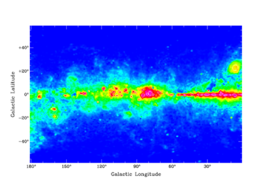
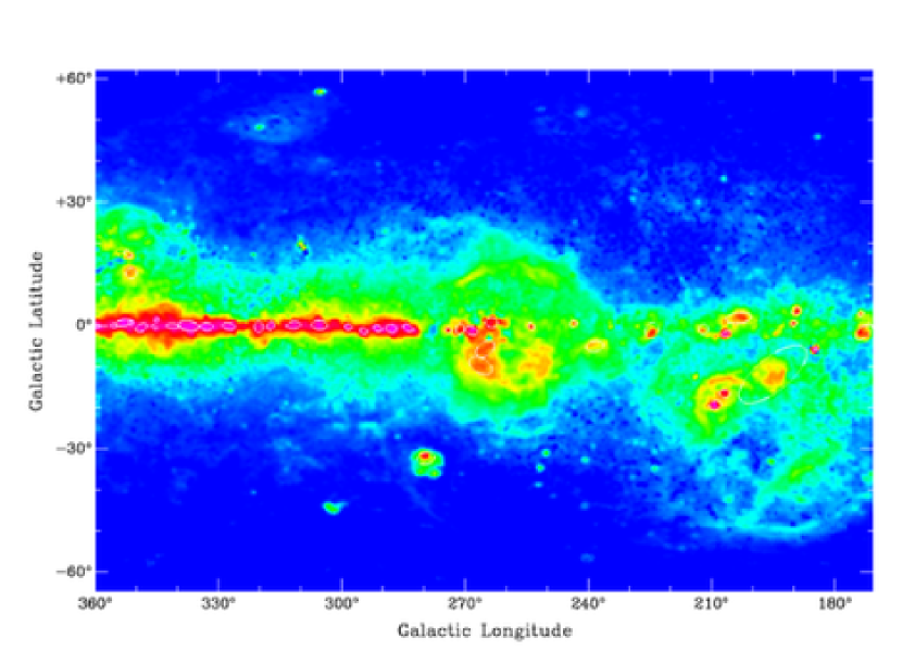
Figure 2: The WMAP free-free map showing the sources found by Sextractor.

Figure 6: The surface brightness (${\rm MJy}{\rm\,sr}^{-1}$) as a function of radius, starting from the apparent location of the cluster ($l=298.66^{\circ}$, $b=-0.507^{\circ}$, thick solid line) and from the two giant H II regions G298.9-0.4 and G298.2-0.3 (thin solid lines; the upper curve near $r=0.1^{\circ}$ is G298.2-0.3). The straight dotted and dashed lines are least squares fits for $0.01^{\circ}<r<0.2^{\circ}$ for G298.9-0.4 and G298.2-0.3; the slopes are $-0.9$ and $-0.98$ i.e., $I(r)\sim 1/r$. Extrapolating to $r=2^{\circ}$, the upper limit for the luminosity of G298.2-0.3 is $\sim 1/4$ that of the region as a whole, while that of G298.9-0.4 is $1/5$ of the total; the ratios found from the free-free emission are somewhat smaller. The fact that the entire region has a luminosity larger than that of the brightest classical H II regions, combined with the presence of a diffuse eight micron emission region much larger than either H II region could illuminate, strongly suggests the presence of a much more luminous star cluster in the interior of the bubble. The interior of the bubble shows little emission, as the gas and dust have been pushed to the bubble wall.

Figure 7: The ionizing flux per solar mass for a massive cluster, plotted as a function of the slope $\Gamma$ of the IMF for large stellar masses; $m_{*}dN/dm_{*}\sim m_{*}^{-\Gamma}$. a) The solid line is the result of using the Martins et al. (2005) expression for $Q(m)$, while the dashed line is the result of using the Vacca et al. (1996) $Q(m)$. The dotted line is the approximation given by eqn. A8. The two open triangles are the results of Smith et al. (1978) ($\Gamma=1.35$) and McKee & Williams (1997) ($\Gamma=1.5$); recall that the latter used the Vacca et al. $Q(m)$. The difference between the solid and dashed lines is about a factor of $1.13$ at $\Gamma=1.35$, so the mismatch between either curve and the triangles is not due to the use of different $Q(m)$. b) Here we plot $\langle q\rangle/\langle m\rangle$ for different IMFs, using the Vacca et al. (1996) $Q(m)$. The dot-dash line uses the McKee & Williams (1997) IMF, so it goes through the open triangle. The solid line represents the Muench et al. (2002) IMF, while the long-dash line is for the Chabrier (2005) IMF—it is almost indistinguishable from the Muench IMF. We note that the ratio between the flux per solar mass for $\Gamma=1.5$ and $1.21$ is $8.37/2.31\sim 3.5$, for all three IMFs. By itself, this dependence on the high-mass slope $\Gamma$ leads to a large uncertainty in the star formation rate as measured by any method that counts ionizing photons, e.g., free-free, H$\alpha$, or [NII] recombination. Variations in the low-mass end of the IMF will only add to this uncertainty.

Figure 8: The ionizing flux $Q$ as a function of stellar mass $M$. The open squares (joined by a dashed line) show the results using the evolutionary masses of Vacca et al. (1996), while the solid squares (joined by a solid line) show the results using those of Martins et al. (2005); both have been supplemented by the addition of a slightly evolved model for a $120M_{\odot}$ star taken from Martins et al. (2008). The slope below $M_{Q}\approx 40M_{\odot}$ for both models is $d\ln Q/d\ln M\approx 4$, while that for $M_{Q}$ is $\approx 1.7$, indicating that the bulk of the ionizing emission for any of our standard IMFs comes from stars with $M\sim M_{Q}$.

Table 1: Galactic Ionizing Flux Measurements

Galactic Ionizing Luminosity $Q$	Reference
${\rm photons}\,{\rm s}^{-1}$
$3.0\times 10^{53}$	1
$2.7\times 10^{53}$	2
$4.7\times 10^{53}$	3
$2.6\times 10^{53}$	4
$3.5\times 10^{53}$	5
$2.6\times 10^{53}$	4
$3.2\times 10^{53}$	6

Note. — (1) Mezger (1978) (2) Gusten & Mezger (1982) (3) Smith et al. (1978) (4) McKee & Williams (1997) (5) Bennett et al. (1994) (6) This work.

Table 2: H II Regions Within $0.5^{\circ}$ of $l=298.5^{\circ}$, $b=-0.556^{\circ}$.

Name	Galactic $l$	Galactic $b$	RA(J2000)	DEC(J2000)	Flux	$v_{r}$	Distance	Ref
	degrees	degrees	hh:mm:ss	deg:mm:ss	Jy	$\,{\rm km\,\,s}^{-1}$	kpc
[KC97c] G298.2-00.8	$298.1869$	$-0.7821$	12:09:03.7	-63:15:46	$2.4$	$+16$	$10.9$	1
[GSL2002] 29	$298.228$	$-0.3308$	12:10:04.0	-62:49:27	$47.4$	$+30.3$	$12.3$	1
[KC97c] G298.6-00.1	$298.5589$	$-0.1141$	12:13:12.6	-62:39:39	$2.8$	$+23$	$11.7$	1
[WMG70] 298.8-00.3	$298.8377$	$-0.3467$	12:15:19.9	-62:55:52	$16.0$	$+25$	$12.0$	2
[CH87] 298.868-0.432	$298.8683$	$-0.4325$	12:15:29.6	-63:01:13	$42.4$	$+25$	$12.0$	1

Note. — (1) Caswell & Haynes (1987) (2) Wilson et al. (1970). Fluxes for [GSL2002] 29 and [CH87] 298.868-0.432 are taken from Conti & Crowther (2004); all others are from Caswell & Haynes (1987)

Table 3: Identified H II Regions

l	b	Semi-Major Axis	Semi-Minor Axis	Free-Free Flux	Distance	Distance Reference	Free-Free Luminosity	Associated Region
		(Degrees)	(Degrees)	(Jy)	(kpc)		(erg s-1 Hz-1)
6.4	23.1	2.5	2.1	247	0.1	-1	1.90E+25	$\zeta$ Oph
6.7	-0.5	1.8	1.2	11	12.3	6	2.00E+24
6.7	-0.5	1.8	1.2	9	13.6	7	2.10E+24
6.7	-0.5	1.8	1.2	6	16.2	8	2.00E+24
6.7	-0.5	1.8	1.2	618	1.6	9	1.90E+24	M8
6.7	-0.5	1.8	1.2	8	12.8	10	1.50E+24
6.7	-0.5	1.8	1.2	281	2.5	11	2.10E+24	W28
6.7	-0.5	1.8	1.2	165	2.7	12	1.40E+24	M20
6.7	-0.5	1.8	1.2	16	13.5	14	3.60E+24
6.7	-0.5	1.8	1.2	76	4.8	15	2.10E+24	W30
10.4	-0.3	0.6	0.4	104	4.3	17	2.30E+24
10.4	-0.3	0.6	0.4	66	14.9	18	1.80E+25	W31
10.4	-0.3	0.6	0.4	85	5.5	19	3.10E+24
10.4	-0.3	0.6	0.4	20	14.0	20	4.80E+24
14.7	-0.5	1.4	0.5	43	4.4	30	1.00E+24

Note. — Table 3 is published in its entirety in the electronic edition of the Astrophysical Journal. A portion is shown here for guidance regarding its form and content.

References

- Anantharamaiah (1985a) Anantharamaiah, K. R. 1985, Journal of Astrophysics and Astronomy, 6, 177
- Anantharamaiah (1985b) Anantharamaiah, K. R. 1985b, Journal of Astrophysics and Astronomy, 6, 203
- Benjamin et al. (2003) Benjamin, R. A., et al. 2003, PASP, 115, 953
- Bennett et al. (1994) Bennett, C. L., et al. 1994, ApJ, 434, 587
- Bennett et al. (2003a) Bennett, C. L., et al. 2003a, ApJS, 148, 97
- Bennett et al. (2003b) Bennett, C. L., et al. 2003b, ApJ, 583, 1
- Bertin & Arnouts (1996) Bertin, E., & Arnouts, S. 1996, A&AS, 117, 393
- Brandner et al. (2008) Brandner, W., Clark, J. S., Stolte, A., Waters, R., Negueruela, I., & Goodwin, S. P. 2008, A&A, 478, 137
- Bressan et al. (1993) Bressan, A., Fagotto, F., Bertelli, G., & Chiosi, C. 1993, A&AS, 100, 647
- Caswell & Haynes (1987) Caswell, J. L., & Haynes, R. F. 1987, A&A, 171, 261
- Chabrier (2005) Chabrier, G. 2005, in The Initial Mass Function 50 Years Later, ed. E. Corbelli & F. Palla (Berlin: Springer), 41
- Clark et al. (2009) Clark, J. S., et al. 2009, arXiv:0903.1754
- Cohen & Green (2001) Cohen, M., & Green, A. J. 2001, MNRAS, 325, 531
- Conti & Crowther (2004) Conti, P. S., & Crowther, P. A. 2004, MNRAS, 355, 899
- Davies et al. (2007) Davies, B. et al. 2007, ApJ, 671, 781
- Draine (1986) Draine, B. T. 1986, ApJ, 310, 408
- Dickinson et al. (2003) Dickinson, C., Davies, R. D., & Davis, R. J. 2003, MNRAS, 341, 369
- Fich & Blitz (1984) Fich, M., & Blitz, L. 1984, ApJ, 279, 125
- Figer et al. (1999) Figer, D. F., Kim, S. S., Morris, M., Serabyn, E., Rich, R. M., & McLean, I. S. 1999, ApJ, 525, 750
- Figer et al. (2006) Figer, D. F. et al. 2006, ApJ, 643, 1166
- Gusten & Mezger (1982) Gusten, R., & Mezger, P. G. 1982, Vistas in Astronomy, 26, 159
- Hanson (2003) Hanson, M. M. 2003, ApJ, 597, 957
- Harayama et al. (2008) Harayama, Y., Eisenhauer, F., & Martins, F. 2008, ApJ, 675, 1319
- Hilditch et al. (2005) Hilditch, R. W., Howarth, I. D., & Harries, T. J. 2005, MNRAS, 357, 304
- Kennicutt et al. (1989) Kennicutt, R. C., Jr., Edgar, B. K., & Hodge, P. W. 1989, ApJ, 337, 761
- Kennicutt & Hodge (1986) Kennicutt, R. C., Jr., & Hodge, P. W. 1986, ApJ, 306, 130
- Lockman (1976) Lockman, F. J. 1976, ApJ, 209, 429
- Macri et al. (2006) Macri, L. M., Stanek, K. Z., Bersier, D., Greenhill, L. J., & Reid, M. J. 2006, ApJ, 652, 1133
- Martins et al. (2008) Martins, F., Hillier, D. J., Paumard, T., Eisenhauer, F., Ott, T., & Genzel, R. 2008, A&A, 478, 219
- Martins et al. (2005) Martins, F., Schaerer, D., & Hillier, D. J. 2005, A&A, 436, 1049
- McKee & Williams (1997) McKee, C. F., & Williams, J. P. 1997, ApJ, 476, 144
- Mezger (1978) Mezger, P. G. 1978, A&A, 70, 565
- Muench et al. (2002) Muench, A. A., Lada, E. A., Lada, C. J., & Alves, J. 2002, ApJ, 573, 366
- Negueruela et al. (2008) Negueruela, I., Marco, A., Herrero, A., & Clark, J. S. 2008, A&A, 487, 575
- Osterbrock (1989) Osterbrock, D. E. 1989, Astrophysics of Gaseous Nebulae and Active Galactic Nuclei (Mill Valley, CA: University Science Books)
- Panagia (1973) Panagia, N. 1973, AJ, 78, 929
- Price et al. (2001) Price, S. D., Egan, M. P., Carey, S. J., Mizuno, D. R., & Kuchar, T. A. 2001, AJ, 121, 2819
- Russeil (2003) Russeil, D. 2003, A&A, 397, 133
- Salpeter (1955) Salpeter, E. E. 1955, ApJ, 121, 161
- Scalo (1986) Scalo, J. 1986, Fund. Cosmic Phys., 11, 1
- Schneider et al. (2006) Schneider, N., Bontemps, S., Simon, R., Jakob, H., Motte, F., Miller, M., Kramer, C., & Stutzki, J. 2006, A&A, 458, 855
- Smith (2006) Smith, N. 2006, MNRAS, 367, 763
- Smith et al. (1978) Smith, L. F., Biermann, P., & Mezger, P. G. 1978, A&A, 66, 65
- Stolte et al. (2002) Stolte, A., Grebel, E. K., Brandner, W., & Figer, D. F. 2002, A&A, 394, 459
- Sutherland (1998) Sutherland, R. S. 1998, MNRAS, 300, 321
- Taylor & Cordes (1993) Taylor, J. H., & Cordes, J. M. 1993, ApJ, 411, 674
- Vacca et al. (1996) Vacca, W. D., Garmany, C. D., & Shull, J. M. 1996, ApJ, 460, 914
- Westerhout (1958) Westerhout, G. 1958, Bull. Astron. Inst. Netherlands, 14, 215
- Whiteoak et al. (1994) Whiteoak, J. B. Z., Cram, L. E., & Large, M. I. 1994, MNRAS, 269, 294
- Whitney et al. (2008) Whitney, B. A., et al. 2008, AJ, 136, 18
- Wilke et al. (2004) Wilke, K., Klaas, U., Lemke, D., Mattila, K., Stickel, M., & Haas, M. 2004, A&A, 414, 69
- Williams et al. (1994) Williams, J. P., de Geus, E. J., & Blitz, L. 1994, ApJ, 428, 693
- Wilson et al. (1970) Wilson, T. L., Mezger, P. G., Gardner, F. F., & Milne, D. K. 1970, A&A, 6, 364