Eliminating Human Insight: An Algorithmic Proof of Stembridge’s TSPP Theorem

Abstract.

We present a new proof of Stembridge’s theorem about the enumeration of totally symmetric plane partitions using the methodology suggested in the recent Koutschan-Kauers-Zeilberger semi-rigorous proof of the Andrews-Robbins $q$-TSPP conjecture. Our proof makes heavy use of computer algebra and is completely automatic. We describe new methods that make the computations feasible in the first place. The tantalizing aspect of this work is that the same methods can be applied to prove the $q$-TSPP conjecture (that is a $q$-analogue of Stembridge’s theorem and open for more than 25 years); the only hurdle here is still the computational complexity.

1. Introduction

The theorem (see Theorem 2.3 below) that we want to address in this paper is about the enumeration of totally symmetric plane partitions (which we will abbreviate as TSPP, the definition is given in Section 2); it was first proven by John Stembridge [8]. We will reprove the statement using only computer algebra; this means that basically no human ingenuity (from the mathematical point of view) is needed any more—once the algorithmic method has been invented (see Section 3). But it is not as simple (otherwise this paper would be needless): The computations that have to be performed are very much involved and we were not able to do them with the known methods. One option would be to wait for 20 years hoping that Moore’s law equips us with computers that are thousands of times faster than the ones of nowadays and that can do the job easily. But we prefer a second option, namely to think about how to make the problem feasible for today’s computers. The main focus therefore is on presenting new methods and algorithmic aspects that reduce the computational effort drastically (Section 4). Our computations (for the details read Section 5) were performed in Mathematica using our newly developped package HolonomicFunctions [6]; this software will soon be available on the RISC combinatorics software page

http://www.risc.uni-linz.ac.at/research/combinat/software/

Somehow, our results are a byproduct of a joint work with Doron Zeilberger and Manuel Kauers [5] where the long term goal is to apply the algorithmic proof method to a $q$-analogue of Theorem 2.3 (see also Section 6). The ordinary ($q=1$) case serves as a proof-of-concept and to get a feeling for the complexity of the underlying computations; hence it delivers valuable information that go beyond the main topic of this paper.

Before we start we have to agree on some notation: We use the symbol $S_{\!n}$ to denote the shift operator, this means $S_{\!n}\bullet f(n)=f(n+1)$ (in words “$S_{\!n}$ applied to $f(n)$”). We use the operator notation for expressing and manipulating recurrence relations. For example, the Fibonacci recurrence $F_{n+2}=F_{n+1}+F_{n}$ translates to the operator $S_{\!n}^{2}-S_{\!n}-1$. When we do arithmetic with operators we have to take into account the commutation rule $S_{\!n}n=(n+1)S_{\!n}$, hence such operators can be viewed as elements in a noncommutative polynomial ring in the indeterminates $n_{1},\dots,n_{d}$ and $S_{\!n},\dots,S_{\!n_{d}}$. Usually we will work with a structure called Ore algebra, this means we consider an operator as a polynomial in $S_{\!n_{1}},\dots,S_{\!n_{d}}$ with coefficients being rational functions in $n_{1},\dots,n_{d}$. Note that the noncommutativity now appears between the indeterminates of the polynomial ring and the coefficients. In this context when speaking about the support of an operator we refer to the set of power products (monomials) in the $S_{\!n_{i}}$ whose coefficient is nonzero. For a given sequence we can consider the set of all recurrences that this sequence fulfills; they form a left ideal in the corresponding operator algebra. We call it annihilating ideal or in short annihilator of the sequence. A sequence is called $\partial$-finite if there exists an annihilating ideal with the property that only finitely many monomials can not be reduced by it, in other words if the set of monomials that lie under the staircase of a Gröbner basis of the ideal is finite. Together with the appropriate set of initial values we refer to it as a $\partial$-finite description of the sequence.

2. Totally Symmetric Plane Partitions

In this section we want to give a short motivation of the combinatorial background of our problem.

Definition 2.1.

A plane partition $\pi$ of some integer $n$ is a two-dimensional array

$$\pi=(\pi_{ij}),\quad\pi_{ij}\in\mathbb{N}\mathrm{\ for\ integers\ }i,j\geq 1$$

with finite sum $n=\sum_{i,j\geq 1}\pi_{ij}$ which is weakly decreasing in rows and columns, or more precisely

$$\pi_{i+1,j}\leq\pi_{ij}\quad\mathrm{and}\quad\pi_{i,j+1}\leq\pi_{ij}\quad\mathrm{for\ all\ }i,j\geq 1.$$

Note that this definition implies that only finitely many entries $\pi_{ij}$ can be nonzero. To each plane partition we can draw its 3D Ferrers diagram by stacking $\pi_{ij}$ unit cubes on top of the location $(i,j)$. Each unit cube can be addressed by its location $(i,j,k)$ in 3D coordinates. A 3D Ferrers diagram is a justified structure in the sense that if the position $(i,j,k)$ is occupied then so are all positions $(i^{\prime},j^{\prime},k^{\prime})$ with $i^{\prime}\leq i$, $j^{\prime}\leq j$, and $k^{\prime}\leq k$. Figure 1 shows an example of a plane partition together with its 3D Ferrers diagram. We are now going to define TSPPs, the objects of interest.

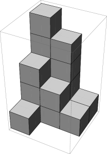
Figure 1. A plane partition of $n=17$

Definition 2.2.

A plane partition is totally symmetric iff whenever the position $(i,j,k)$ in its 3D Ferrers diagram is occupied (in other words $\pi_{ij}\geq k$), it follows that all its permutations $\{(i,k,j),(j,i,k),(j,k,i),(k,i,j),(k,j,i)\}$ are also occupied.

Now Stembridge’s theorem [8] can be easily stated:

Theorem 2.3.

The number of totally symmetric plane partitions whose 3D Ferrers diagram is contained in the cube $[0,n]^{3}$ is given by the nice product-formula

(2.1) $$\prod_{1\leq i\leq j\leq k\leq n}\frac{i+j+k-1}{i+j+k-2}.$$

Example 2.4.

We are considering the case $n=2$: Formula (2.1) tells us that there should be

$$\prod_{1\leq i\leq j\leq k\leq 2}\frac{i+j+k-1}{i+j+k-2}=\frac{2}{1}\cdot\frac{3}{2}\cdot\frac{4}{3}\cdot\frac{5}{4}=5$$

TSPPs inside the cube $[0,2]^{3}$ which is confirmed by the enumeration given in Figure 2.

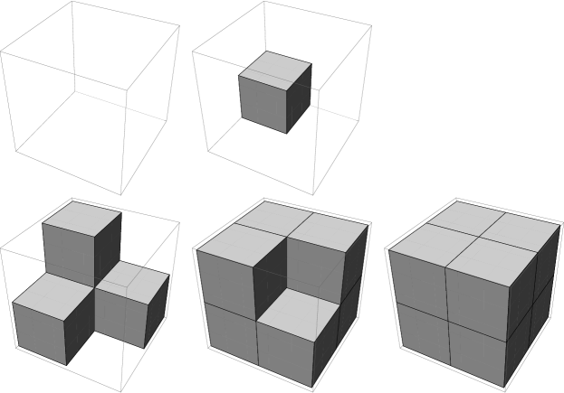
Figure 2. All TSPPs that fit into the cube $[0,2]^{2}$

As others that proved the TSPP formula before us we will make use of a result by Soichi Okada [7] that reduces the proof of Theorem 2.3 to a determinant evaluation:

Theorem 2.5.

The enumeration formula (2.1) for TSPPs is correct if and only if the determinant evaluation

(2.2) $$\det\,(a(i,j))_{1\leq i,j\leq n}=\prod_{1\leq i\leq j\leq k\leq n}\left(\frac{i+j+k-1}{i+j+k-2}\right)^{2}$$

holds, where the entries in the matrix are given by

(2.3) $$a(i,j)={i+j-2\choose i-1}+{i+j-1\choose i}+2\delta(i,j)-\delta(i,j+1).$$

In the above, $\delta(i,j)$ denotes the Kronecker delta.

Ten years after Stembridge’s proof, George Andrews, Peter Paule, and Carsten Schneider [1] came up with a computer-assisted proof. They transformed the problem into the task to verify a couple of hypergeometric multiple-sum identities (which they could do by the computer). This problem transformation however required human insight. We claim to have the first “human-free” computer proof of Stembridge’s theorem that is completely algorithmic and does not require any human insight into the problem. Moreover our method generalizes immediately to the $q$-case which is not so obvious to achieve in the approach presented in [1].

3. Proof method for determinant evaluations

Doron Zeilberger [13] proposes a method for completely automatic and rigorous proofs of determinant evaluations that fit into a certain class. For the sake of self-containedness this section gives a short summary how the method works. It addresses the problem: For all $n\geq 0$ prove that

$$\det(a(i,j))_{1\leq i,j\leq n}=\mathrm{Nice}(n),$$

for some explicitly given expressions $a(i,j)$ and $\mathrm{Nice}(n)$. What you have to do is the following: Pull out of the hat another discrete function $B(n,j)$ (this looks a little bit like magic for now—we will make this step more explicit in the next section) and check the identities

(3.1) $$\sum_{j=1}^{n}B(n,j)a(i,j) = 0\quad\mathrm{for\ }1\leq i<n,\quad i,n\in\mathbb{N},$$

(3.2) $$B(n,n) = 1\quad\mathrm{for\ all\ }n\geq 1,\quad n\in\mathbb{N}.$$

Then by uniqueness, it follows that $B(n,j)$ equals the cofactor of the $(n,j)$ entry of the $n\times n$ determinant (i.e. the minor with the last row and the $j$th column removed, this means we expand the determinant with respect to the last row using Laplace’s formula), divided by the $(n-1)\times(n-1)$ determinant. In other words we normalized in a way such that the last entry $B(n,n)$ is 1. Or, to make the argument even more explicit: What happens if we replace the last row of the matrix by any of the other rows? Clearly then the determinant will be zero; and nothing else is expressed in equation (3.1).

Finally one has to verify the identity

(3.3) $$\sum_{j=1}^{n}B(n,j)a(n,j)=\frac{\mathrm{Nice}(n)}{\mathrm{Nice}(n-1)}\quad\mathrm{for\ all\ }n\geq 1,\quad n\in\mathbb{N}.$$

If the suggested function $B(n,j)$ does satisfy all these identities then the determinant identity follows immediately as a consequence.

4. The algorithms

We now explain how the existing algorithms (in short) as well as our approach (in more detail) find a recurrence for some definite sum. In order to keep the descriptions simple and concrete we consider a sum of the form

$$\sum_{j=1}^{n}f(n,j)$$

as it appears in (3.3) (everything generalizes to instances with more parameters in the summand as it is the case in (3.1)). We give some indications why the existing algorithms fail to work in practice; all these statements refer to (3.3) but apply in a similar fashion to (3.1) as well.

4.1. Some unsuccessful tries

There are several methods in the literature how to algorithmically prove identities like (3.1) and (3.3). The first one traces back to Doron Zeilberger’s seminal paper [12] and he later named it the slow algorithm. The idea is to find a recurrence operator in the annihilating ideal of the summand that does not contain the summation variable in its coefficients; such a relation can always be rewritten in the form

$$P(n,S_{\!n})+(S_{\!j}-1)Q(n,S_{\!j},S_{\!n})$$

and we call $P$ the principal part and $Q$ the delta part. Such a telescoping relation encodes that $P$ is a recurrence for the sum (depending on the summand and the delta part we might have to add an inhomogeneous part to this recurrence). The elimination can be performed by a Gröbner basis computation with appropriate term order. In order to get a handle on the variable $j$ we have to consider the recurrences as polynomials in $j$, $S_{\!j}$, and $S_{\!n}$ with coefficients in $\mathbb{Q}(n)$ (for efficiency reasons this is preferable compared to viewing the recurrences as polynomials in all 4 indeterminates with coefficients in $\mathbb{Q}$). We tried this approach but it seems to be hopeless: The variable $j$ that we would like to eliminate occurs in the annihilating relations for the summand $B(n,j)a^{\prime}(n,j)$ with degrees between 24 and 30. When we follow the intermediate results of the Gröbner basis computation we observe that none of the elements that were added to the basis because some S-polynomial did not reduce to zero has a degree in $j$ lower than 23 (we aborted the computation after more than 48 hours). Additionally the coefficients grow rapidly and it seems very likely that we run out of memory before coming to an end.

The second option that we can try is often referred to as Takayama’s algorithm [9]. In fact, we would like to apply a variant of Takayama’s original algorithm that was proposed by Chyzak and Salvy [3]. Concerning speed this algorithm is much superior to the elimination algorithm described above: It computes only the principal part $P$ of some telescoping operator

(4.1) $$P(n,S_{\!n})+(S_{\!j}-1)Q(j,n,S_{\!j},S_{\!n}).$$

When we sum over natural boundaries we need not to know about the delta part $Q$. This is for example the case when the summand has only finite support (which is the case in our application). Also this algorithm boils down to an elimination problem which, as before, seems to be unsolvable with today’s computers: We now can lower the degree of $j$ to 18, but the intermediate results consume already about 12GB of memory (after 48 hours).

The third option is Chyzak’s algorithm [2] for $\partial$-finite functions: It finds a relation of the form (4.1) by making an ansatz for $P$ and $Q$; the input recurrences are interpreted as polynomials in $S_{\!j}$ and $S_{\!n}$ with coefficients being rational functions in $j$ and $n$. It uses the fact that the support of $Q$ can be restricted to the monomials under the stairs of the input annihilator and it loops over the order of $P$. Because of the multiplication of $Q$ by $S_{\!j}-1$ we end up in solving a coupled linear system of difference equations for the unknown coefficients of $Q$. Due to the size of the input, we did not succeed in uncoupling this system, and even if we can do this step, it remains to solve a presumably huge (concerning the size of the coefficients as well as the order) scalar difference equation.

4.2. A successful approach

The basic idea of what we propose is very simple: We also start with an ansatz in order to find a telescoping operator. But in contrast to Chyzak’s algorithm we avoid the expensive uncoupling and solving of difference equations. The difference is that we start with a polynomial ansatz in $j$ up to some degree:

(4.2) $$\underbrace{\sum_{i=0}^{I}c_{i}(n)S_{\!n}^{i}}_{=\>P(n,S_{\!n})}\quad+\quad(S_{\!j}-1)\cdot\underbrace{\sum_{k=0}^{K}\sum_{l=0}^{L}\sum_{m=0}^{M}d_{k,l,m}(n)j^{k}S_{\!j}^{l}S_{\!n}^{m}}_{=\>Q(j,n,S_{\!j},S_{\!n})}.$$

The unknown functions $c_{i}$ and $d_{k,l,m}$ to solve for are rational functions in $n$ and they can be computed using pure linear algebra. Recall that in Chyzak’s algorithm we have to solve for rational functions in $n$ and $j$ which causes the system to be coupled. The prize that we pay is that the shape of the ansatz is not at all clear from a priori: The order of the principal part, the degree bound for the variable $j$ and the support of the delta part need to be fixed, whereas in Chyzak’s algorithm we have to loop only over the order of the principal part. Our approach is similar to the generalization of Sister Celine Fasenmyer’s technique that is used in Wegschaider’s MultiSum package [11] (which can deal with multiple sums but only with hypergeometric summands). We proceed by reducing the ansatz with a Gröbner basis of the given annihilating left ideal for the summand, obtaining a normal form representation of the ansatz. Since we wish this relation to be in the ideal, the normal form has to be identically zero. Equating the coefficients of the normal form to zero and performing coefficient comparison with respect to $j$ delivers a linear system for the unknowns that has to be solved over $\mathbb{Q}(n)$.

Trying out for which choice of $I,K,L,M$ the ansatz delivers a solution can be a time-consuming tedious task. Additionally, once a solution is found it still can happen that it does not fit to our needs: It can well happen that all $c_{i}$ are zero in which case the result is useless. Hence the question is: Can we simplify the search for a good ansatz, for example, by using homomorphic images? Clearly we can reduce the size of the coefficients by computing modulo a prime number (we may assume that the input operators have coefficients in $\mathbb{Z}[j,n]$, otherwise we can clear denominators). But in practice this does not reduce the computational complexity too much—still we have bivariate polynomials that can grow dramatically during the reduction process. For sure we can not get rid of the variable $j$ since it is needed later for the coefficient comparison. It is also true that we can not just plug in some concrete integer for $n$: We would lose the feature of noncommutativity that $n$ shares with $S_{\!n}$ (recall that $S_{\!n}n=(n+1)S_{\!n}$, but $S_{\!n}7=7S_{\!n}$ for example). And the noncommutativity plays a crucial role during the reduction process, in the sense that omitting it we get a wrong result. Let’s have a closer look what happens and recall how the normal form computation works:

Algorithm: Normal form computation
Input: an operator $p$ and a Gröbner basis $G=\{g_{1},\dots,g_{m}\}$
Output: normal form of $p$ modulo the left ideal $\langle G\rangle$
while exists $1\leq i\leq m$ such that $\mathrm{lm}(g_{i})\,\mid\,\mathrm{lm}(p)$
	$g:=(\mathrm{lm}(p)/\mathrm{lm}(g_{i}))\cdot g_{i}$
	$p:=p-(\mathrm{lc}(p)/\mathrm{lc}(g))\cdot g$
end while
return $p$

where $\mathrm{lm}$ and $\mathrm{lc}$ refer to the leading monomial and the leading coefficient of an operator respectively.

Note that we do the multiplication of the polynomial that we want to reduce with in two steps: First multiply by the appropriate power product of shift operators (line 2), and second adjust the leading coefficient (line 3). The reason is because the first step usually will change the leading coefficient. Note also that $p$ is never multiplied by anything. This gives rise to a modular version of the normal form computation that does respect the noncommutativity.

Algorithm: Modular normal form computation
Input: an operator $p$ and a Gröbner basis $G=\{g_{1},\dots,g_{m}\}$
Output: modular normal form of $p$ modulo the left ideal $\langle G\rangle$
while exists $1\leq i\leq m$ such that $\mathrm{lm}(g_{i})\,\mid\,\mathrm{lm}(p)$
	$g:=h((\mathrm{lm}(p)/\mathrm{lm}(g_{i}))\cdot g_{i})$
	$p:=p-(\mathrm{lc}(p)/\mathrm{lc}(g))\cdot g$
end while
return $p$

where $h$ is an insertion homomorphism, in our example $h:\mathbb{Q}(j,n)\to\mathbb{Q}(j)$, $h(f(j,n))\mapsto f(j,n_{0})$ for some $n_{0}\in\mathbb{N}$. Thus most of the computations are done modulo the polynomial $n-n_{0}$ and the coefficient growth is moderate compared to before (univariate vs. bivariate).

Before starting the nonmodular computation we make the ansatz as small as possible by leaving away all unknowns that are 0 in the modular solution. With very high probability they will be 0 in the final solution too—in the opposite case we will realize this unlikely event since then the system will turn out to be unsolvable. In [11] a method called Verbaeten’s completion is used in order to recognize superfluous terms in the ansatz a priori. We were thinking about a generalization of that, but since the modular computation is negligibly short compared to the rest, we don’t expect to gain much and do not investigate this idea further.

Other optimizations concern the way how the reduction is performed. With a big ansatz that involves hundreds of unknowns (as it will be the case in our work) it is nearly impossible to do it in the naive way. The only possibility to achieve the result at reasonable cost is to consider each monomial in the support of the ansatz separately. After having computed the normal forms of all these monomials we can combine them in order to obtain the normal form of the ansatz. Last but not least it pays off to make use of the previously computed normal forms. This means that we sort the monomials that we would like to reduce according to the term order in which the Gröbner basis is given. Then for each monomial we have to perform one reduction step and then plug in the normal forms that we have already (since all monomials that occur in the support after the reduction step are smaller with respect to the chosen term order).

5. The computer proof

We are now going to give the details of our computer proof of Theorem 2.3 following the lines described in the previous section.

5.1. Get an annihilating ideal

The first thing we have to do according to Zeilberger’s algorithmic proof technique is to resolve the magic step that we have left as a black box so far, namely “to pull out of the hat” the sequence $B(n,j)$ for which we have to verify the identities (3.1) – (3.3). Note that we are able, using the definition of what $B(n,j)$ is supposed to be (namely a certain minor in a determinant expansion), to compute the values of $B(n,j)$ for small concrete integers $n$ and $j$. This data allows us (by plugging it into an appropriate ansatz and solving the resulting linear system of equations) to find recurrence relations for $B(n,j)$ that will hold for all values of $n$ and $j$ with a very high probability. We call this method guessing; it has been executed by Manuel Kauers who used his highly optimized software Guess.m [4]. More details about this part of the proof can be found in [5]. The result of the guessing were 65 recurrences, their total size being about 5MB.

Many of these recurrences are redundant and it is desirable to have a unique description of the object in question that additionally is as small as possible (in a certain metric). To this end we compute a Gröbner basis of the left ideal that is generated by the 65 recurrences. The computation was executed by the author’s noncommutative Gröbner basis implementation which is part of the package HolonomicFunctions. The Gröbner basis consists of 5 polynomials (their total size being about 1.6MB). Their leading monomials $S_{\!j}^{4},S_{\!j}^{3}S_{\!n},S_{\!j}^{2}S_{\!n}^{2},S_{\!j}S_{\!n}^{3},S_{\!n}^{4}$ form a staircase of regular shape. This means that we should take 10 initial values into account (they correspond to the monomials under the staircase).

In addition, we have now verified that all the 65 recurrences are consistent. Hence they are all describing the same object. But since we want to have a rigorous proof we have to admit at this point that what we have found so far (that is a $\partial$-finite description of some bivariate sequence—let’s call it $B^{\prime}(n,j)$) does not prove anything yet. We have to show that this $B^{\prime}(n,j)$ is identical to the sequence $B(n,j)$ defined by (3.1) and (3.2). Finally we have to show that identity (3.3) indeed holds.

5.2. Avoid singularities

Before we start to prove the relevant identities there is one subtle point that, aiming at a fully rigorous proof, we should not omit: the question of singularities in the $\partial$-finite description of $B^{\prime}(n,j)$. Recall that in the univariate case when we deal with a P-finite recurrence, we have to regard the zeros of the leading coefficient and in case that they introduce singularities in the range where we would like to apply the recurrence, we have to separately specify the values of the sequence at these points. Similarly in the bivariate case: We have to check whether there are points in $\mathbb{N}^{2}$ where none of the recurrences can be applied because the leading term vanishes. For all points that lie in the area $(4,4)+\mathbb{N}^{2}$ we may apply any of the recurrences, hence we have to look for common nonnegative integer solutions of all their leading coefficients. A Gröbner basis computation reveals that everything goes well: From the first element of the Gröbner basis

$$(n-3)^{2}(n-2)(n-1)^{2}(2n-3)^{2}(2n-1)(j+n-1)(j+n)$$

we can read off the solutions $(0,0)$, $(1,0)$, and $(0,1)$ (which are also solutions of the remaining polynomials but since they are lying under the stairs they are of no interest). Further we have to address the cases $n=1,2,3$. Plugging these into the remaining polynomials we obtain further common solutions: $(1,1)$, $(2,1)$, $(2,2)$, $(3,2)$, and $(3,3)$. But all of them are outside of $(4,4)+\mathbb{N}^{2}$ so we need not to care. It remains to look at the lines $j=0,1,2,3$ and the lines $n=0,1,2,3$ (we omit the details here). Summarizing, the points for which initial values have to be given (either because they are under the stairs or because of singularities) are

$$\begin{array}[]{l}\{(j,n)\mid 0\leq j\leq 6\land 0\leq n\leq 1\}\cup\{(j,2)\mid 0\leq j\leq 4\}\cup\{(j,3)\mid 0\leq j\leq 3\}\cup\\ \{(j,4)\mid 0\leq j\leq 2\}\cup\{(1,5)\}.\end{array}$$

They are depicted in Figure 3.

Figure 3. The points for which the initial values of the sequence $B(n,j)$ have to be given because the recurrences do not apply.

5.3. The second identity

The simplest of the three identities to prove is (3.2). From the $\partial$-finite description of $B^{\prime}(n,j)$ we can compute a recurrence for the diagonal $B^{\prime}(n,n)$ by the closure property “substitution”. HolonomicFunctions delivers a recurrence of order 7 in a couple of minutes. Reducing this recurrence with the ideal generated by $S_{\!n}-1$ (which annihilates 1) gives 0; hence it is a left multiple of the recurrence for the right hand side. We should not forget to have a look on the leading coefficient in order to make sure that we don’t run into singularities:

$$256(2n+3)(2n+5)(2n+7)(2n+9)(2n+11)^{2}(2n+13)^{2}p_{1}p_{2}$$

where $p_{1}$ and $p_{2}$ are irreducible polynomials in $n$ of degree 4 and 12 respectively. Comparing initial values (which of course match due to our definition) establishes identity (3.2).

5.4. The third identity

In order to prove (3.3) we first rewrite it slightly. Using the definition of the matrix entries $a(n,j)$ we obtain for the left hand side

$$\sum_{j=1}^{n}B(n,j)\underbrace{\left({n+j-2\choose n-1}+{n+j-1\choose n}\right)}_{=:a^{\prime}(n,j)}\>+2B(n,n)-B(n,n-1)$$

and the right hand side simplifies to

$$\frac{\mathrm{Nice}(n)}{\mathrm{Nice}(n-1)}=\frac{\prod_{1\leq i\leq j\leq k\leq n}\left(\frac{i+j+k-1}{i+j+k-2}\right)^{2}}{\prod_{1\leq i\leq j\leq k\leq n-1}\left(\frac{i+j+k-1}{i+j+k-2}\right)^{2}}=\frac{4^{1-n}(3n-1)^{2}(2n)_{n-1}^{2}}{(3n-2)^{2}(n/2)_{n-1}^{2}}.$$

Note that $a^{\prime}(n,j)=\frac{2n+j-1}{n+j-1}{n+j-1\choose j-1}$ is a hypergeometric expression in both variables $j$ and $n$. A $\partial$-finite description of the summand can be computed with HolonomicFunctions from the annihilator of $B(n,j)$ by closure property. We found by means of modular computations that the ansatz (4.2) with $I=7$, $K=5$, and the support of $Q$ being the power products $S_{\!j}^{l}S_{\!n}^{m}$ with $l+m\leq 7$ delivers a solution with nontrivial principal part. After omitting the 0-components of this solution, we ended up with an ansatz containing 126 unknowns. For computing the final solution we used again homomorphic images and rational reconstruction. Still it was quite some effort to compute the solution (it consists of rational functions in $n$ with degrees up to 382 in the numerators and denominators). The total size of the telescoping relation becomes smaller when we reduce the delta part to normal form (then obtaining an operator of the form that Chyzak’s algorithm delivers). Finally the result takes about 5 MB of memory. We counterchecked its correctness by reducing the relation with the annihilator of $B(n,j)a^{\prime}(n,j)$ and obtained 0 as expected.

We have now a recurrence for the sum but we need to to cover the whole left hand side. A recurrence for $B(n,n-1)$ is easily obtained with our package performing the substitution $j\to n-1$, and $B(n,n)=1$ as shown before. The closure property “sum of $\partial$-finite functions” delivers a recurrence of order 10. On the right hand side we have a $\partial$-finite expression for which our package automatically computes an annihilating operator. This operator is a right divisor of the one that annihilates the left hand side. By comparing 10 initial values and verifying that the leading coefficients of the recurrences do not have singularities among the positive integers, we have established identity (3.3).

5.5. The first identity

With the same notation as before we reformulate identity (3.1) as

$$\sum_{j=1}^{n}B(n,j)a^{\prime}(i,j)=B(n,i-1)-2B(n,i).$$

The hard part again is to do the sum on the left hand side. Since two parameters $i$ and $n$ are involved and remain after the summation, one annihilating operator does not suffice. We decided to search for two operators with leading monomials being pure powers of $S_{\!i}$ and $S_{\!n}$ respectively. Although this is far away from being a Gröbner basis, it is nevertheless a complete description of the object (together with sufficiently (but still finitely) many initial values). We obtained these two relations in a similar way as in the previous section, but the computational effort was even bigger (more than 500 hours of computation time were needed). The first telescoping operator is about 200 MB big and the support of its principal part is

$$\begin{array}[]{ll}\{&S_{\!i}^{5},S_{\!i}^{4}S_{\!n},S_{\!i}^{3}S_{\!n}^{2},S_{\!i}^{2}S_{\!n}^{3},S_{\!i}S_{\!n}^{4},S_{\!i}^{4},S_{\!i}^{3}S_{\!n},S_{\!i}^{2}S_{\!n}^{2},S_{\!i}S_{\!n}^{3},\\ &S_{\!i}^{3},S_{\!i}^{2}S_{\!n},S_{\!i}S_{\!n}^{2},S_{\!n}^{3},S_{\!i}^{2},S_{\!i}S_{\!n},S_{\!n}^{2},S_{\!i},S_{\!n},1\}.\end{array}$$

The second one is of size 700 MB and the support of its principal part is

$$\{S_{\!n}^{5},S_{\!i}^{4},S_{\!i}^{3}S_{\!n},S_{\!i}^{2}S_{\!n}^{2},S_{\!i}S_{\!n}^{3},S_{\!n}^{4},S_{\!i}^{3},S_{\!i}^{2}S_{\!n},S_{\!i}S_{\!n}^{2},S_{\!n}^{3},S_{\!i}^{2},S_{\!i}S_{\!n},S_{\!n}^{2},S_{\!i},S_{\!n},1\}.$$

Again we can independently from their derivation check their correctness by reducing them with the annihilator of $B(n,j)a^{\prime}(i,j)$: both give 0.

Let’s now address the right hand side: From the Gröbner basis for $B(n,j)$ that we computed in Section 5.1 one immediately gets the annihilator for $B(n,i-1)$ by replacing $S_{\!j}$ by $S_{\!i}$ and by substituting $j\to i-1$ in the coefficients. We now could apply the closure property “sum of $\partial$-finite functions” but we can do better: Since the right hand side can be written as $(1-2S_{\!i})\bullet B(n,i-1)$ we can use the closure property “application of an operator” and obtain a Gröbner basis which has even less monomials under the stairs than the input, namely 8. The opposite we expect to happen when using “sum”: usually there the dimension grows but never can shrink. It is now a relatively simple task to verify that the two principal parts that were computed for the left hand side are elements of the annihilating ideal of the right hand side (both reductions give 0).

The initial value question needs some special attention here since we want the identity to hold only for $i<n$; hence we can not simply look at the initial values in the square $[0,4]^{2}$. Instead we compare the initial values in a trapezoid-shaped area which allows us to compute all values below the diagonal. Since all these initial values match for the left hand and right hand side we have the proof that the identity holds for all $i<n$. Looking at the leading coefficients of the two principal parts we find that they contain the factors $5+i-n$ and $5-i+n$ respectively. This means that both operators can not be used to compute values on the diagonal which is a strong indication that the identity does not hold there: Indeed, identity (3.1) is wrong for $n=i$ because in this case we get (3.3).

6. Outlook

As we have demonstrated Zeilberger’s methodology is completely algorithmic and does not need human intervention. This fact makes it possible to apply it to other problems (of the same class) without further thinking. Just feed the data into the computer! The $q$-TSPP enumeration formula

$$\prod_{1\leq i\leq j\leq k\leq n}\frac{1-q^{i+j+k-1}}{1-q^{i+j+k-2}}$$

has been conjectured independently by George Andrews and Dave Robbins in the early 1980s. This conjecture is still open and one of the most intriguing problems in enumerative combinatorics. The method as well as our improvements can be applied one-to-one to that problem (also a $q$-analogue of Okada’s result exists). Unfortunately, due to the additional indeterminate $q$ the complexity of the computations is increased considerably which prevents us from proving it right away. But we are working on that…

Acknowledgements. I would like to thank Doron Zeilberger for attentively following my efforts and providing me with helpful hints. Furthermore he was the person who came up with the idea to attack TSPP in the way we did. Special thanks go to my colleague Manuel Kauers with whom I had lots of fruitful discussions during this work and who performed the guessing part in Section 5.1. He also provided me with his valuable knowledge and software on how to efficiently solve linear systems using homomorphic images.

References

- [1] George E. Andrews, Peter Paule, and Carsten Schneider, Plane Partitions VI. Stembridge’s TSPP theorem, Adv. Appl. Math. 34 (2005), 709–739.
- [2] Frédéric Chyzak, An extension of zeilberger’s fast algorithm to general holonomic functions, Discrete Mathematics 217 (2000), no. 1-3, 115–134.
- [3] Frédéric Chyzak and Bruno Salvy, Non-commutative elimination in ore algebras proves multivariate identities, Journal of Symbolic Computation 26 (1998), 187–227.
- [4] Manuel Kauers, Guessing handbook, Tech. Report 09-07, RISC Report Series, University of Linz, Austria, 2009.
- [5] Manuel Kauers, Christoph Koutschan, and Doron Zeilberger, A proof of George Andrews’ and Dave Robbins’ q-TSPP conjecture (modulo a finite amount of routine calculations), The personal journal of Shalosh B. Ekhad and Doron Zeilberger (2009), 1–8, http://www.math.rutgers.edu/~zeilberg/pj.html.
- [6] Christoph Koutschan, Computer algebra algorithms for -finite and holonomic functions, Ph.D. thesis, RISC-Linz, 2009, in preparation.
- [7] Soichi Okada, On the generating functions for certain classes of plane partitions, Journal of Combinatorial Theory, Series A 53 (1989), 1–23.
- [8] John Stembridge, The enumeration of totally symmetric plane partitions, Advances in Mathematics 111 (1995), 227–243.
- [9] Nobuki Takayama, An algorithm of constructing the integral of a module–an infinite dimensional analog of Gröbner basis, ISSAC ’90: Proceedings of the international symposium on Symbolic and algebraic computation (New York, NY, USA), ACM, 1990, pp. 206–211.
- [10] by same author, Gröbner basis, integration and transcendental functions, ISSAC ’90: Proceedings of the international symposium on Symbolic and algebraic computation (New York, NY, USA), ACM, 1990, pp. 152–156.
- [11] Kurt Wegschaider, Computer generated proofs of binomial multi-sum identities, Master’s thesis, RISC, Johannes Kepler University Linz, May 1997.
- [12] Doron Zeilberger, A holonomic systems approach to special function identities, Journal of Computational and Applied Mathematics 32 (1990), no. 3, 321–368.
- [13] by same author, The HOLONOMIC ANSATZ II. Automatic DISCOVERY(!) and PROOF(!!) of Holonomic Determinant Evaluations, Annals of Combinatorics 11 (2007), 241–247.