Analytical Wake Potentials in a Closed Pillbox Cavity

Abstract

Wake potentials are derived for a closed (cylindrical) pillbox cavity as a sum over cavity modes. The resulting expression applies to on- and off-axis beams and test particles. The sum is evaluated numerically for a Gaussian drive bunch and compared to the wake potential derived from simulation.

I Introduction

The wake potential Bane et al. (1984); Wilson (1989) describes the interaction between two charged particles mitigated by an external structure; the wake potential is especially useful for considering charged particles traveling at relativistic speeds on parallel paths through structures (such as radio-frequency accelerating cavities) in a particle accelerator. In this paper we derive the longitudinal wake potential for highly relativistic beams traveling parallel to the axis—but not necessarily on the axis—of a closed (cylindrical) pillbox cavity.

The monopole wake potential for on-axis beams in a closed pillbox cavity was derived in Weiland and Zotter (1981) (see also Bane et al. (1984); Wilson (1989)). Analytical wake potentials have also been found for other geometries, such as closed spherical cavities Ratschow and Weiland (2002), conical cavities Tsakanian (2005), multi-cell pillbox cavities with elliptical cross section (for axial beams only) Kim et al. (1990), and multi-cell pillbox cavities with beam tubes Gao (1995, 1996). We note that the wake potential for a pillbox cavity with infinitely long beam tubes differs significantly from the wake potential in a closed pillbox cavity: in a pillbox cavity with infinitely long beam tubes, the parts of the wake potential that vary azimuthally as $\cos(m\theta)$ vary radially as $r^{m}$; in a closed pillbox cavity, the radial dependence is more complicated.

II Wake potential

The wake potential describes the momentum change of a test particle caused by the fields excited by another charged particle. When a point charge $q_{b}$ ($b$ for “beam”) travels through a cavity, it creates an electric field $\mathbf{E}(r,\theta,z,t)$ and also a magnetic field; the wake potential describes the momentum change of a test charge due to those fields.

The wake potential is particularly useful when applied to highly relativistic particles, which maintain nearly constant speed while changing momentum. If a charge $q_{b}$ travels at light speed along the path $(r,\theta,z)(t)=(r_{b},\theta_{b},ct)$, creating an electric field with $z$-component $E_{z}(r,\theta,z,t)$, its longitudinal wake potential is:

$$W_{z}(s;r_{b},\theta_{b},r_{t},\theta_{t})\equiv-\frac{1}{q_{b}}\int dz\,E_{z}(r_{t},\theta_{t},z,t\!=\!(z+s)/c).$$ (1)

(We will consider a closed cavity of length $\ell$, so the integration runs from $z=0$ to $z=\ell$.) If a test charge $q_{t}$ trails $q_{b}$ by a distance $s$, traveling along a parallel path $(r,\theta,z)(t)=(r_{t},\theta_{t},ct+s)$ from $z=0$ to $z=\ell$, its longitudinal momentum change due to the fields created by $q_{b}$ is

$$\Delta p_{z}(s;r_{t},\theta_{t})=-\frac{q_{t}q_{b}}{c}W_{z}(s;r_{b},\theta_{b},r_{t},\theta_{t})$$ (2)

(the test charge is assumed to be highly relativistic, so its speed remains constant even as its momentum changes). By convention, positive $W_{z}$ corresponds to a loss in momentum.

In cylindrically symmetric structures, it is helpful to decompose wakefields into azimuthal harmonics, i.e., fields with dependence $\cos(m\theta)$ and $\sin(m\theta)$ for $m=0,1,\ldots$:

$$W_{z}(s;r_{b},r_{t},\theta_{t})=\sum_{m=0}^{\infty}W_{z,m}(s;r_{b},r_{t})\cos(m\theta_{t})$$ (3)

where we have chosen the beam to be at $\theta_{b}=0$; symmetry prohibits the excitation of any modes with $\sin(m\theta)$ dependence. In structures with cylindrical symmetry and infinitely extended beam tubes, the azimuthal components of the wakefield have a particularly simple dependence on $r_{b}$ and $r_{t}$ (when they are smaller than the beam tube radius) Weiland (1983)

$$W_{z,m}(s;r_{b},r_{t})\propto r_{b}^{m}r_{t}^{m}.$$ (4)

However, Ref. Napoly et al. (1993) shows that this simple form depends on the fields at $z=\pm\infty$ being the fields of a charge in an infinitely long beam tube; in a closed cavity, the fields at the ends of integration (at $z=0$ and $z=\ell$) upset the simple dependence on $r_{b}$ and $r_{t}$, though $W_{z,m}$ still approximately assumes the above form for $r_{b}$ and $r_{t}$ near the axis.

III Pillbox Wake Potential

The monopole wake potential for a closed pillbox cavity has been derived for axial beam and test particles in Weiland and Zotter (1981). In the same way, we derive an analytical expression for multipole wakes, for beam and test particles following paths parallel to the axis. We will write the wake potential as a sum over cavity modes; only TM modes (with magnetic field transverse to the $z$ direction) will be excited, since the beam travels in the $z$ direction and TE modes have $E_{z}=0$. Choosing the beam to be at $\theta_{b}=0$, only TM modes with $\cos(m\theta)$ dependence will be excited, and we need not consider modes with $\sin(m\theta)$ dependence.

We can write the field in the pillbox cavity of radius $R$ and length $\ell$ as a sum over modes; the (cosine) mode $\textrm{TM}_{mnp}$ (for integers $m\geq 0$, $n\geq 1$, $p\geq 0$) has fields (see Chao and Tigner (1999), Sec. 7.3.7):

$$E_{z,mnp}(r,\theta,z,t) = \cos\left(\frac{p\pi z}{\ell}\right)J_{m}\left(\frac{j_{m,n}r}{R}\right)\cos(m\theta)e^{-i\omega_{mnp}t}$$ (5)

$$E_{r,mnp}(r,\theta,z,t) = -\left(\frac{p\pi}{\ell}\right)\frac{R}{j_{m,n}}\sin\left(\frac{p\pi z}{\ell}\right)J^{\prime}_{m}\left(\frac{j_{m,n}r}{R}\right)\cos(m\theta)e^{-i\omega_{mnp}t}$$ (6)

$$E_{\theta,mnp}(r,\theta,z,t) = \left(\frac{p\pi}{\ell}\right)\frac{R^{2}}{j_{m,n}^{2}}\sin\left(\frac{p\pi z}{\ell}\right)\frac{m}{r}J_{m}\left(\frac{j_{m,n}r}{R}\right)\sin(m\theta)e^{-i\omega_{mnp}t}$$ (7)

$$H_{r,mnp}(r,\theta,z,t) = i\sqrt{\frac{\epsilon_{0}}{\mu_{0}}}\frac{\omega_{mnp}R^{2}}{cj_{m,n}^{2}}\cos\left(\frac{p\pi z}{\ell}\right)\frac{m}{r}J_{m}\left(\frac{j_{m,n}r}{R}\right)\sin(m\theta)e^{-i\omega_{mnp}t}$$ (8)

$$H_{\theta,mnp}(r,\theta,z,t) = i\sqrt{\frac{\epsilon_{0}}{\mu_{0}}}\frac{\omega_{mnp}R}{cj_{m,n}}\cos\left(\frac{p\pi z}{\ell}\right)J^{\prime}_{m}\left(\frac{j_{m,n}r}{R}\right)\cos(m\theta)e^{-i\omega_{mnp}t}$$ (9)

where $J_{m}$ is the Bessel function of order $m$, $J_{m}^{\prime}$ is its derivative, and $j_{m,n}$ is the $n^{\textrm{th}}$ zero of $J_{m}$. Mode $\textrm{TM}_{mnp}$ oscillates with frequency $\omega_{mnp}$:

$$\frac{\omega_{mnp}^{2}}{c^{2}}=\frac{j_{m,n}^{2}}{R^{2}}+\left(\frac{p\pi}{\ell}\right)^{2}.$$ (10)

The wake potential for a highly relativistic point charge traveling parallel to the $z$ axis, at radius $r_{b}$ (and $\theta_{b}=0$), is Wilson (1989):

$$W_{z}(s;r_{b},r_{t},\theta_{t})=2H(s)\sum_{mnp}k_{mnp}(r_{b},r_{t},\theta_{t})\cos\left(\frac{\omega_{mnp}s}{c}\right)$$ (11)

where $H(s)$ is the Heaviside step function, and $H(0)=1/2$, and $k_{mnp}(r_{b},r_{t},\theta_{t})$ is the loss factor for mode $\textrm{TM}_{mnp}$:

$$k_{mnp}(r_{b},r_{t},\theta_{t})=\frac{V_{mnp}^{*}(r_{b},\theta_{b}=0)V_{mnp}(r_{t},\theta_{t})}{4U_{mnp}}$$ (12)

where $V_{mnp}(r,\theta)$ is the (complex) voltage gain of a test particle crossing the cavity at transverse position $(r,\theta)$, due to mode $\textrm{TM}_{mnp}$ when the cavity has stored energy $U_{mnp}$ in that mode:

$$V_{mnp}(r,\theta)=\int_{0}^{\ell}dz\,E(r,\theta,z,t=z/c)$$ (13)

$$=J_{m}\left(\frac{j_{m,n}r}{R}\right)\cos(m\theta)\frac{i\omega_{mnp}R^{2}}{cj_{m,n}^{2}}\left[(-1)^{p}e^{-i\omega_{mnp}\ell/c}-1\right]$$

and

$$U_{mnp} = \frac{1+\delta_{m0}}{2-\delta_{p0}}\frac{\pi\epsilon_{0}R^{4}\ell}{4j_{m,n}^{2}}J^{\prime}_{m}(j_{m,n})^{2}\frac{\omega_{mnp}^{2}}{c^{2}}$$ (14)

where $\delta_{mn}$ is the Kronecker delta. The loss factor is then:

$$k_{mnp}(r_{b},r_{t},\theta_{t}) = \frac{2-\delta_{p0}}{1+\delta_{m0}}\frac{J_{m}\left(\frac{j_{m,n}r_{b}}{R}\right)J_{m}\left(\frac{j_{m,n}r_{t}}{R}\right)\cos(m\theta_{t})\cdot 2\left[1-(-1)^{p}\cos(\omega_{mnp}\ell/c)\right]}{\displaystyle\pi\epsilon_{0}\ell j_{m,n}^{2}J^{\prime}_{m}(j_{m,n})^{2}}.$$ (15)

The sum in Eq. (11) unfortunately does not converge: for fixed $m$ and $n$, the terms oscillate with constant amplitude as $p$ increases. In case the beam and test particles travel along the same line, the sum can be analytically evaluated for $s$ small enough that the walls at $r=R$ can have no effect Weiland and Zotter (1981); Wilson (1989)—it sums to a sequence of delta functions, which offers some explanation for the sum’s lack of convergence (considering the representation of a delta function as a non-convergent Fourier series).

The sum’s behavior can be improved by calculating the wake potential due to a charged bunch with total charge $q_{b}$ and linear density profile $\lambda(s)$, rather than a point charge. The bunch wake potential is

$$V_{z}(s)=\int_{0}^{\infty}ds^{\prime}\lambda(s-s^{\prime})W_{z}(s^{\prime}).$$ (16)

We will consider a Gaussian bunch

$$\lambda(s)=\frac{1}{\sqrt{2\pi}\sigma}\exp\left(-\frac{s^{2}}{2\sigma^{2}}\right)$$ (17)

and replace the $\cos(\omega_{mnp}s/c)$ term in Eq. (11), with the integral

$$\int_{0}^{\infty}ds^{\prime}\,\frac{1}{\sqrt{2\pi}\sigma}\exp\left(-\frac{(s-s^{\prime})^{2}}{2\sigma^{2}}\right)\cos(ks^{\prime})$$

$$=\frac{1}{2}\exp\left(-\frac{\sigma^{2}k^{2}}{2}\right)\textrm{Re}\left[e^{iks}\textrm{erfc}\left(-\frac{s+i\sigma^{2}k}{\sqrt{2}\sigma}\right)\right],$$ (18)

where $k=\omega_{mnp}/c$, and erfc is one minus the error function (of a complex argument). The bunch wake potential is:

$$V_{z}(s;r_{b},r_{t},\theta_{t}) = 2H(s)\sum_{m,n,p}\frac{2-\delta_{p0}}{1+\delta_{m0}}$$ (19)

$$\times\frac{J_{m}\left(\frac{j_{m,n}r_{b}}{R}\right)J_{m}\left(\frac{j_{m,n}r_{t}}{R}\right)\cos(m\theta_{t})\cdot 2\left[1-(-1)^{p}\cos(\omega_{mnp}\ell/c)\right]}{\displaystyle\pi\epsilon_{0}\ell j_{m,n}^{2}J^{\prime}_{m}(j_{m,n})^{2}}$$

$$\times\frac{1}{2}\exp\left(-\frac{\sigma^{2}\omega_{mnp}^{2}}{2c^{2}}\right)\textrm{Re}\left[e^{i\omega_{mnp}s/c}\textrm{erfc}\left(-\frac{s+i\sigma^{2}\omega_{mnp}/c}{\sqrt{2}\sigma}\right)\right].$$

If we wish to know just the contribution from modes with $\cos(m\theta)$ dependence, we sum only over modes with that $m$.

For $x\ll m$, $J_{m}(x)\approx(x/2)^{m}/m!$ Abramowitz and Stegun (1972), so the multipole contributions to the wake are proportional to $r_{t}^{m}r_{b}^{m}$ when $r_{b}^{m}$ and $r_{t}^{m}$ are small.

IV Numerical Pitfalls

The bunch potential in Eq. (19) can be evaluated in a straightforward manner, except for the function $e^{-y^{2}+2ixy}\textrm{erfc}(-x-iy)$, where we have used the abbreviations $x=s/(\sqrt{2}\sigma)$ and $y=\sigma\omega_{mnp}/(\sqrt{2}c)$.

An easy and fast way to evaluate erfc uses the Faddeeva function $w(z)\equiv e^{-z^{2}}\textrm{erfc}(-iz)$ computed by the method of Weideman (1994); i.e.,

$$e^{-y^{2}+2ixy}\textrm{erfc}(-x-iy)=e^{-x^{2}}w(y-ix).$$ (20)

However, $w(y-ix)$ becomes enormous for $x^{2}\gg y^{2}$, while $e^{-x^{2}}w(y-ix)$ remains tractable; similarly, for large $y^{2}$, $\textrm{erfc}(-x-iy)$ is enormous. In these cases we use the asymptotic expansion for erfc (see Abramowitz and Stegun (1972)); because the expansion in Abramowitz and Stegun (1972) for $\textrm{erfc}(z)$ is valid for $|\textrm{arg}z|<3\pi/4$, we have to apply the identity $\textrm{erfc}(-x-iy)=2-\textrm{erfc}(x+iy)$ before using the expansion when $x>|y|$.

Specifically, to prevent overflow with double precision arithmetic, we perform a different evaluation for the following cases: if $x^{2}-y^{2}>500$ and $x>0$, we evaluate

$$e^{-y^{2}+2ixy}\textrm{erfc}(-x-iy)\approx 2e^{-y^{2}+2ixy}$$ (21)

and if $x^{2}-y^{2}>500$ and $x<0$, or if $y^{2}-x^{2}>500$, then we evaluate

$$e^{-y^{2}+2ixy}\textrm{erfc}(-x-iy)\approx-\frac{e^{-x^{2}}}{\sqrt{\pi}(x+iy)}\left[1+\sum_{m=1}^{6}(-1)^{m}\frac{1\cdot 3\ldots(2m-1)}{[2(x^{2}-y^{2}+2ixy)]^{m}}\right].$$ (22)

These approximations yield nearly full accuracy in double precision when the specified conditions are satisfied.

V Behavior for large $n$ and $p$

In this section we show the behavior of terms in the sum in Eq. (19) for large $n$ and $p$. For large $p$ ($\omega_{mnp}/c\gg 1/\sigma$), we must consider two cases (the asymptotic limits are given in Sec. IV): the non-oscillatory contributions that depend on $p$ behave as

$$\exp\left(-\frac{\sigma^{2}\omega_{mnp}^{2}}{2c^{2}}\right)\textrm{Re}\left[e^{i\omega_{mnp}s/c}\textrm{erfc}\left(-\frac{s+i\sigma^{2}\omega_{mnp}/c}{\sqrt{2}\sigma}\right)\right]$$

$$\sim\left\{\begin{array}[]{c@{\quad}l}2e^{-\sigma^{2}(\omega_{mnp}/c)^{2}/2}\cos(\omega_{mnp}s/c)&\textrm{ if }s/\sigma\gg\sigma\omega_{mnp}/c\\ -\sqrt{\frac{2}{\pi}}\frac{s/\sigma}{(s/\sigma)^{2}+(\sigma\omega_{mnp}/c)^{2}}e^{-s^{2}/2\sigma^{2}}&\textrm{ if }|s/\sigma|\ll\sigma\omega_{mnp}/c\end{array}\right.$$ (25)

When $s\gg\sigma$, convergence is very fast (with truncation error falling as the tail of a Gaussian), since the Gaussian charge distribution has had time to cancel out high-frequency contributions. When $s$ is comparable to or smaller than $\sigma$, the wake potential “feels” only part of the charge distribution, and higher frequencies matter more; consequently, the terms in the sum eventually fall off as $1/\omega_{mnp}^{2}$.

For fixed $m$, but large $n$ ($n\gg mR/r_{b}$, $n\gg mR/r_{t}$), the envelope behavior (ignoring oscillatory contributions) of terms in the bunch potential series that depend on $n$ is:

$$\frac{J_{m}\left(\frac{j_{m,n}r_{b}}{R}\right)J_{m}\left(\frac{j_{m,n}r_{t}}{R}\right)}{\displaystyle j_{m,n}^{2}J^{\prime}_{m}(j_{m,n})^{2}}\sim\frac{R}{(n+m/2)^{2}\pi^{2}\sqrt{r_{b}r_{t}}},$$ (26)

decreasing slowly as $\sim 1/n^{2}$.

VI Wake potential simulation

We compared the analytical wake potential against $W_{z,m}(s;r_{b},r_{t})$ calculated via simulation, using the electromagnetic particle-in-cell (PIC) simulation capability of vorpal Nieter and Cary (2004) in Cartesian coordinates. We excited a cavity using a current bunch at $r_{b}$ (and $\theta_{b}=0$), with a Gaussian width $\sigma$ in the longitudinal direction $z$; the current bunch traveled at a highly relativistic speed and was (artificially) unaffected by the fields it generated. At each time step, we injected highly relativistic test particles (with charges too small to affect the cavity fields) at radius $r_{t}$ and regularly-spaced angles $\theta_{t}$, and recorded the momentum change of each test particle after crossing the cavity. We thus measured $\Delta p_{z}(s;r_{t},\theta_{t})$, which, after decomposition into azimuthal harmonics, yielded $W_{z,m}(s;r_{b},r_{t})$.

With a radius $R=11.5\>$mm, the cavity’s $\textrm{TM}_{010}$ mode oscillated at 10 GHz; the length was chosen to be one-half wavelength at that frequency, $\ell=15.0\>$mm. The Gaussian bunch [as in Eq. (16)] had $\sigma=2\ell/25$ (but was very thin in cross-section). Following the advice of Ref. Chao and Tigner (1999) (Sec. 3.2.3), we chose the cell length $\Delta z<\sqrt{\sigma^{3}/\ell}$, resulting in $\Delta z=0.333\>$mm and transverse cell sizes $\Delta x=\Delta y=0.336\>$mm.

The curved metal boundaries of the cavity were simulated using the Dey-Mittra algorithm Dey and Mittra (1999), which requires (for improved accuracy) a reduction in time step from the standard Courant-Friedrichs-Lewy time step.

(a)
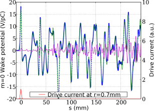
(b)

Figure 1: Monopole wake potential (a) and dipole wake potential divided by the test-particle radius (b) in the closed pillbox cavity: the analytical (green line) and simulated (blue circles) wake potentials are nearly the same; the difference between them is shown by the magenta line; the red line at the bottom shows the drive current. The analytical sum was cutoff above $\omega/c=300/\sigma$ ($f\approx 1.2\times 10^{4}\>$GHz) for $s/\sigma<8.5$ and $\omega/c=10/\sigma$ ($400\>$GHz) for larger $s$. Simulated results are shown for cells of size $0.33\>$mm, and a time step half the Courant-Friedrichs-Lewy time step.

Figure 1 shows the resulting $m=0$ and $m=1$ components of the wake (bunch) potential for identical beam and test-particle radii, $r_{b}=r_{t}=0.672\>$mm. The difference between the analytical and simulated wakefield grows in time as the simulated modes slip in phase with respect to the analytical modes (due to error in the frequency of the simulated modes).

(a)
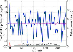
(b)

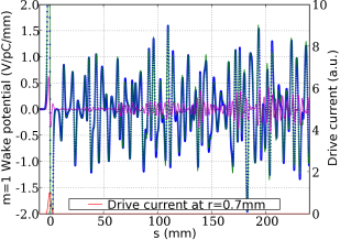
Figure 2: Monopole wake potential (a) and dipole wake potential divided by the test-particle radius (b) in the closed pillbox cavity: the analytical (green line) and simulated (blue circles) wake potentials are nearly the same; the difference between them is shown by the magenta line. The analytical sum was cutoff above $\omega/c=300/\sigma$ ($f\approx 1.2\times 10^{4}\>$GHz) for $s/\sigma<8.5$ and $\omega/c=10/\sigma$ ($f\approx 400\>$GHz) for larger $s$. Simulated results are shown for cells of size $0.17\>$mm, and a time step 40% of the Courant-Friedrichs-Lewy time step.

Figure 2 shows the wakefields compared to a higher resolution simulation, with $\Delta_{z}\approx\Delta x=\Delta y=0.17\>$mm. The error between simulation and theory is correspondingly reduced.

*

Appendix A Faster convergence with cross-sectional distribution

The wakefield potential series can be made to converge faster (as $n$ increases, and/or as $m$ increases) by distributing the driving charge in the radial and azimuthal directions, as well as the longitudinal direction.

To consider a distribution in $\theta$, one has to add the beam angle $\theta_{b}$ to the wake potential; this is done merely by replacing $\theta_{t}\rightarrow\theta_{t}-\theta_{b}$. One can then convolute the bunch potential with a normalized Gaussian distribution in $\theta_{b}$ to get an analytical result, as long as the distribution is narrow enough that the tails that extend beyond $(\theta_{b}-\pi,\theta_{b}+\pi)$ are negligible.

To get an analytical result for a radial distribution is more difficult, but we have found a distribution that allows fairly convenient computation. We consider the function

$$G(r;r_{0},\sigma_{r}):=\frac{\displaystyle\exp\left[-\frac{r_{0}(1+r_{0}/\sigma_{r})}{r}-r/\sigma_{r}\right]}{2rK_{0}\left(2\sqrt{(1+r_{0}/\sigma_{r})r_{0}/\sigma_{r}}\right)}=\frac{\displaystyle\exp\left[-3\frac{r_{0}}{r}-\frac{(r-r_{0})^{2}}{\sigma_{r}r}\right]}{2rK_{0}\left(2\sqrt{(1+r_{0}/\sigma_{r})r_{0}/\sigma_{r}}\right)}$$ (27)

($K_{m}$ is a modified Bessel function of order $m$) with the following properties (for integrals, see Ref. Gradshteyn and Ryzhik (1994), 3.471.9 and 6.635.3):

$$G(r_{0}) = \frac{\exp\left[-1-2r_{0}/\sigma_{r})\right]}{2r_{0}K_{0}\left(2\sqrt{(1+r_{0}/\sigma_{r})r_{0}/\sigma_{r}}\right)}$$ (28)

$$G^{\prime}(r_{0}) = 0$$ (29)

$$G^{\prime\prime}(r_{0}) = -\frac{1+2r_{0}/\sigma_{r}}{r_{0}^{2}}G(r_{0})$$ (30)

$$\int_{0}^{\infty}dr\,G(r) = 1$$ (31)

$$IG(k) \equiv \int_{0}^{\infty}dr\,G(r)J_{m}(kr)$$

$$= \textstyle J_{m}\left(\sqrt{2\frac{r_{0}}{\sigma_{r}}\left(1+\frac{r_{0}}{\sigma_{r}}\right)\left(\sqrt{\sigma_{r}^{2}k^{2}+1}-1\right)}\right)\displaystyle\frac{K_{m}\left(\sqrt{2\frac{r_{0}}{\sigma_{r}}\left(1+\frac{r_{0}}{\sigma_{r}}\right)\left(\sqrt{\sigma_{r}^{2}k^{2}+1}+1\right)}\right)}{K_{0}\left(2\sqrt{(1+r_{0}/\sigma_{r})r_{0}/\sigma_{r}}\right)}$$

$$IG(k) \sim J_{m}\left(kr_{0}\right)\qquad\textrm{ when }k\ll 1/\sigma_{r}\textrm{ and }r_{0}\gg\sigma_{r}$$ (33)

$$IG(k) \sim J_{m}\left(\sqrt{2k/\sigma_{r}}r_{0}\right)\frac{K_{m}\left(\sqrt{2k/\sigma_{r}}r_{0}\right)}{K_{0}\left(2r_{0}/\sigma_{r}\right)}$$

$$\sim \sqrt{\frac{2}{\pi kr_{0}}}\exp\left[\left(2/\sigma_{r}-\sqrt{2k/\sigma_{r}}\right)r_{0}\right]$$

$$\textrm{ when }k\gg 1/\sigma_{r}\textrm{ and }r_{0}\gg\sigma_{r}.$$

That is, $G(r;r_{0},\sigma_{r})$ peaks at $r=r_{0}$, has unity integral, approaches $\delta(r-r_{0})$ for $\sigma_{r}\rightarrow 0$, and (most important) yields a not-too-complicated analytical result when integrated with $J_{m}(kr)$.

To find the bunch potential for a radial distribution given by $G(r;r_{0},\sigma_{r})$ one merely needs to replace $J_{m}(j_{m,n}r_{b}/R)$ in Eq. (19) with Eq. (A), where $r=r_{b}$ and $k=j_{m,n}/R$.

There are a couple of numerical difficulties to consider. First, one should use the identity

$$\sqrt{\frac{j_{m,n}^{2}\sigma_{r}^{2}}{R^{2}}+1}-1=\frac{j_{m,n}^{2}\sigma_{r}^{2}/R^{2}}{\displaystyle\sqrt{\frac{j_{m,n}^{2}\sigma_{r}^{2}}{R^{2}}+1}\>+\>1}$$ (35)

in case $j_{m,n}\sigma_{r}/R\gg 1$. Second, $K_{m}(x)$ and $K_{0}(y)$ become small enough to underflow numerical arithmetic as $x$ and $y$ become large, although their quotient may be of tractable magnitude. In this case one had better evaluate:

$$\frac{K_{m}(x)}{K_{0}(y)}=e^{y-x}\frac{e^{x}K_{m}(x)}{e^{y}K_{0}(y)}$$ (36)

where the asymptotic expansion (see Abramowitz and Stegun (1972)) is used to evaluate

$$e^{x}K_{\nu}(x)=\sqrt{\frac{\pi}{2x}}\left[1+\sum_{j=1}^{\infty}\frac{(4\nu^{2}-1)(4\nu^{2}-3^{2})\cdots(4\nu^{2}-(2j-1)^{2})}{(8z)^{j}}\right]$$ (37)

for $\nu=0,1$ (summing up to $j=5$ yields nearly full accuracy for double precision when $x>400$), and then recursion is used for higher $\nu$:

$$e^{x}K_{\nu+1}(x)=e^{x}K_{\nu-1}(x)-\frac{2\nu}{x}e^{x}K_{\nu}(x).$$ (38)

References

Bane et al. (1984)
K. L. F. Bane,
P. B. Wilson,
and T. Weiland,
Tech. Rep. SLAC-PUB-3528,
SLAC (1984).
Wilson (1989)
P. B. Wilson,
Tech. Rep. SLAC-PUB-4547,
SLAC (1989).
Weiland and Zotter (1981)
T. Weiland and
B. Zotter,
Part. Accel. 11,
143 (1981).
Ratschow and Weiland (2002)
S. Ratschow and
T. Weiland,
Phys. rev. spec. top., Accel. beams
5, 052001 (2002).
Tsakanian (2005)
A. Tsakanian,
Nucl. Instrum. Methods A. 548,
298 (2005).
Kim et al. (1990)
S. H. Kim,
K. W. Chen, and
J. S. Yang,
J. Appl. Phys. 68,
4942 (1990).
Gao (1995)
J. Gao, in
1995 Particle Accelerator Conf.
(1995), p. 1055.
Gao (1996)
J. Gao, Nucl.
Instrum. Methods A. 381, 174
(1996).
Weiland (1983)
T. Weiland,
Nucl. Instrum. Methods 216,
31 (1983).
Napoly et al. (1993)
O. Napoly,
Y. H. Chin, and
B. Zotter,
Nucl. Instrum. Methods A. 334,
255 (1993).
Chao and Tigner (1999)
A. W. Chao and
M. Tigner, eds.,
Handbook of Accelerator Physics and Engineering
(World Scientific, 1999).
Abramowitz and Stegun (1972)
M. Abramowitz and
I. A. Stegun, eds.,
Handbook of Mathematical Functions
(Dover Publications, 1972).
Weideman (1994)
J. A. C. Weideman,
SIAM J. Numer. Anal. 31,
1497 (1994).
Nieter and Cary (2004)
C. Nieter and
J. R. Cary,
J. Comput. Phys. 196,
448 (2004).
Dey and Mittra (1999)
S. Dey and
R. Mittra,
IEEE Trans. Microwave Theory Tech.
47, 1737 (1999).
Gradshteyn and Ryzhik (1994)
I. S. Gradshteyn
and I. M.
Ryzhik, Tables of Integrals, Series, and
Products (Academic Press, Inc., 1994),
5th ed.