Improved measurements of the temperature and polarization of the CMB from QUaD

Abstract

We present an improved analysis of the final dataset from the QUaD experiment. Using an improved technique to remove ground contamination, we double the effective sky area and hence increase the precision of our CMB power spectrum measurements by $\sim 30\%$ versus that previously reported. In addition, we have improved our modeling of the instrument beams and have reduced our absolute calibration uncertainty from 5% to 3.5% in temperature. The robustness of our results is confirmed through extensive jackknife tests and by way of the agreement we find between our two fully independent analysis pipelines. For the standard 6-parameter $\Lambda$CDM model, the addition of QUaD data marginally improves the constraints on a number of cosmological parameters over those obtained from the WMAP experiment alone. The impact of QUaD data is significantly greater for a model extended to include either a running in the scalar spectral index, or a possible tensor component, or both. Adding both the QUaD data and the results from the ACBAR experiment, the uncertainty in the spectral index running is reduced by $\sim 25\%$ compared to WMAP alone, while the upper limit on the tensor-to-scalar ratio is reduced from $r<0.48$ to $r<0.33$ (95% c.l). This is the strongest limit on tensors to date from the CMB alone. We also use our polarization measurements to place constraints on parity violating interactions to the surface of last scattering, constraining the energy scale of Lorentz violating interactions to $<1.5\times 10^{-43}$ GeV (68% c.l.). Finally, we place a robust upper limit on the strength of the lensing $B$-mode signal. Assuming a single flat band power between $\ell=200$ and $\ell=2000$, we constrain the amplitude of $B$-modes to be $<0.57\,\mu{\rm K}^{2}$ (95% c.l.).

1. Introduction

Observations of the polarization of the cosmic microwave background (CMB) represent one of the most powerful probes available for investigating the physics of the early universe (see e. g. Challinor & Peiris 2009 for a review). The CMB polarization field can be decomposed into two independent modes: even parity $E$-modes are generated, at the time of last scattering, by both scalar and tensor (gravitational wave) metric perturbations. In contrast, odd parity $B$-modes are generated at last scattering only by gravitational waves, a generic prediction of inflation models. On small scales, $B$-modes are also expected to arise from gravitational lensing of the $E$-mode signal by intervening large-scale structures. A detection of $B$-mode polarization (on any scale) has yet to be made.

After the initial detection of the much stronger $E$-mode polarization (Kovac et al., 2002), steady improvements have been made in measuring the $E$-mode signal by a number of experiments (Leitch et al., 2005; Barkats et al., 2005; Readhead et al., 2004; Montroy et al., 2006; Sievers et al., 2007; Page et al., 2007; Wu et al., 2007; Ade et al., 2008; Bischoff et al., 2008; Nolta et al., 2009). Recently, a major step forward in precision CMB polarization measurements was achieved with the high-significance detection of a characteristic series of acoustic peaks in the E-mode polarization power spectrum with our initial analysis of the final QUaD dataset (Pryke et al. 2009; hereafter Paper II). For our analysis presented in Paper II, in order to mitigate against a strong polarized ground contaminant, we employed the technique of lead-trail differencing. Although this technique is extremely successful, it does have one major disadvantage — the effective sky area is halved (while the signal-to-noise is kept the same) resulting in a corresponding increase of $\sim 40\%$ in the uncertainties on the final power spectrum estimates. The major improvement which we implement in this new analysis is a technique to remove the ground contamination while preserving the full sky area. Our analysis thus yields constraints on all six possible CMB power spectra which are approximately $30\%$ stronger than those presented in Paper II.

We have also refined our modeling of the QUaD beams. For our previous analysis, we modeled the beams as elliptical Gaussian functions. In addition to the main lobe, there is a small sidelobe component — with our increased sensitivity, we now find it necessary to explicitly model this sidelobe component. Accounting for the sidelobes results in a small ($\sim 10\%$) increase in the amplitude of our power spectrum measurements on small scales (multipoles, $\ell\mathrel{\hbox to0.0pt{\lower 4.0pt\hbox{\hskip 1.0pt$\sim$}\hss}\raise 1.0pt\hbox{$>$}}700$).

Note that in this paper, we present the results obtained from two independent analysis pipelines. These are arbitrarily denoted Pipeline 1 and Pipeline 2 and are derived from the two pipelines used to analyze the data from our first year of observations (Ade et al., 2008). The analysis presented in Paper II was performed using Pipeline 2.

The paper is organized as follows. In Section 2, we briefly summarize the QUaD observations and low-level processing which are unchanged for this analysis. In Section 3, we present our new technique for mitigating against contaminating ground pick-up and describe the details of our map making procedure. A description of our improved beam modeling is given in Section 4 and our treatment of the uncertainties is given in Appendix A. The absolute calibration of QUaD is briefly described in Section 5 with an error analysis given in Appendix B. The results from our two independent power spectrum analyses are presented in Section 6. In Section 7, we combine the QUaD results with data from the WMAP, ACBAR and SDSS experiments to place constraints on the parameters of a number of cosmological models. Our conclusions are presented in Section 8.

2. Observations and low-level processing

The QUaD experiment and its performance are described in Hinderks et al. (2009), hereafter referred to as Paper I. The low-level data processing is described in Paper II. The initial low-level processing of the raw data has not changed for the analysis presented in this paper so here we give only a brief summary and refer the reader to Paper II for a detailed description.

The QUaD experiment was a 2.6m Cassegrain radio telescope which observed from the South Pole for three seasons from 2005 to 2007. The QUaD receiver consisted of 31 pairs of (orthogonal) polarization sensitive bolometers (PSBs), 12 at 100 GHz and 19 at 150 GHz. These PSB pairs were arranged on the focal plane in two orientation angle groups separated by 45^∘. The raw time-ordered data (TOD), which were sampled at 100 Hz, were first deconvolved to correct for the finite response times of the PSBs and electronics used to detect the incoming signal. The time-constants used for each detector were measured using an external Gunn oscillator source as described in Paper I. After deconvolution, the detector data were low-pass filtered to $<5$ Hz. The data were then de-glitched to remove cosmic rays and other events. A relative calibration was then applied to each detector using the ”elevation nod” technique described in Paper I and Paper II.

Once de-glitched and calibrated, the data were downsampled to 20 Hz. For the analysis presented in this paper, we have retained the exact same data cuts for bad weather, moon contamination and badly behaved detectors as were used in Paper II. Out of a total of 289 days of observations during 2006 and 2007, after applying these data-cuts, 143 remained for the science analysis. Although fully code independent, the low level parts of our two analysis pipelines are algorithmically similar.

3. Map-making using ground template removal

Our improved technique for removing the ground signal relies on redundancies in the scan strategy so before describing our templating procedure, we turn first to the QUaD scan strategy and examining the redundancies present within it.

3.1. QUaD observing strategy

QUaD observed a $\sim\!100$ square degree area of sky, centered on RA 5.5h, Dec $-50^{\circ}$. The field is fully contained within the shallow field observed by the 2003 flight of the Boomerang experiment (hereafter referred to as B03, Masi et al. 2006). The QUaD field also partially overlaps with B03’s deep field. The QUaD observations employed a lead-trail scheme, whereby each hour of observations were split equally between two adjoining subfields, separated in RA by 0.5 h — the lead field, centered on RA 5.25 h, and the trail field, centered on RA 5.75 h.

The scanning strategy consisted of constant-elevation scans back and forth over a 7.5 deg throw in azimuth, applied as a modulation on top of sidereal tracking of the field center. Each hour of observation was equally split between the lead and trail fields. These half-hour sessions were further divided into four ”scan-sets”, consisting of ten ”half-scans” each, and the telescope was stepped in elevation by 0.02 degs between scan-sets. After a half hour scanning the lead field, the telescope pointing returned to its starting position in azimuth and elevation, and repeated the same scan pattern with respect to the ground, but now scanning the trail CMB field. The trail field’s scan pattern was thus a replica (in azimuth/elevation coordinates) of the lead field’s. After an hour the pointing moved on to a fresh part of sky and the process repeated. This scan pattern was designed to facilitate the lead-trail differencing analysis presented in Paper II, whereby each pair of lead-trail partner scans are point by point differenced. Any ground signal, which is stable in time over the half hour which separates the lead and trail observations, will be completely removed by this differencing, at the expense of a reduction in the effective sky area by a factor of two.

In addition to the lead-trail scheme, a further redundancy is present in the scan-strategy due to the movement of the CMB field across the sky during each scan-set. The time elapsed from when a given sky pixel is first visited on the first half scan of a set, to when it is last visited on the tenth half-scan is $\sim 6$ minutes. During this time the sky rotates by 1.5 degrees. Using only data from a single scan-set, there is therefore scope for separating signals originating on the ground from those originating on the sky, on scales smaller than 1.5 degrees, corresponding to $\ell\sim 250$ in multipole space. One can achieve further separation of ground from sky by combining the data from lead and trail partner observations. For this work we have made use of both the lead-trail and sky rotation redundancies to separate the ground and sky signals, and to reconstruct the CMB fields over the full sky area.

3.2. Ground template removal

Field differencing is a sub-optimal use of the redundancy in the scan strategy to mitigate against ground pickup. One can retain more of the sky information by constructing and removing estimates of the ground signal. To facilitate the removal of ground signal, we can model the TOD as

$$d_{i}=S_{i}(\theta)+g(\alpha)+n_{i}+o_{\rm scan}\,,$$ (1)

where $S_{i}(\theta)$ is the sky signal,

$$S_{i}(\theta)=\frac{1}{2}\left[I(\theta)+Q(\theta)\cos(2\phi_{i})+U(\theta)\sin(2\phi_{i})\right]\,.$$ (2)

Here, $I,Q$ and $U$ are the Stokes parameters in the direction, $\theta$ on the sky and $\phi_{i}$ is the polarization sensitivity angle (a combination of detector orientation on the focal plane and boresight rotation) of each detector.

In equation (1), $g(\alpha)$ represents the ground signal as a function of azimuth, $\alpha$. In what follows, we will be constructing and removing estimates of $g(\alpha)$ for each QUaD detector and for each pair of lead and trail scan-sets independently. Within these subsets of the data, the elevation is constant and so the ground signal estimates (which we refer to as ground “templates”) are constructed as a function of azimuth only. However, since we allow the templates to differ between detectors and between lead-trail scan-set pairs, in practice, the ground signal which we remove from the data does depend on elevation also. Moreover, since templates are constructed for each detector individually, our model also allows the ground signal to depend on frequency.

The resolution with which to construct the ground templates, in general, needs to be determined through trial and error. In practice, we find that the effect of changes in this parameter on the resulting maps are imperceptible. This suggests that the ground signal varies smoothly in azimuth and that a fairly coarse resolution is sufficient to characterize it. For this analysis, we have used a resolution of $\Delta\alpha=0.1$ degs, midway between the minimum and maximum resolutions we have investigated.

In equation (1), we have split the noise component into a random part ($n_{i}$, which we model as a Gaussian random variable; see Section 6.2) and an offset ($o_{\rm scan}$) which we model as a constant for each half-scan. We have found that it is essential to remove these offsets before constructing ground templates from the data. Otherwise the resulting templates tend to be dominated by the long-timescale part of the $1/f$ atmospheric noise (i.e. ​the offsets) rather than the ground signal which we are attempting to characterize.

Regardless of the technique employed to reconstruct maps of the Stokes parameters (naive, maximum-likelihood etc.), one can re-cast the well known map-making equation (e.g. Stompor et al. 2002 and references therein),

$$\mathbf{A}^{T}\mathbf{N}^{-1}\mathbf{A}\mathbf{m}=\mathbf{A}^{T}\mathbf{N}^{-1}\mathbf{d}\,,$$ (3)

to reconstruct both the sky signal and the ground signal simply by making the substitutions,

$$\mathbf{m} \rightarrow \mathbf{m}+\mathbf{g}$$

$$\mathbf{A} \rightarrow (\mathbf{A}^{CMB},\mathbf{A}^{G})\,,$$ (4)

where $\mathbf{m}$ is the reconstructed CMB map, $\mathbf{g}$ is the reconstructed ground signal and $\mathbf{A}^{CMB}$ and $\mathbf{A}^{G}$ are the ”pointing matrices” associated with the CMB and ground signals respectively. For a highly redundant scan strategy, equation (3) should be soluble exactly and the CMB and ground signals should be completely separable. However, for a scan strategy such as that used for QUaD with limited revisiting of the same sky pixels at different azimuths, this complete separation between sky and ground is not possible. In this case, one can still separate the ground and sky signals on smaller scales but one loses all information on the largest scales where the separation is degenerate. For QUaD, we find that below $\ell\sim 200$ our template removal procedure offers essentially no improvement over field-differencing and that the separation is near perfect by $\ell\sim 1000$.

Attempting to simultaneously solve for the sky and ground signals in the QUaD data by applying equation (3), we find that large scale (ground signal) gradients are introduced to the resulting CMB maps due to the degeneracy between the CMB and the ground signal on the largest scales. One could certainly modify the procedure (e.g. by marginalizing over the large-scale CMB and ground-signal modes) to solve this problem. For the analysis presented here, we adopt a simpler approach and simply solve for the ground signal independently, subtract this from the TOD, and then construct the CMB maps from the ground-cleaned TOD. We account for the resulting filtering of the CMB signal in our Monte-Carlo analysis. Our analysis assumes that the ground signal does not change between the start of the lead scan set and the end of the corresponding trail scan set ($\sim 36$ mins). This is only a slight relaxation of the assumption that was made for our previous analysis where we assumed that the ground signal was constant over a 30 minute timescale.

To apply the template removal, we proceed as follows. First, we estimate and remove the atmospheric $1/f$ offsets, $o_{\rm scan}$ from each half scan. To estimate the offsets, we simply take the mean of the data within each scan. Note however that we restrict the azimuth range over which we calculate the offsets to the central azimuth range where all the scans within a scan-set overlap. This ensures that our estimated ground templates will be unbiased over the full azimuth range.

After removing the offsets, templates of the ground signal are constructed by simple binning of the timestream data in azimuth. That is, for each ground template “pixel”, we construct

$$\hat{g}(\alpha)=\frac{1}{N_{\rm hits}}\sum_{i\in\Delta\alpha}d_{i}\,,$$ (5)

where the sum is over all data from the lead scan set and its partner trail scan set which falls in the azimuth range, $\Delta\alpha$.

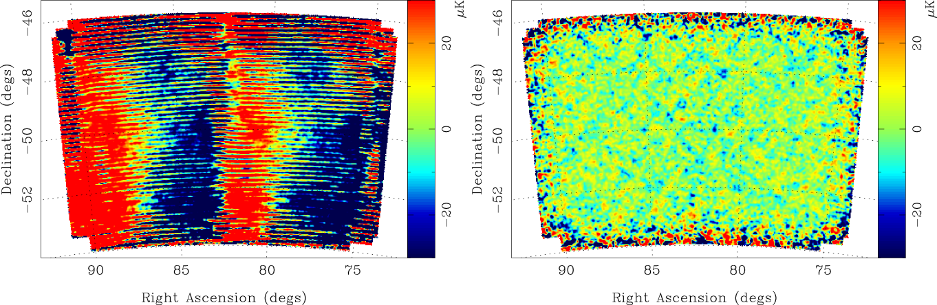
Figure 1.— Demonstration of the performance of the ground templating procedure described in the text. The figure shows maps of the Stokes $U$ polarization over the full QUaD sky area at 150 GHz, smoothed with a 5 arcmin Gaussian kernel. The map on the left is that obtained without removing ground templates and is heavily contaminated by ground pickup. Note the similarity of the contamination between the lead and trail halves of the map. The map on the right is that obtained when we include our templating procedure. Clearly the vast majority of the ground signal is successfully removed by this process. For the purposes of this illustration, in order to highlight the success of the template removal, in both cases, only the mean of each scan was removed from the TOD before mapping. However, for our cosmological analysis, we use maps which have had third-order polynomials removed from each scan (see Figure 2).

Although they will be unbiased estimates of the ground signal, the templates constructed using equation (5) will also contain CMB signal and noise. The expectation value of the constructed templates is

$$\langle\hat{g}(\alpha)\rangle=g(\alpha)+\frac{1}{N_{\rm hits}}\left[\sum_{i\in\Delta\alpha}S_{i}(\theta)+\sum_{i\in\Delta\alpha}n_{i}\right]\,,$$ (6)

where $S_{i}(\theta),g(\alpha)$ and $n_{i}$ are the quantities defined in equation (1). In the limit of a highly redundant scan strategy and uncorrelated noise, the terms in brackets will average to zero and the templates will contain only ground signal. For a realistic scan strategy and correlated noise, these terms will be non-zero and so removing the templates will have the effect of filtering both large-scale CMB signal and long-timescale noise. We correct for this filtering by including the template removal procedure in our Monte-Carlo simulations (Section 6.2).

Finally, to obtain estimates of the TOD which are free of ground pickup, the templates are subtracted from the original TOD:

$$\mathbf{d}^{\rm clean}=\mathbf{d}-\mathbf{A}^{G}\hat{\mathbf{g}}\,,$$ (7)

where $\mathbf{A}^{G}$ is the pointing matrix associated with the ground signal and $\hat{\mathbf{g}}$ is the estimated ground signal constructed using equation (5). This will result in TOD which is, in principle, free of ground contamination and can thus be modeled as in equation (1) but now without the $g(\alpha)$ term. Once the ground contamination has been removed, our map-making proceeds as described in Paper II. Explicitly, we perform the following operations. For each azimuth scan the best-fit third order polynomial is subtracted to remove the long timescale part of the atmospheric $1/f$ noise. For each PSB pair, the data is then summed and differenced to yield temperature ($s_{i}$) and polarization ($d_{i}$) TOD. Maps of the temperature (or Stokes $I$) CMB field are then constructed from the summed data using a simple weighted average:

$$T=\frac{1}{\sum_{i}w_{i}}\sum_{i}w_{i}s_{i}\,,$$ (8)

where the weights are given by $w_{i}=W(x)/v_{\rm scan}$. Here, $v_{\rm scan}$ is the variance of the data across the parent half-scan — noisy data (e.g. ​due to bad weather) is thus down-weighted. $W(x)$, where $x$ denotes the fractional position within the scan, is an apodization (the same for each scan) which we use to down-weight the scan ends. We apply this apodization to reduce the tiling effects seen in our previous analysis (see Section 6.3 and Figure 15 in Paper II) whereby the interaction of the polynomial filtering with different sky coverage for different detectors produced visible step features in the final maps. The exact form used for the apodization is not important.

We construct maps of the Stokes polarization parameters, $Q$ and $U$ as

$$\left(\begin{array}[]{c}Q\\ U\end{array}\right) = \left(\begin{array}[]{cc}\langle\cos^{2}(2\phi_{i})\rangle&\langle\cos(2\phi_{i})\sin(2\phi_{i})\rangle\\ \langle\cos(2\phi_{i})\sin(2\phi_{i})\rangle&\langle\sin^{2}(2\phi_{i})\rangle\\ \end{array}\right)^{-1}$$ (16)

$$\mbox{}\times\left(\begin{array}[]{c}\langle\cos(2\phi_{i})d_{i}\rangle\\ \langle\sin(2\phi_{i})d_{i}\rangle\\ \end{array}\right)\,,$$

where the angled brackets denote an average taken over all data falling within each map pixel and the angle, $\phi_{i}$ is a combination of the polarization sensitivity direction of each detector on the focal plane and the ”deck angle” (rotation about the telescope boresight) of the observation. Note that to construct the averages (e.g. $\langle\cos(2\phi_{i})d_{i}\rangle$) on the right-hand side of equation (16), we also use inverse-variance weights as in equation (8).

Note that the only difference between the approaches of our two pipelines in applying the above operations is during the final coaddition of the template-subtracted data into CMB maps: Pipeline 1 uses HEALPix to pixelize the sky at a resolution of $\sim\!1.7$ arcmin ($N_{\rm side}=2048$). Pipeline 2 works under the flat sky approximation and pixelizes the sky into a 2D cartesian grid with a spacing of $1.2$ arcmin. Figure 1 shows an example of the performance of the template removal procedure (for Pipeline 1) for the $150$ GHz Stokes $U$ polarization map. Note that, in order to highlight the success of the template removal, for this demonstration we have not applied the third order polynomial removal mentioned above to the TOD and have only removed the mean from each scan.

In Figure 2, we present the full set of maps ($T,Q$ and $U$ at $100$ and $150$ GHz; again for Pipeline 1) over the full sky area as estimated using the template removal procedure (now including the third order polynomial removal). For the purposes of visual illustration only, we have smoothed each of the maps with a 5 arcmin Gaussian kernel in order to bring out the CMB structure.

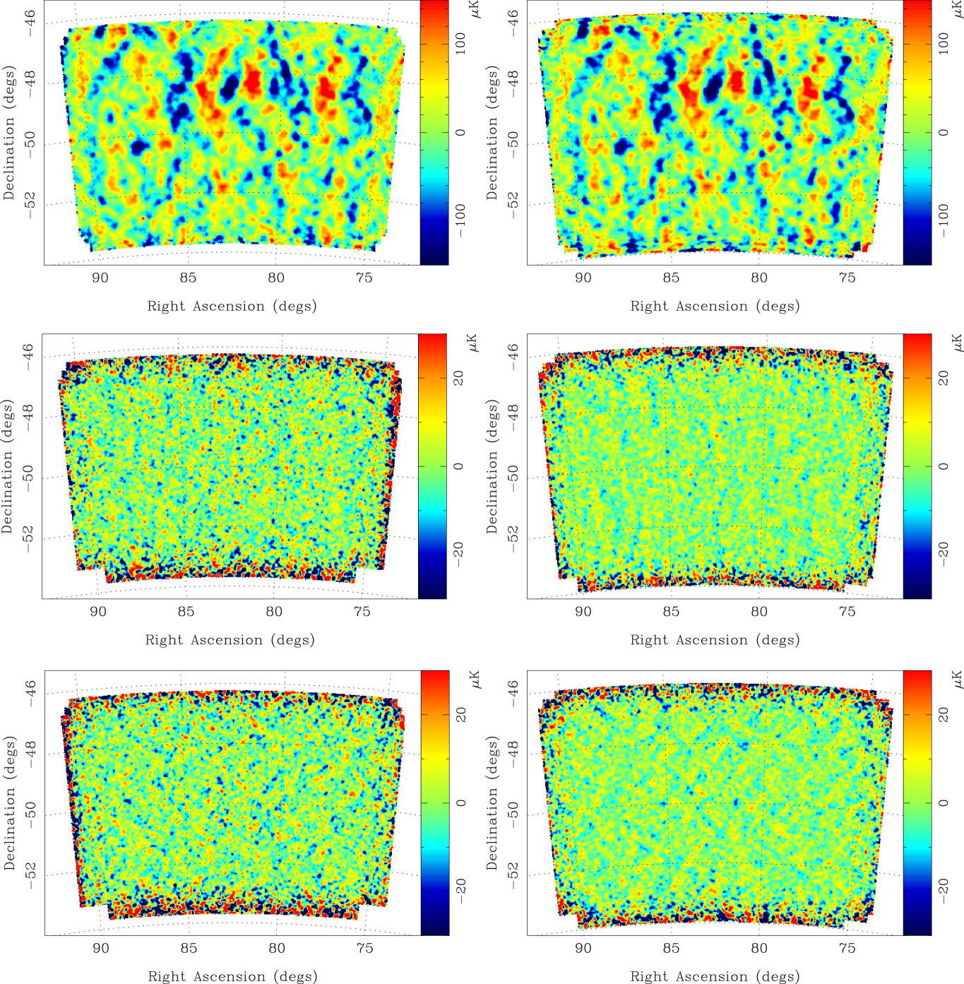
Figure 2.— Maps of the $T$ (top panels), $Q$ (middle panels) and $U$ (lower panels) Stokes parameters over the full QUaD sky area at 100 GHz (left) and 150 GHz (right). For display purposes only, the maps have been smoothed with a 5 arcmin Gaussian kernel. Note the difference in the color stretch used to display the temperature and polarization maps.

We can quickly (and crudely) assess the relative amounts of $E$- and $B$-mode power in the polarization maps by decomposing the $Q$ and $U$ maps into $E$ and $B$ modes. We do this under the flat-sky approximation. To minimize the impact of the noisy edge regions of the maps, and to reduce the effects of $E/B$ mixing due to the finite survey geometry, we apply an apodization to our maps before Fourier transforming. ($E/B$ mixing is fully accounted for during our power spectrum estimation described in Section 6.) The resulting $E$ and $B$ maps at $150$ GHz, are shown in Figure 3. We clearly detect significantly more $E$-mode than $B$-mode structure. The reconstructed $B$-mode map shows similar levels of fluctuations to our polarization jackknife maps (see Section 6.5) and is consistent with noise.

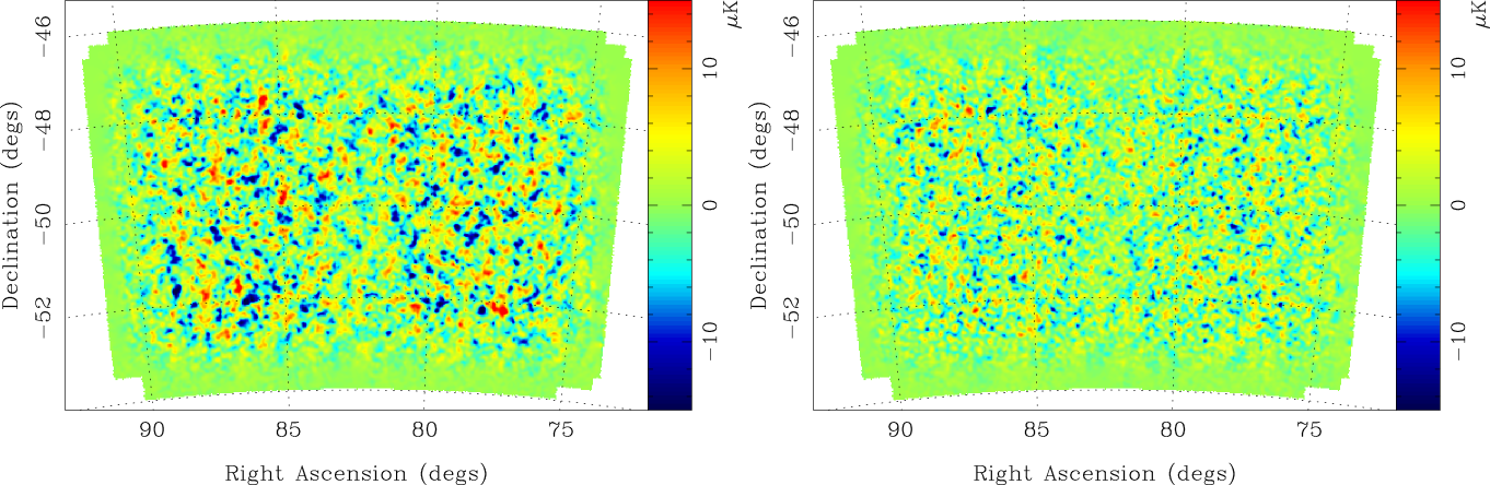
Figure 3.— Apodized 150 GHz QUaD polarization maps decomposed into $E$-modes (left) and $B$-modes (right). Once again, the maps have been smoothed with a 5 arcmin Gaussian kernel. The data is clearly dominated by $E$-modes. The amplitude of fluctuations present in the $B$-mode map is consistent with noise. The slight reduction in the amplitude of fluctuations towards the central RA of the field is due to the application of the apodization mask which down-weights the “seam” between the lead and trail halves of the map.

4. Beam measurements and modeling

Our main set of observations for investigating the QUaD beam shapes are a series of single day observations of the QSO PKS0537-441. In Paper II, our beam model consisted of elliptical Gaussian fits to these QSO observations for each channel.

Given our increased sensitivity, we now include an additional sidelobe component in our beam model. In order to measure the sidelobes from the QSO data, we apply a 6th-order polynomial filter to the TOD before mapping (with the QSO masked) and coadd these data over all channels and over three days of observations. The radially averaged beam profiles measured from these maps reveal the presence of sidelobe structure at just below the -20 dB level, as predicted by the physical optics (PO) simulations of QUaD presented in O’Sullivan et al. (2008). Our two analysis pipelines model these observations in slightly different ways though both are matched to the QSO data.

Pipeline 1 rescales the PO models. The beam profiles which directly result from the PO simulations are not a perfect match to the QSO observations. In particular, the predicted main lobe widths are smaller than observed while the predicted levels of sidelobes are somewhat larger than observed. To match the PO models to the QSO data, we parametrize the models using two parameters, one which scales the main lobe width and one which varies the amplitude of the sidelobes. We then use the observed QSO radial profiles to fit for these parameters. The resulting best-fit re-scaled PO models are used to model the beam.

Pipeline 2 models the beams in a fully empirical manner and is an extension of the model used in Paper II. Using the existing elliptical Gaussian fits to the quasar data, a pure Gaussian simulated beam coadded across channels and observation dates is generated and subtracted from the measured QSO maps. The residual after subtraction is the sidelobe component of the beams. This residual is too noisy to be used directly and so it is radially averaged to produce an (assumed) azimuthally symmetric sidelobe template. This sidelobe template is then added to the original Gaussian elliptical models to produce a fully empirical beam model.

Figure 4 shows the radially averaged profiles measured from the QSO data along with the profiles as predicted using our old elliptical Gaussian beam model and as predicted using our current beam models. Our revised beam models are clearly a superior description of the true beams and are in good agreement — in terms of the resulting beam transfer functions, the two beam models agree to within $4\%$ at 100 GHz and to within $2\%$ at 150 GHz for $\ell<2000$. A description of how we account for the remaining uncertainties on our beams is given in Appendix A.

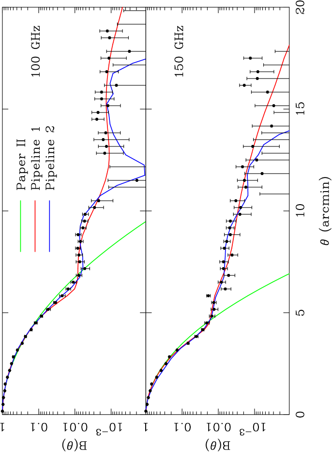
Figure 4.— QUaD beam profiles at 100 GHz (top panel) and 150 GHz (bottom panel) as measured from the QSO PKS0537-441. The radial profiles as predicted using our new beam models for both pipelines are over-plotted as the red and blue curves and show good agreement with the QSO data. Also shown for comparison is the elliptical Gaussian beam model used for our previous analysis in Paper II.

5. Absolute calibration

We derive the absolute calibration of QUaD by cross-correlating our temperature maps with maps from B03 (Masi et al., 2006). This analysis is done in spherical harmonic ($a_{\ell m}$) space following the calibration technique used by Boomerang which, in turn, was calibrated against the WMAP 1st-year maps (Bennett et al., 2003). We apply a correction to the B03 maps to account for the change in calibration (1.25% in temperature) between the 1- and 5-year WMAP analyses (Hinshaw et al., 2009). The B03 maps (which are essentially unfiltered) are first passed through the QUaD simulation pipelines to ensure that they are filtered in an identical manner to the QUaD maps. Taking the spherical harmonic transforms of the maps, the absolute calibration factors for QUaD are then given by

$$S_{\ell}^{\mathrm{quad}}=\frac{B_{\ell}^{\mathrm{\,quad}}\langle a_{\ell m}^{\mathrm{\,b03-X}}a_{\ell m}^{\ast\,\,\mathrm{b03-Y}}\rangle}{B_{\ell}^{\mathrm{\,b03}}\langle a_{\ell m}^{\mathrm{\,b03-X}}a_{\ell m}^{\ast\,\,\mathrm{quad}}\rangle}\,,$$ (17)

where the superscripts, $\!\mathrm{X}$ and $\!\mathrm{Y}$ denote two noise-independent 145 GHz B03 maps and $B_{\ell}^{\mathrm{\,quad}}$ and $B_{\ell}^{\mathrm{\,b03}}$ are the beam transfer functions of the two experiments. This process produces an absolute calibration factor (in $\mu$K/V) as a function of multipole, $\ell$. We take our final absolute calibration factors to be the mean of this value in the range $200<\ell<800$, corresponding to the overlapping scale range of the two experiments. The largest contributors to our calibration error are the quoted B03 uncertainty of $2\%$ and a relative pointing uncertainty between QUaD and B03. Our final calibration uncertainty is 3.4%. Further details on how we estimate this uncertainty are given in Appendix B.

6. Power spectrum analysis

To estimate the CMB power spectra, as in Paper II, we adopt a Monte-Carlo (MC) based technique whereby we rely on accurate simulations of the experiment to correct for the effects of noise, beams, timestream filtering and the removal of the ground templates. Before describing the MC simulations, we first describe the differences between our two pipelines in their approach to power spectrum estimation.

6.1. Power spectrum estimation

Both of our pipelines broadly follow the so-called pseudo-$C_{\ell}$ technique (Hivon et al., 2002), extended to polarization (Brown et al., 2005). Note that, for both pipelines, in order to minimize edge effects, the $T,Q$ and $U$ maps are first apodized with an inverse-variance mask as described in Section 6.1 of Paper II.

Pipeline 1 works on the curved sky and uses fast spherical harmonic transforms to estimate the pseudo-$C_{\ell}$ spectra. These spectra are then corrected for the effects of the sky cut, noise and filtering, and binned into band powers according to

$${\bf P}_{b}=\sum_{b^{\prime}}{\bf K}^{-1}_{bb^{\prime}}\,\sum_{\ell}P_{b^{\prime}\ell}\,(\widetilde{\bf C}_{\ell}-\langle\widetilde{\bf N}_{\ell}\rangle_{MC})\,.$$ (18)

In this equation and throughout this section, we use bold-face to denote six-spectrum quantities, e.g.​ ${\bf P}_{b}$ is a $6\,n_{\,\rm band}$ vector, ${\bf P}_{b}=\{P_{b}^{TT},P_{b}^{EE},P_{b}^{BB},P_{b}^{TE},P_{b}^{TB},P_{b}^{EB}\}$, and ${\bf K}_{bb^{\prime}}$ is a $6\,n_{\,\rm band}\times 6\,n_{\,\rm band}$ matrix, given by

$${\bf K}_{bb^{\prime}}=\sum_{\ell}P_{b\ell}\sum_{\ell^{\prime}}{\bf M}_{{\ell\ell^{\prime}}}F_{\ell^{\prime}}Q_{{\ell^{\prime}}b^{\prime}}\,.$$ (19)

In equation (18), $\widetilde{\bf C}_{\ell}$ are the pseudo-$C_{\ell}$ spectra estimated from the data maps and $\langle\widetilde{\bf N}_{\ell}\rangle_{MC}$ are the noise power spectra as measured from simulations.

$P_{b\ell}$ is a binning operator which bins the raw pseudo-$C_{\ell}$ into band powers and $Q_{\ell b}$ is the inverse operator which “unfolds” a band power into individual $C_{\ell}$s. For this analysis, we use “flat” band powers for which the quantity, $\ell(\ell+1)C_{\ell}/2\pi$ is constant within each band. That is, the binning operator we use is

$$P_{b\ell}=\left\{\begin{array}[]{ll}\frac{1}{2\pi}\frac{\ell(\ell+1)}{\ell^{(b+1)}_{\rm low}-\ell^{(b)}_{\rm low}},&\mbox{ if }2\leq\ell^{(b)}_{\rm low}\leq\ell<\ell^{(b+1)}_{\rm low}\\ 0,&\mbox{ otherwise, }\end{array}\right.$$ (20)

with the corresponding inverse operator given by

$$Q_{\ell b}=\left\{\begin{array}[]{ll}\frac{2\pi}{\ell(\ell+1)},&\mbox{ if }2\leq\ell^{(b)}_{\rm low}\leq\ell<\ell^{(b+1)}_{\rm low}\\ 0,&\mbox{ otherwise, }\end{array}\right.$$ (21)

where $\ell^{(b)}_{\rm low}$ denotes the nominal lower edge of band $b$.

The coupling matrix, ${\bf M}_{{\ell\ell^{\prime}}}$, describes the mode-mixing effects of the apodization mask and sky cut and is given in Brown et al. (2005) for the full set of six possible CMB spectra. Note that the ${\bf M}_{{\ell\ell^{\prime}}}$ matrix fully encodes $E/B$ leakage effects due to the finite survey geometry and so our Pipeline 1 estimator explicitly corrects the $EE$ and $BB$ spectra for this leakage in the mean.

$F_{\ell}$ is a transfer function which we use to describe the combined effects of timestream filtering, beam suppression and filtering of the sky signal due to the removal of the ground templates. This function will also encode any other signal suppression effects which are present in our simulations (e.g. pixelization effects). We estimate $F_{\ell}$ from our signal-only simulations as described in Section 6.3.

Pipeline 2 works in the flat sky approximation and uses 2D FFTs to estimate power spectra. This pipeline is described in detail in Paper II. The power spectrum estimator for Pipeline 2 can effectively be written as

$${\bf P}_{b}=\,F_{b}^{-1}\sum_{\ell}P_{b\ell}\,(\widetilde{\bf C}_{\ell}-\langle\widetilde{\bf N}_{\ell}\rangle_{MC})\,,$$ (22)

where $F_{b}$ is the binned equivalent of the per-multipole transfer function, $F_{\ell}$ and we have implicitly made the connection between the flat sky and curved sky power spectra, $C_{\ell}\approx P(k)$ for $\ell\approx 2\pi k$.

Note that (in addition to the flat sky approximation), the primary difference between the two pipelines is that Pipeline 1 performs the correction for the mode-mixing effects induced by the sky cut whereas Pipeline 2 does not perform this correction. Because of this difference, neither the recovered band powers nor their uncertainties are directly comparable between the two pipelines. A proper comparison of the two analyses requires the use of the associated band power window functions (Section 6.3) which fully encode the relation between underlying true sky power and observed power for both pipelines.

In both analyses, we estimate the covariance matrix of our power spectrum estimates from the scatter found in the power spectra measured from simulations containing both signal and noise:

$$\langle\Delta{\bf P}_{b}\Delta{\bf P}_{b^{\prime}}\rangle=\langle({\bf P}_{b}-\overline{\bf P}_{b})({\bf P}_{b^{\prime}}-\overline{\bf P}_{b^{\prime}})\rangle_{MC}\,,$$ (23)

where $\overline{\bf P}_{b}$ denotes the average of each band power over all simulations. Note finally that the covariance properties of the power spectra estimates are dependent on whether the correction for mode-mixing induced by the sky cut is applied or not. We return to this issue in Section 6.6 where we compare the results from our two analyses.

6.2. Simulations

In simulating QUaD, we follow the procedure described in Section 5 of Paper II with some important differences, which we now discuss. Algorithmically both of our analysis pipelines adopt the same approach to creating simulated timestreams and only differ in the final map-making stage as described in Section 3.2.

6.2.1 Signal simulations

To create the signal component in the simulations, we first generate model $TT,EE,TE$ and $BB$ CMB power spectra using CAMB (Lewis et al., 2000). The input cosmology consists of the best-fitting $\Lambda$CDM model to the 5-year WMAP data set (Dunkley et al., 2009). Note that the model spectra used include the effects of CMB lensing and so the input $B$-mode power is non-zero. (For comparison, in Paper II, our input model was the best-fit to the 3-year WMAP data set and our input $B$-mode power was set to zero.)

Realizations of CMB skies are then generated from these model spectra using a modified version of the HEALPix software. These maps are generated at a resolution of 0.4 arcmin ($N_{\rm side}=8192$). The simulated maps are then projected onto a 2D cartesian grid and convolved with the beam model for each detector channel. The resolution used for this intermediate map is 0.6 arcmin. The generation of the sky maps for each detector and deck angle and interpolation to simulated TOD then proceeds exactly as described in Section 5.1 of Paper II.

6.2.2 Noise simulations

In order to simulate realistic noise, we must first measure the noise properties from the real data. However, the undifferenced data contains not only noise but also CMB signal and ground signal (see equation 1). The instantaneous signal-to-noise in the timestream is negligible and so the CMB component can be safely ignored. However, the same is not true for the ground signal which, in some cases, is a very significant component in the timestream, particularly in polarization. The data must therefore be cleaned of the ground component before measuring the noise power spectra.

One might think that the best way to achieve this would be to measure the noise spectra from data which has been template subtracted using equation (7). Such a procedure could, in principle, be iterated and is similar to procedures suggested for measuring the noise properties of CMB data when the signal component is non-negligible (e.g. ​Ferreira & Jaffe 2000). However, as noted in Section 3.2, our template removal procedure filters the noise in a non-trivial fashion. In particular, because of the non-uniform azimuth coverage of the scan strategy, the ground templates are noisier at each end than they are in the central regions. The result is that after subtracting the templates, the noise is no longer uniform and this prohibits its characterization through simple FFT-based power spectrum estimators — since the noise is no longer a stationary Gaussian random process, a power spectrum description will fail.

To avoid these complications, we have measured the noise properties of the TOD from data which has been lead-trail differenced. The differencing efficiently removes the ground signal while under the assumption that the noise is stationary over a $30$ minute timescale, the power spectra of the undifferenced TOD are simply the spectra measured from the differenced TOD divided by 2. For each pair of lead-trail observations, we therefore assign the power spectra measured from the differenced data, appropriately normalized, to each of the lead and trail scan-sets. Simulated noise-only timestreams are then generated exactly as described in Section 5.2 of Paper II.

Examining the QUaD data and comparing it to simulated data obtained using the above process, there are occasions where our assumption of stationarity over a $30$ minute timescale is not satisfied. However, for the majority of the data the assumption is good and it is only ever a poor one for our temperature analysis. Moreover, a thorough comparison of the statistics of the simulated and real data indicates that our procedure provides an excellent description of the noise properties of the undifferenced data when averaged over each day for both temperature and polarization. Further averaging over tens of pixels and hundreds of observation dates will result in these rare failures of our noise model having a negligible impact on the results.

Once generated, both the signal-only and noise-only simulated TOD are processed into $T,Q$ and $U$ maps in an identical manner to that used for the real data. In particular, note that both the ground template subtraction and polynomial filtering are applied also to the simulated data and so the effects of filtering on both the signal and on the noise are fully accounted. Finally, to obtain simulated maps containing both signal and noise, we simply add the signal-only and noise-only maps. Since all of our data processing steps are linear operations, this final step results in simulated maps no different to those which would have been obtained if we had instead summed the signal-only and noise-only TODs, and is computationally more efficient.

6.3. Transfer functions and band power window functions

We estimate the transfer function from our suite of signal-only simulations. In the absence of noise, the mean of the recovered pseudo-$C_{\ell}$ spectra will equal their expectation values,

$$\langle\widetilde{\bf C}_{\ell}\rangle_{MC}=\sum_{\ell^{\prime}}{\bf M}_{\ell\ell^{\prime}}F_{\ell^{\prime}}{\bf C}_{\ell^{\prime}}\,,$$ (24)

where ${\bf C}_{\ell}$ are the input model spectra used to create the simulations. For a small-area survey such as QUaD, the unbinned coupling matrix, ${\bf M}_{\ell\ell^{\prime}}$, is singular and so equation (24) cannot be solved directly. In Pipeline 1, we iteratively solve this equation to provide an estimate of $F_{\ell}$. With a reasonable starting guess, convergence is typically reached in just a few iterations. For Pipeline 1, the band power window functions, ${\bf W}_{b\ell}$, defined by (Knox, 1999),

$$\langle{\bf P}_{b}\rangle=\sum_{\ell}\frac{{\bf W}_{b\ell}}{\ell}\frac{\ell(\ell+1)}{2\pi}\langle{\bf C}_{\ell}\rangle\,,$$ (25)

are given by

$$\frac{{\bf W}_{b\ell}}{\ell}=\frac{2\pi}{\ell(\ell+1)}F_{\ell}\,\sum_{b^{\prime}}{\bf K}^{-1}_{bb^{\prime}}\sum_{\ell^{\prime}}P_{b^{\prime}{\ell^{\prime}}}{\bf M}_{\ell^{\prime}\ell}\,.$$ (26)

Pipeline 2 calculates its band power window functions numerically as described in Section 6.6 of Paper II. In order to calculate the transfer functions, Pipeline 2 simply takes the ratio of the mean band powers recovered from signal-only simulations and the expectation values for each band power:

$$F_{b}=\frac{\sum_{\ell}P_{b\ell}\langle\widetilde{\bf C}_{\ell}\rangle_{MC}}{\langle{\bf P}_{b}\rangle}\,.$$ (27)

Figure 5 shows the derived transfer function from Pipeline 1. (The transfer function from Pipeline 2 is similar.) As mentioned earlier, this function encapsulates all effects due to timestream filtering, beam suppression and the filtering due to removal of the ground templates. To demonstrate the relative size of these effects, we also plot the transfer function derived from special simulations with these three effects included in isolation. Of particular interest is the transfer function describing the ground-removal procedure — this curve, in effect encapsulates the lossiness of the technique. On scales where this curve is $\mathrel{\hbox to0.0pt{\lower 4.0pt\hbox{\hskip 1.0pt$\sim$}\hss}\raise 1.0pt\hbox{$>$}}0.5$, we gain an improvement over the field-differencing technique. We see that below $\ell\sim 200$, there is little gain from our template-removal technique over field-differencing. The amount of signal retained then climbs rapidly and is effectively unity by $\ell=1000$.

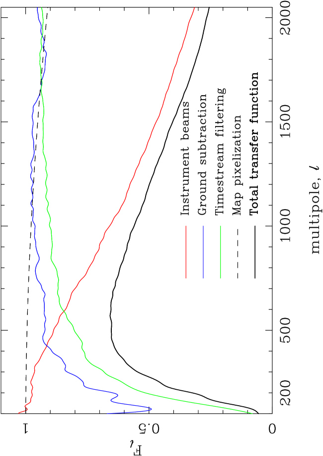
Figure 5.— Total transfer function, $F_{\ell}$ (black curve) as measured in our Pipeline 1 analysis for the 150 GHz channel. Also shown are the transfer functions for timestream filtering (green), ground-template removal (blue) and beam suppression (red) in isolation. The dashed curve shows the suppression of signal due to map pixelization for a HEALPix resolution, $N_{\rm side}=2048$. The total transfer function is the product of these four individual curves.

Figure 6 shows the band power window functions (BPWFs), plotted as $W_{b\ell}/\ell$, for $C^{BB}_{\ell}$ from both our pipelines for the 150 GHz channel. These functions describe the response of our band power measurements to the true sky signal at each multipole. The negative wings in the BPWFs of Pipeline 1 are a direct result of the application of the correction for mode-mixing effects as described in Section 6.1.

The expectation values for our $EE$ band powers assuming the best-fit $\Lambda$CDM model to the WMAP 5-year data are shown in Figure 7. Note that the apparent improvement in going from Pipeline 2 to Pipeline 1 in terms of the agreement between the true sky power and the band power expectation values does not come without a price — as a result of applying the mode-mixing correction, the error bars for Pipeline 1 are enhanced with respect to the Pipeline 2 errors. The covariance properties also change between the two analyses such that the total information content is preserved.

We emphasize that, in terms of either the accuracy or the precision of the recovery of true sky power, neither analysis is superior. This is clear from the fact that one can transform between the band power estimates and covariances of the two analyses via a simple and exact matrix operation. Whether to apply the mode-mixing correction is simply a matter of preference and is only relevant for visual interpretation of the results — one can choose to have smaller error bars or one can choose to have band powers which better trace the underlying true sky power but one cannot have both.

Figure 6.— Band power window functions for Pipeline 1 (top panels) and Pipeline 2 (bottom panels) for the $C^{BB}_{\ell}$ power spectrum. The blue curves show the response to true $BB$ power and the red lines show the response to $EE$ power.

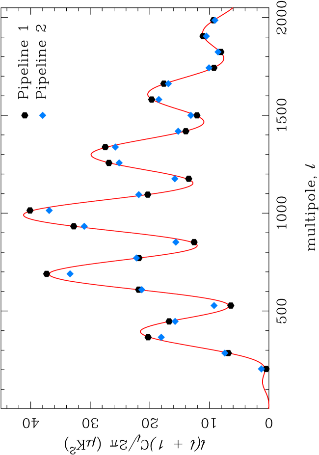
Figure 7.— Expectation values for the $\Lambda$CDM $E$-mode power spectrum for both pipelines at 150 GHz. The mapping of true sky power to observed band powers for both pipelines is fully encoded in their associated band power window functions (Figure 6).

6.4. Power spectrum results

We apply the procedures described in Section 6.1 to estimate the six possible CMB power spectra ($TT,TE,EE,BB,TB,EB$) from the QUaD maps. In addition to the 100 and 150 GHz auto-spectra, we also estimate the 100-150 GHz cross-spectra as described in Paper II. In the case where the noise is uncorrelated between the two frequency channels, the cross spectra do not require the noise-debiasing step. Although, in practice, we do apply this correction, the correction is modest for the cross spectra so these measurements will be much less sensitive to the details of our noise model. The power spectrum results from Pipeline 1 are presented in Figure 8. We make strong detections of the $TT$, $TE$ and $EE$ spectra which show good agreement with those predicted by the best-fitting $\Lambda$CDM model to the 5-year WMAP results. The $BB$, $TB$ and $EB$ spectra are consistent with null within the noise. The results from Pipeline 2 show a similar agreement with the $\Lambda$CDM model.

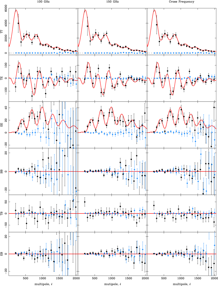
Figure 8.— Full set of power spectrum results from Pipeline 1 where the quantity plotted in the y-direction is $\ell(\ell+1)C_{\ell}/2\pi$. The red curves are the spectra predicted by the best-fit $\Lambda$CDM model to the WMAP 5-year data (Dunkley et al., 2009). The blue points show the power spectra measured from our deck angle differenced maps and represent a stringent test for residual ground contamination — see the text of Section 6.5 for details.

6.5. Jackknife tests

We have subjected our analysis to the same set of systematic tests as performed in Paper II. These tests involve splitting the data into two roughly equal parts. Maps made from the two data subsets are subtracted and the power spectra of the residual maps are calculated. Any deviation of these “jackknife” spectra from null would indicate systematic contamination in the data. For a detailed description of the various ways in which we split the data, we refer the reader to Section 7 of Paper II.

The strongest test is the so-called “deck jackknife” test where we split the data according to the boresight rotation angle (deck angle) of the observations. This test, in particular, will be strongly sensitive to any residual ground contamination remaining in the data after applying the procedure described in Section 3. In Figure 8, the deck jackknife spectra are plotted alongside the spectra measured from the undifferenced maps. It is clear from this figure that the power measured in the deck-differenced maps is small compared to the measured signals in $TT$, $TE$ and/or $EE$. The other data splits which we consider are splitting the data according to orientation of the PSB pairs on the focal plane (see Section 2), a split between the forward and backward scans and a split in observation dates which roughly separates the data into the 2006 and 2007 observing seasons. We also take the difference of the 100 and 150 GHz maps. This “frequency jackknife” test is not strictly a test for systematic effects in the data. Rather, it is a strong test for “foreground” (i.e. ​non-CMB) astrophysical emission.

The cancellation of the signal apparent in Figure 8 is visually impressive. To investigate whether the differenced spectra are formally consistent with null, as in Paper II, we have performed $\chi^{2}$ tests against the null model. Note that we compare this statistic with the $\chi^{2}$ distribution as measured from our simulations rather than against the theoretical $\chi^{2}$ curve, calculating the “probability to exceed” (PTE) the observed value by random chance. Low numbers therefore indicate a problem. The PTE values for each of our measured spectra (from Pipeline 1) are presented in Table 6.5.

Table 1Jackknife PTE values from $\chi^{2}$ tests

Jackknife	$TT$	$TE$	$EE$	$BB$	$TB$	$EB$
Deck angle:
100 GHz	0.000	0.415	0.883	0.933	0.598	0.917
150 GHz	0.008	0.295	0.963	0.988	0.258	0.423
Cross	0.000	0.028	0.780	0.197	0.287	0.527
Scan direction:
100 GHz	0.008	0.017	0.122	0.812	0.478	0.518
150 GHz	0.080	0.665	0.755	0.153	0.515	0.485
Cross	0.000	0.608	0.155	0.783	0.487	0.263
Split season:
100 GHz	0.743	0.287	0.350	0.655	0.840	0.413
150 GHz	0.000	0.387	0.242	0.022	0.340	0.647
Cross	0.273	0.065	0.110	0.160	0.630	0.850
Focal plane:
100 GHz	0.173	0.872	0.690	0.813	0.703	0.672
150 GHz	0.530	0.397	0.910	0.988	0.933	0.715
Cross	0.270	0.012	0.493	0.105	0.735	0.578
Frequency	0.000	0.362	0.418	0.588	0.208	0.783
difference

Examining the table, the PTE values for all the spectra bar $TT$ reveal no significant problems, the numbers being consistent with a uniform distribution between zero and one. In contrast, many of our $TT$ jackknife spectra are clearly inconsistent with a null signal. The failure is perhaps excusable in the case of the frequency difference (since there are astrophysical reasons why this test might fail) but taken as a whole, the statistics for $TT$ (and to a lesser extent, some of the $TE$ numbers) suggest that there is some degree of residual systematics present in our temperature maps. The PTE statistics for Pipeline 2, although not identical, show the same general pattern of jackknife failures for the $TT$ spectra. Comparing to our previous results, there were hints of a problem with the $TT$ jackknife tests in Paper II but to a lesser extent than is apparent now. This is possibly due to the fact that with our increased sensitivity we can measure both the signal and systematics to greater precision. Alternatively, it could indicate that the template removal procedure is not as effective as field-differencing in removing the ground.

These jackknife failures indicate that residual systematic effects in our temperature maps are significant with respect to the errors on the jackknife spectra. However, the jackknife errors contain only noise whereas the errors on our measured $TT$ and $TE$ CMB power spectra also contain considerable sample variance. To assess how significant the residual systematics are, in Figure 9, we plot the measured $TT$ and $TE$ jackknife band powers alongside the signal band powers for the 150 GHz channel. Clearly, when compared to the sample variance dominated signal spectra, the degree of residuals are much less significant. Repeating the $\chi^{2}$ analysis using the signal covariance matrices in place of the jackknife covariance matrices, we find that the residual contamination is negligible. In summary, although our TT jackknife tests indicate the presence of residual systematics, they also clearly demonstrate that these residuals are irrelevant compared to both the measured sky signal and its associated sample variance. Note this is also true for the levels of foreground contamination in our maps since our frequency difference test is sensitive to foregrounds.

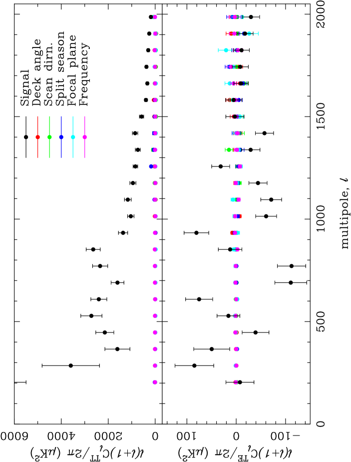
Figure 9.— Signal and jackknife $TT$ (top panel) and $TE$ (bottom panel) power spectra for the 150 GHz channel. The black points show the measured signal spectra and the colored points are the jackknife spectra. The levels of power measured in the jackknife maps are negligible when compared to the sample variance driven errors on the signal spectra.

6.6. Examination of final power spectra

To produce a set of final power spectra, we combine the single-frequency and 100-150 GHz cross spectra shown in Figure 8 following the procedure described in Section 9 of Paper II. The final estimates of the power spectra are shown in Figure 10 for both of our analysis pipelines. Once again, the model curves plotted are the best-fitting $\Lambda$CDM model to the WMAP 5-year results. We have performed $\chi^{2}$ tests of all spectra and both analyses show perfectly acceptable agreement with this model and with each other. Pipeline 1 $\chi^{2}$ and PTE values are given in Table 6.6.

Table 2$\chi^{2}$ tests of the combined spectra against the $\Lambda$CDM and null models.

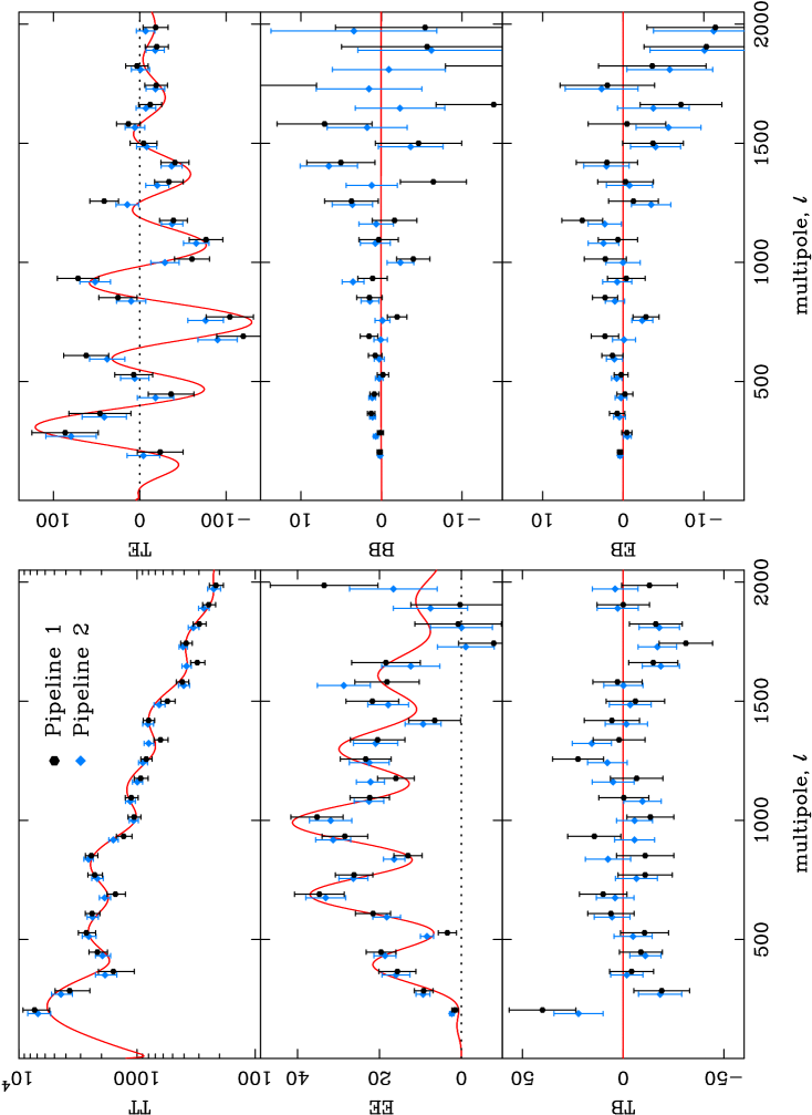
Figure 10.— Final power spectrum results obtained from an optimal combination of the 100 GHz, 150 GHz and cross-frequency power spectra. Spectra from both pipelines (again, plotted as $\ell(\ell+1)C_{\ell}/2\pi$) are shown in comparison to the expected spectra in the concordance $\Lambda$CDM model. Note the $TT$ power spectrum is plotted with a log-scale in the y-axis. For clarity, the two sets of points have been slightly offset in the horizontal direction.

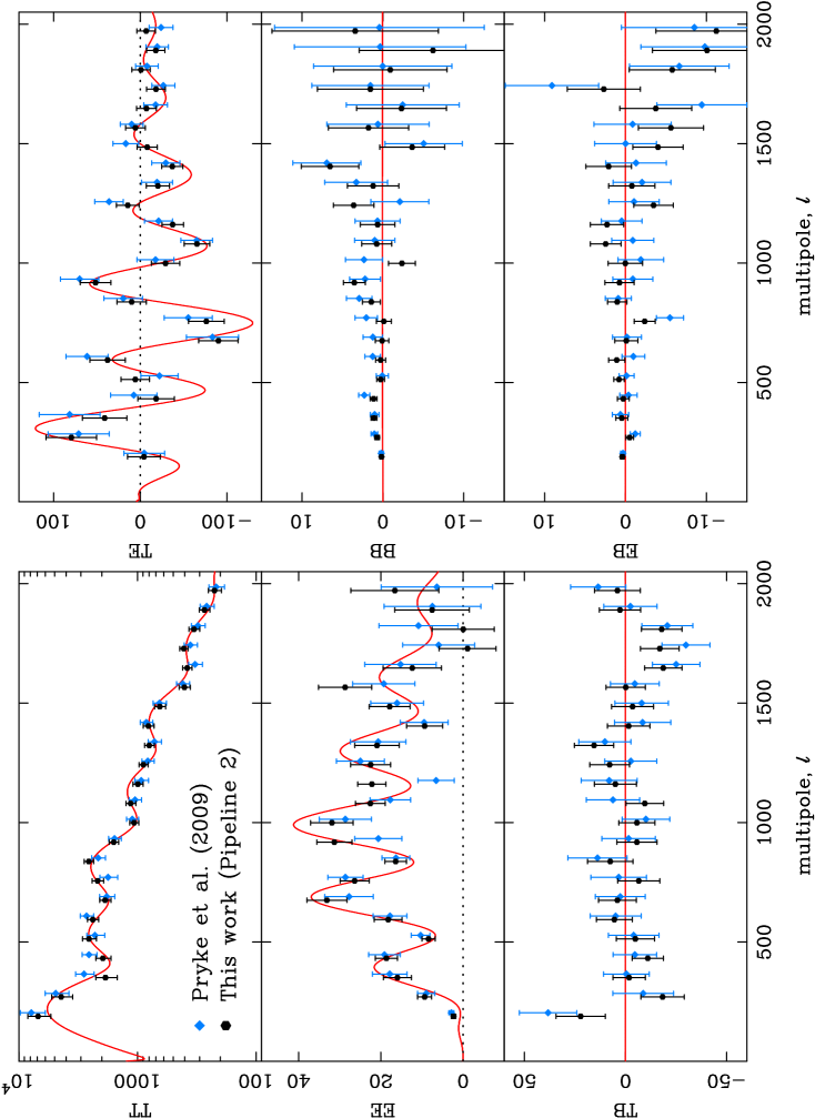
Figure 11.— Comparison of our final power spectra from Pipeline 2 with the field-differenced analysis of Pryke et al. (2009). The uncertainties on our band power measurements have been reduced by $\sim 30\%$ and our new beam models result in a small increase in amplitude in the measured spectra for multipoles, $\ell\mathrel{\hbox to0.0pt{\lower 4.0pt\hbox{\hskip 1.0pt$\sim$}\hss}\raise 1.0pt\hbox{$>$}}700$. For clarity, the two sets of points have been slightly offset in the horizontal direction.

Comparing the two sets of results presented in Figure 10 we see that the nominal error-bars are smaller for Pipeline 2 and that the Pipeline 2 points appear to trace a slightly smoothed version of the Pipeline 1 points. Both of these effects are simply a result of the differing band power window functions as discussed in Section 6.3. Note that neighboring band powers in Pipeline 1 are $\sim 10\%$ anti-correlated whereas they are $\sim 10\%$ positively correlated in Pipeline 2. Correlations between non-adjacent band powers are negligible for both analyses.

Figure 11 shows a comparison with our previous results from Paper II. Note that we perform this comparison using Pipeline 2 since this pipeline is an extension of the analysis presented in Paper II and so is directly comparable. Two effects are apparent in this figure. First, the uncertainties on all of our power spectra have been reduced by $\sim 30\%$ as a result of the increase in sky area afforded by our template-based ground removal technique. Second, implementing the improved beam models described in Section 4 has resulted in a slight increase in the amplitude of our power spectrum measurements for multipoles, $\ell\mathrel{\hbox to0.0pt{\lower 4.0pt\hbox{\hskip 1.0pt$\sim$}\hss}\raise 1.0pt\hbox{$>$}}700$. This impacts mostly on the high signal-to-noise measurements of the $TT$ spectrum on small scales.

Figure 12 shows our measured power spectra from Pipeline 1 in comparison with the published results from a number of other CMB experiments.

The QUaD power spectra data, along with the associated band power covariance matrices and band power window functions (for both of our analysis pipelines) are available for download at http://quad.uchicago.edu/quad.

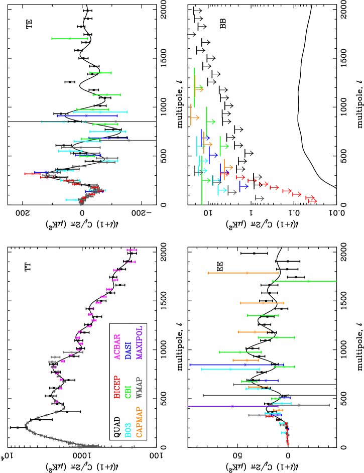
Figure 12.— QUaD measurements of the $TT$, $TE$ $EE$ and $BB$ power spectra compared to results from the WMAP (Nolta et al., 2009), ACBAR (Reichardt et al., 2009), BICEP (Chiang et al., 2009), B03 (Piacentini et al., 2006; Montroy et al., 2006), CBI (Sievers et al., 2007), CAPMAP (Bischoff et al., 2008), MAXIPOL (Wu et al., 2007) and DASI (Leitch et al., 2005) experiments. The $BB$ measurements are plotted as 95% upper limits. The smooth black curves in each panel are the power spectra expected in the best-fit $\Lambda$CDM model to the WMAP 5-year data.

6.7. Acoustic oscillations in the $E$-mode power spectrum

We have assessed the significance with which we detect the acoustic oscillations in the $EE$ power spectrum by repeating the analysis of Section 9.3 in Paper II. For this test, we compare our $EE$ measurements against both the $\Lambda$CDM model and against a heavily smoothed version of the $\Lambda$CDM curve. The results of this test are shown in Figure 13. The QUaD detection of acoustic oscillations in the $E$-mode power spectrum is now beyond question – the probability that the true $E$-mode spectrum is a smooth curve has dropped from $0.001$ with our previous analysis to $<10^{-14}$. We have also repeated our Paper II analysis where we used “toy models” of the $E$-mode spectrum to fit the peak spacing, phase and amplitude of the acoustic oscillations. With our previous measurements, we constrained the peak spacing to be $\Delta\ell_{s}=306\pm 10$, the phase to be $\phi=13^{\circ}\pm 33^{\circ}$ and the amplitude to be $a=0.86\pm 0.17$. Repeating the analysis with our new measurements, we find $\Delta\ell_{s}=308\pm 7$, $\phi=6^{\circ}\pm 22^{\circ}$ and $a=0.96\pm 0.10$. For comparison, when we perform the analysis with the QUaD band power values replaced by their expectation values in the $\Lambda$CDM model, we find $\Delta\ell_{s}=310$, $\phi=13^{\circ}$ and $a=0.99$. These results confirm that the polarization peak spacing and the phase relationship between the temperature and polarization acoustic oscillations are as expected in the $\Lambda$CDM model. Passing this (non-trivial) test further strengthens the foundations of this model.

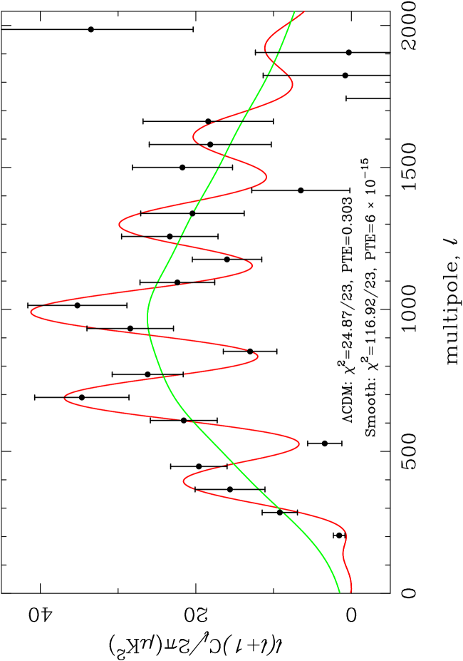
Figure 13.— QUaD’s measurements of the $EE$ spectrum (black points) compared to the $\Lambda$CDM model (red curve) and a model without peaks (green curve). The data are incompatible with the no-peak scenario — the probability that the smooth curve is correct is $<10^{-14}$.

7. Cosmological interpretation

The QUaD results presented in this paper are the most precise determination of the CMB polarization, and of its correlation with the CMB temperature, at angular scales $\ell>200$, to date. Within the standard $\Lambda$CDM model, given a precise measurement of the $TT$ power spectrum (e.g. from WMAP), the $TE$ and $EE$ spectra on all but the very largest scales are deterministically predicted. Nevertheless, sufficiently accurate measurements of these spectra can still tighten constraints on cosmological parameters. In particular, precise measurements of the $TE$ and $EE$ acoustic peaks and valleys can help constrain the cosmological parameters which determine this peak pattern.

Beyond the standard $\Lambda$CDM model, power spectrum measurements from small-scale experiments such as QUaD can add further information. Two such extensions to the $\Lambda$CDM model which are well-motivated in the context of single-field slow-roll inflation models are a possible tensor component in the primordial perturbation fields and a scale dependence (or “running”) in the scalar spectral index. Placing constraints on tensor modes through measurements of the large-scale $B$-mode polarization induced by a gravitational wave background from inflation is a major goal of ongoing and future CMB polarization experiments. Although the scales probed by QUaD’s polarization measurements are too small to constrain this $B$-mode signal directly, QUaD can help through its ability to constrain the scalar spectra index, $n_{s}$, since this parameter is correlated with the tensor-to-scalar ratio. For a $\Lambda$CDM model extended to include a running in $n_{s}$, measurements of the high-$\ell$ temperature power spectrum can be useful in constraining both $n_{s}$ and the degree of running.

In this section, we constrain cosmological models by adding the QUaD temperature and polarization data (i.e. ​our new measurements of the $TT$, $EE$, $TE$ and $BB$ spectra) to the results of two other CMB experiments — the WMAP 5-year analysis (Nolta et al., 2009) and the final results from the ACBAR experiment (Reichardt et al., 2009). We will also investigate the effect of adding large-scale structure data by including measurements of the present-day matter power spectrum, $P(k)$ from the SDSS Luminous Red Galaxy (LRG) 4th data release (Tegmark et al., 2006).

In this paper, we focus on what the QUaD dataset taken as a whole adds to parameter constraints. In addition to investigating further extensions to the $\Lambda$CDM model, we will fully explore the consistency of our temperature-only and polarization-only parameter constraints in a future paper (Gupta et al., in prep). See also Castro et al. (2009) for temperature-only and polarization-only constraints obtained using our previous power spectrum results of Paper II.

7.1. Methodology

To obtain our constraints, we perform a Monte-Carlo Markov Chain (MCMC) sampling of the cosmological parameter space. To do this, we use the publicly available CosmoMC package (Lewis & Bridle, 2002), which in turn uses the CAMB code (Lewis et al., 2000) to generate the CMB and matter power spectra.

We make use of the publicly available WMAP likelihood software from the LAMBDA website. We marginalize over a possible contribution to the temperature power spectrum from the Sunyaev-Zel’dovich (SZ) effect following the WMAP analysis (Dunkley et al., 2009). To do this, we use the SZ templates from Komatsu & Seljak (2002) (also available from the LAMBDA website) and the known frequency dependence of the SZ effect. In order to avoid possible contamination from residual point sources, we exclude the ACBAR band powers above $\ell=2000$. For the same reason, we do not include our own $TT$ measurements at $\ell>2000$ (Friedman et al., 2009).

Marginalization over the WMAP beam uncertainty is included in the WMAP likelihood code and we also marginalize over the quoted ACBAR calibration and beam uncertainties. We take the latter to be a 2% error on a 5 arcmin (FWHM) Gaussian beam as assumed in the ACBAR CosmoMC data file. For QUaD, we marginalize over our 3.5% calibration uncertainty and over the uncertainty in our beam. As described in Appendix A, our beam uncertainties are dominated by uncertainties in the level of our sidelobes rather than in the effective FWHM of our main lobe beams. We therefore marginalize over the full $\ell$-dependent beam uncertainty shown in Figure 19. Where we include the SDSS LRG data, we marginalize over both the amplitude of the matter power spectrum and over a correction for scale-dependent non-linear density evolution using the methods described in Tegmark et al. (2006).

We model the likelihood functions for the QUaD auto-spectra as offset log-normal distributions (Bond et al., 2000). The required noise-offsets are derived from our signal-only and noise-only simulations. (We model the $TE$ likelihood as a Gaussian distribution.) We include all covariances apparent (above the numerical noise) in our simulation-derived covariance matrix (equation 23). In addition to same-spectrum covariances, this includes non-zero $TT$-$TE$, $EE$-$TE$, $TT$-$EE$ and $EE$-$BB$ correlations.

Note that, for our main MCMC analysis, we do not include our measurements of the parity-violating spectra, $TB$ and $EB$ since these spectra are expected to vanish in standard $\Lambda$CDM models and its usual variants. However, in Section 7.7, we will use these spectra to constrain possible parity-violating interactions to the surface of last scattering (see e.g. Lue et al. 1999) following our previous work (Wu et al., 2009).

Finally, in Section 7.8, we use our polarization measurements to place a formal upper limit on the strength of the lensing $B$-mode signal.

Our basic $\Lambda$CDM cosmological model is characterized by the following six parameters (where $h=H_{0}/\left[100\,\,{\rm kms}^{-1}{\rm Mpc}^{-1}\right]$, $H_{0}$ being Hubble’s constant in units, kms^-1Mpc^-1): the physical baryon density, $\Omega_{b}h^{2}$; the physical cold dark matter density, $\Omega_{c}h^{2}$; the ratio of the sound horizon to the angular diameter distance at last scattering, $\theta=r_{s}/D_{A}$; the optical depth to last scattering, $\tau$; the scalar spectral index, $n_{s}$; and the scalar amplitude, $\mathcal{A}_{s}=\ln\left[10^{10}A_{s}\right]$. Here, $A_{s}$ is the amplitude of the power spectrum of primordial scalar perturbations, parametrized by $\mathcal{P}_{s}(k)=A_{s}(k/k^{s}_{\star})^{n_{s}-1}$. We discuss the choice of pivot-point, $k^{s}_{\star}$, in the following section. Other parameters which we quote, and which are derived from this basic set, are the dark energy density, $\Omega_{\Lambda}$ (assumed here to be a simple cosmological constant), the age of the universe, the total matter density, $\Omega_{m}$, the amplitude of matter fluctuations in 8 $h^{-1}$Mpc spheres, $\sigma_{8}$, the redshift to reionization, $z_{re}$ and the value of the present day Hubble constant, $H_{0}$. For all our analyses, we assume a flat universe and include the effects of weak gravitational lensing. We impose the following broad priors on our base MCMC parameters: $0.005<\Omega_{b}h^{2}<0.100$; $0.01<\Omega_{c}h^{2}<0.99$; $0.5<\theta<10.0$; $2.7<\mathcal{A}_{s}<4.0$; $0.5<n_{s}<1.5$; $0.01<\tau<0.80$. There is also a prior imposed on the age of the universe ($10<{\rm Age\left[Gyrs\right]}<20$) and on the Hubble constant ($40<H_{0}\left[{\rm kms}^{-1}{\rm Mpc}^{-1}\right]<100$).

We also investigate models extended to include both a running in the scalar spectral index, $n_{\rm run}=dn_{s}/d\ln k$ and/or a possible tensor contribution. Assuming a power law for the tensor modes, $\mathcal{P}_{t}\propto k^{n_{t}}$, we parametrize their amplitude by the tensor-to-scalar ratio, $r=\mathcal{P}_{t}/\mathcal{P}_{s}$. We adopt a uniform prior measure for $r$ between 0 and 1. For the running spectral index model, we adopt a prior of $-0.5<n_{\rm run}<0.5$ on the running.

Table 3 Basic 6 Parameter Constraints

	WMAP	WMAP+ACBAR	WMAP+QUaD	WMAP+ACBAR+QUaD	WMAP+ACBAR+QUaD+SDSS
$\Omega_{b}h^{2}$	$0.0228^{+0.0006}_{-0.0006}$	$0.0229^{+0.0006}_{-0.0006}$	$0.0227^{+0.0005}_{-0.0005}$	$0.0227^{+0.0005}_{-0.0005}$	$0.0227^{+0.0005}_{-0.0005}$
$\Omega_{c}h^{2}$	$0.109^{+0.006}_{-0.006}$	$0.111^{+0.006}_{-0.006}$	$0.108^{+0.006}_{-0.006}$	$0.109^{+0.005}_{-0.005}$	$0.108^{+0.004}_{-0.004}$
$\theta$	$1.0406^{+0.0030}_{-0.0031}$	$1.0422^{+0.0027}_{-0.0027}$	$1.0403^{+0.0024}_{-0.0025}$	$1.0415^{+0.0022}_{-0.0023}$	$1.0414^{+0.0022}_{-0.0022}$
$\tau$	$0.090^{+0.017}_{-0.017}$	$0.090^{+0.017}_{-0.017}$	$0.090^{+0.017}_{-0.017}$	$0.089^{+0.017}_{-0.017}$	$0.088^{+0.017}_{-0.016}$
$n_{s}$	$0.965^{+0.014}_{-0.014}$	$0.966^{+0.013}_{-0.013}$	$0.962^{+0.013}_{-0.013}$	$0.962^{+0.013}_{-0.013}$	$0.962^{+0.012}_{-0.012}$
${\cal A}_{s}$	$3.11^{+0.04}_{-0.04}$	$3.12^{+0.04}_{-0.04}$	$3.11^{+0.04}_{-0.04}$	$3.11^{+0.04}_{-0.04}$	$3.11^{+0.03}_{-0.03}$
$\Omega_{\Lambda}$	$0.74^{+0.03}_{-0.03}$	$0.74^{+0.03}_{-0.03}$	$0.75^{+0.03}_{-0.03}$	$0.75^{+0.03}_{-0.03}$	$0.75^{+0.02}_{-0.02}$
$Age$	$13.68^{+0.14}_{-0.14}$	$13.63^{+0.12}_{-0.12}$	$13.69^{+0.12}_{-0.12}$	$13.66^{+0.11}_{-0.11}$	$13.66^{+0.10}_{-0.10}$
$\Omega_{m}$	$0.26^{+0.03}_{-0.03}$	$0.26^{+0.03}_{-0.03}$	$0.25^{+0.03}_{-0.03}$	$0.25^{+0.03}_{-0.03}$	$0.25^{+0.02}_{-0.02}$
$\sigma_{8}$	$0.80^{+0.04}_{-0.04}$	$0.80^{+0.03}_{-0.03}$	$0.79^{+0.03}_{-0.03}$	$0.79^{+0.03}_{-0.03}$	$0.79^{+0.02}_{-0.02}$
$z_{re}$	$10.5^{+1.4}_{-1.4}$	$10.5^{+1.4}_{-1.3}$	$10.5^{+1.3}_{-1.3}$	$10.5^{+1.3}_{-1.3}$	$10.4^{+1.4}_{-1.3}$
$H_{0}$	$72.1^{+2.6}_{-2.6}$	$72.3^{+2.5}_{-2.5}$	$72.5^{+2.5}_{-2.5}$	$72.4^{+2.4}_{-2.4}$	$72.7^{+1.7}_{-1.7}$

Note. — We quote the scalar amplitude as $\mathcal{A}_{s}\equiv\ln\left[10^{10}A_{s}\right]$ for a pivot-point of $k^{s}_{\star}=0.013$ Mpc^-1.

7.2. Choice of scales (“pivot-points”) for presentation of results

For the primordial power spectrum parametrization which we have chosen, we need also to choose a scalar pivot-point, $k^{s}_{\star}$, the wavenumber at which $n_{s}$ and $A_{s}$ are evaluated. Within standard $\Lambda$CDM, $n_{s}$ is modeled as independent of scale and we can map constraints on $A_{s}$ obtained at one pivot-point to an arbitrary new pivot-point, ${k^{s}_{\star}}^{\prime}$, using

$$A_{s}({k^{s}_{\star}}^{\prime})=A_{s}(k^{s}_{\star})\,\,\,({k^{s}_{\star}}^{\prime}/k^{s}_{\star})^{n_{s}-1}.$$ (28)

For models including a running in the spectral index, both $n_{s}$ and $A_{s}$ are dependent on scale. For these models, we can map constraints from an old to a new pivot-point using

$$A_{s}({k^{s}_{\star}}^{\prime}) = A_{s}(k^{s}_{\star})\,\,\,({k^{s}_{\star}}^{\prime}/k^{s}_{\star})^{n_{s}(k^{s}_{\star})-1+\frac{1}{2}n_{\rm run}\ln({k^{s}_{\star}}^{\prime}/k^{s}_{\star})},$$ (29)

$$n_{s}({k^{s}_{\star}}^{\prime}) = n_{s}(k^{s}_{\star})+n_{\rm run}\ln({k^{s}_{\star}}^{\prime}/k^{s}_{\star}).$$ (30)

Correlations between the two parameters, $n_{s}$ and $n_{\rm run}$ are dependent on the pivot-point at which one chooses to present results. In particular, there is a scale at which the uncertainties on these two parameters become uncorrelated (Copeland et al., 1998). Choosing to present results at this “decorrelation scale” has the attractive feature that the marginalized 1D constraint on $n_{s}$ is not degraded by allowing the running to be non-zero. Finelli et al. (2006) presented parameter constraints from CMB and large-scale structure data using a pivot-point of $k^{s}_{\star}=0.01$ Mpc^-1 whereas Peiris & Easther (2006) identified a decorrelation scale of $k^{s}_{\star}\approx 0.02$ Mpc^-1 using the WMAP 3-yr data.

In order to find the decorrelation pivot-point, we have followed the analysis of Cortês et al. (2007) who describe a technique to fit MCMC chains for the decorrelation scale. They found a decorrelation scale of $k^{s}_{\star}=0.017$ Mpc^-1 using the WMAP 3-yr data set. Repeating their analysis using the WMAP 5-yr data, we find $k^{s}_{\star}=0.013$ Mpc^-1. For simplicity, we choose to present our constraints on $\mathcal{A}_{s}$ and $n_{s}$ at this decorrelation scale for all of the models and dataset combinations which we have investigated.

For models including a possible tensor component, we still quote our constraints on $\mathcal{A}_{s}$ and $n_{s}$ at $k^{s}_{\star}=0.013$ Mpc^-1 but for the tensor-to-scalar ratio, $r$, we use a tensor pivot-point of $k^{t}_{\star}=0.002$ Mpc^-1. We do not attempt to remap our constraints on $r$ to a more optimal pivot-point since the only meaningful data contributing to a constraint on $r$ is the WMAP temperature power spectrum on very large scales (for which, a tensor pivot-point of $k^{t}_{\star}=0.002$ Mpc^-1 is appropriate). Note also that for these models, we enforce both the first and second inflation consistency equations (e.g. Lidsey et al. 1997): $r=-8n_{t}$ and $\frac{dn_{t}}{d\ln k}=n_{t}\left[n_{t}-(n_{s}-1)\right]$. Additionally enforcing the second equation ensures that the first consistency equation holds to linear order in $\Delta\ln k$ on all scales (Cortês et al., 2007).

7.3. The concordance $\Lambda$CDM model

In Table 3, for each dataset combination, we list the mean recovered values for each parameter, along with their associated $68\%$ confidence limits, marginalized over all other parameters. In Figure 14 we plot the marginalized 1D constraints for the WMAP, WMAP + QUaD and WMAP + ACBAR combinations. Clearly, the WMAP data dominates when we add in either the ACBAR or the QUaD data, as was found in our previous analysis (Castro et al., 2009). However, the addition of either of these data sets does provide additional information on $\Omega_{b}h^{2}$, $\Omega_{c}h^{2}$ and $\theta$. The biggest improvement in constraints is in $\theta$ where the WMAP + ACBAR + QUaD combination tightens the limits by $\sim 25\%$ compared to WMAP alone. This additional constraining power comes mostly from the QUaD data.

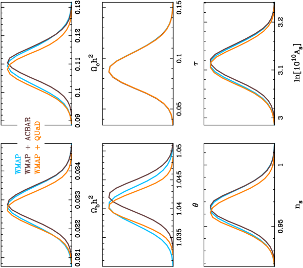
Figure 14.— 1D likelihood distribution for our base MCMC parameters for the basic 6-parameter $\Lambda$CDM model. The constraint on the scalar amplitude is presented at a pivot-point of $k^{s}_{\star}=0.013$ Mpc^-1.

The mean values of these parameters also shift a little but the only significant discrepancy is perhaps in the recovered value of $\theta$. Here, we find the WMAP + ACBAR combination prefers a somewhat higher value (in agreement with ACBAR’s own analysis; Reichardt et al. 2009) whereas the addition of QUaD data does not change the WMAP-only preferred mean value but simply tightens the constraint.

Note that in comparison to the WMAP team’s own analysis (Dunkley et al. 2009), we recover slightly different mean values for $\tau$ and more significantly different values for $z_{re}$. This is due to the different reionization model used in the later version of the CAMB software which we have used. We note in passing that the majority of the constraining power in the QUaD data comes from the measurements of the polarization power spectra as found with our previous analysis (Castro et al., 2009).

7.4. Running spectral index model

The 1D and 2D marginalized constraints on our base parameters for the running spectral index model, as obtained from our WMAP + QUaD runs are shown in Figure 15 along with the constraints using only the WMAP data. The recovered parameter values and their uncertainties are listed in Table 4.

The impact of QUaD data is greater for this model — the QUaD data adds significantly to the constraints on $\Omega_{b}h^{2}$, $\Omega_{c}h^{2}$, $\theta$, and $n_{\rm run}$, reducing the marginalized 1D errors on these parameters by up to $20\%$. Adding both the QUaD and ACBAR data has an even greater impact, reducing the errors on these parameters by up to a third compared to the WMAP-only uncertainties. Of particular interest are the constraints in the $n_{s}$ – $n_{\rm run}$ plane since many theories of inflation predict both a deviation from $n_{s}=1$ and/or a small negative running. Constraints from the WMAP + ACBAR + QUaD combination are shown in the left hand panel of Figure 16, together with the constraints from WMAP alone. Our 1D marginalized constraint on the running from the combined data set is $n_{\rm run}=0.046\pm 0.021$, $2.2\sigma$ away from the $n_{\rm run}=0$ model. Adding the LSS data to the mix improves the constraints even further, in our analysis tightening the $1\sigma$ error on $n_{\rm run}$ from 0.021 to 0.018. The significance of a non-zero running is also reduced on addition of the LSS data.

Comparing Tables 3 and 4, we see also that the 1D marginalized constraint on the spectral index, $n_{s}$ is not weakened by allowing a non-zero running. This is due to our use of the decorrelation pivot-scale as described in Section 7.2. The results also show that the constraints on $n_{s}$ obtained for the standard 6-parameter $\Lambda$CDM model are robust to marginalization over a possible running. For example, with the WMAP + ACBAR + QUaD combination, the constraint on $n_{s}$ goes from $n_{s}=0.962\pm 0.013$ to $n_{s}=0.965\pm 0.013$ when we allow for a possible non-zero running. For comparison, if instead, we use the WMAP-preferred pivot-point ($k^{s}_{\star}=0.002$ Mpc^-1), the marginalized 1D constraint on $n_{s}$ is degraded to $n_{s}=0.962\pm 0.019$ in the presence of running.

Hints of a negative running in the spectral index have been observed in previous CMB analyses (e.g. Dunkley et al. 2009; Reichardt et al. 2009). With the addition of the new QUaD data, this suggestion of a negative running not only persists, but is strengthened. We do, however, stress that the combined result shown in the left hand panel of Fig. 16 is still consistent with zero running at the $3\sigma$ level. Nevertheless, it is worth examining the implications for inflation models if the running was as large and as negative as the best-fit value returned from our analysis of the combined CMB data set. In this respect, Malquarti et al. (2004) have pointed out that an observed running of $n_{\rm run}\mathrel{\hbox to0.0pt{\lower 4.0pt\hbox{\hskip 1.0pt$\sim$}\hss}\raise 1.0pt\hbox{$<$}}-0.02$ would effectively rule out large field inflation models. More generally, Easther & Peiris (2006) have demonstrated that for a large negative running, single field slow roll inflation models will last less than 30 e-folds after entering the horizon. This amount of inflation is insufficient if inflation happened at the GUT scale. Consequently, an observation of $n_{\rm run}\sim-0.05$ would require inflation theory to move beyond the simplest models, e.g. by considering multiple fields and/or modifications to the slow-roll formalism (e.g. Chung et al. 2003; Makarov 2005; Ballesteros et al. 2006).

7.5. Tensor modes

Our constraints for the $\Lambda$CDM model including a possible tensor component are listed in Table 5 in terms of the mean recovered parameter values and their uncertainties. For $r$, we quote the 95% one-tail upper limit since as expected, no detection of tensors is made. For our WMAP-only analysis, we recover a slightly weaker limit ($r<0.48$) than that obtained by the WMAP team themselves ($r<0.43$; Dunkley et al. 2009). Adding either the ACBAR or QUaD data, this is reduced to $r<0.40$.

The WMAP + ACBAR + QUaD combination produces a constraint on tensor modes of $r<0.33$, the strongest from the CMB alone to date. Note that this constraint does not come from our upper limits on the $BB$ spectrum. It is, in fact, driven by a preference of the small-scale data (particularly the QUaD $EE$ and $TE$ data) for a somewhat lower spectral index compared to that preferred by WMAP alone — a lower $n_{s}$ allows more of the large-scale $TT$ power observed by WMAP to come from scalar perturbations and therefore the maximum allowed tensor contribution is reduced. Our CMB-only constraints in the $r$–$n_{s}$ plane are plotted in the right-hand panel of Figure 16.

Table 4 Parameter Constraints for the running spectral index model

	WMAP	WMAP+ACBAR	WMAP+QUaD	WMAP+ACBAR+QUaD	WMAP+ACBAR+QUaD+SDSS
$\Omega_{b}h^{2}$	$0.0221^{+0.0009}_{-0.0009}$	$0.0221^{+0.0007}_{-0.0007}$	$0.0219^{+0.0007}_{-0.0007}$	$0.0219^{+0.0006}_{-0.0006}$	$0.0223^{+0.0006}_{-0.0006}$
$\Omega_{c}h^{2}$	$0.116^{+0.009}_{-0.009}$	$0.120^{+0.008}_{-0.008}$	$0.117^{+0.008}_{-0.008}$	$0.120^{+0.008}_{-0.008}$	$0.111^{+0.004}_{-0.004}$
$\theta$	$1.0399^{+0.0030}_{-0.0031}$	$1.0414^{+0.0027}_{-0.0027}$	$1.0399^{+0.0024}_{-0.0024}$	$1.0409^{+0.0023}_{-0.0023}$	$1.0413^{+0.0022}_{-0.0022}$
$\tau$	$0.093^{+0.018}_{-0.018}$	$0.095^{+0.019}_{-0.019}$	$0.095^{+0.019}_{-0.018}$	$0.096^{+0.019}_{-0.019}$	$0.096^{+0.019}_{-0.018}$
$n_{s}$	$0.964^{+0.014}_{-0.014}$	$0.967^{+0.014}_{-0.014}$	$0.963^{+0.013}_{-0.013}$	$0.965^{+0.013}_{-0.013}$	$0.967^{+0.013}_{-0.013}$
$n_{\rm run}$	$-0.031^{+0.028}_{-0.028}$	$-0.040^{+0.023}_{-0.023}$	$-0.038^{+0.024}_{-0.024}$	$-0.046^{+0.021}_{-0.021}$	$-0.028^{+0.018}_{-0.018}$
${\cal A}_{s}$	$3.16^{+0.06}_{-0.06}$	$3.18^{+0.05}_{-0.05}$	$3.17^{+0.06}_{-0.06}$	$3.19^{+0.05}_{-0.05}$	$3.15^{+0.04}_{-0.04}$
$\Omega_{\Lambda}$	$0.70^{+0.05}_{-0.05}$	$0.69^{+0.05}_{-0.05}$	$0.70^{+0.05}_{-0.05}$	$0.69^{+0.05}_{-0.05}$	$0.74^{+0.02}_{-0.02}$
$Age$	$13.81^{+0.18}_{-0.18}$	$13.78^{+0.14}_{-0.15}$	$13.82^{+0.14}_{-0.14}$	$13.82^{+0.13}_{-0.13}$	$13.72^{+0.11}_{-0.11}$
$\Omega_{m}$	$0.30^{+0.05}_{-0.05}$	$0.31^{+0.05}_{-0.05}$	$0.30^{+0.05}_{-0.05}$	$0.31^{+0.05}_{-0.05}$	$0.26^{+0.02}_{-0.02}$
$\sigma_{8}$	$0.81^{+0.04}_{-0.04}$	$0.83^{+0.03}_{-0.03}$	$0.81^{+0.04}_{-0.04}$	$0.83^{+0.03}_{-0.03}$	$0.79^{+0.02}_{-0.02}$
$z_{re}$	$11.2^{+1.6}_{-1.6}$	$11.4^{+1.6}_{-1.6}$	$11.4^{+1.6}_{-1.6}$	$11.7^{+1.6}_{-1.6}$	$11.2^{+1.5}_{-1.5}$
$H_{0}$	$68.9^{+4.0}_{-4.0}$	$68.0^{+3.4}_{-3.4}$	$68.5^{+3.5}_{-3.6}$	$67.5^{+3.2}_{-3.2}$	$71.4^{+1.9}_{-1.9}$

Note. — The pivot point used for $\mathcal{A}_{s}$ and $n_{s}$ is $k^{s}_{\star}=0.013$ Mpc^-1.

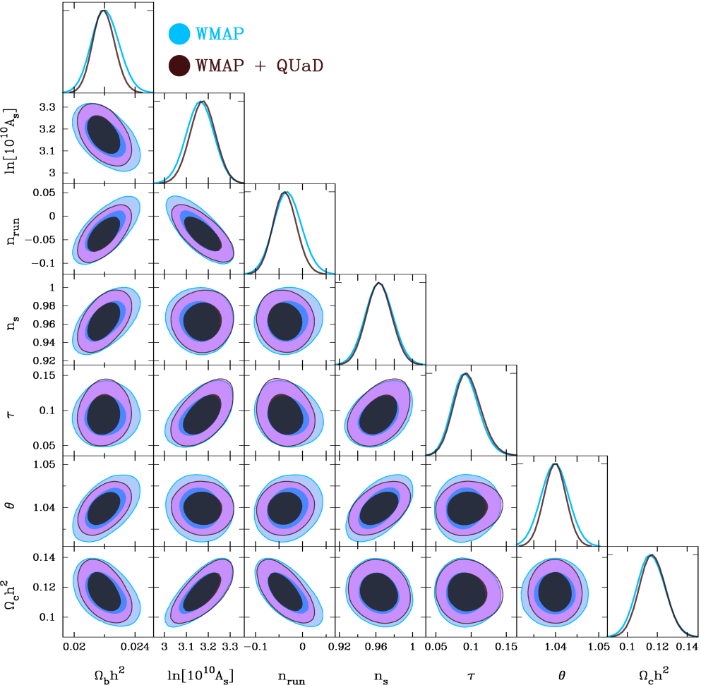
Figure 15.— 1D and 2D likelihood distributions recovered for the base MCMC parameters for the $\Lambda$CDM model extended to include a possible running in the scalar spectral index. The constraints on $n_{s}$ and $A_{s}$ are shown for the decorrelation pivot-point of $k^{s}_{\star}=0.013$ Mpc^-1. In the 2D panels, we indicate the regions of parameter space which enclose 68% and 95% of the likelihood as the inner and outer contours respectively. The results for the WMAP + QUaD combination are shown over-plotted on the WMAP-only results. Adding the QUaD data tightens the constraints on $\Omega_{b}h^{2}$, $\Omega_{c}h^{2}$, $n_{\rm run}$ and $\theta$ by up to $20\%$.

7.6. Running spectral index and tensor modes

When we allow for both a running in the spectral index and a tensor contribution the constraints weaken considerably versus either on their own. In the left-hand panel of Figure 17, for the WMAP + ACBAR + QUaD combination, we plot constraints in the $n_{\rm run}$–$n_{s}$ plane with and without marginalization over a possible tensor component. The right panel of this figure shows the corresponding constraints in the $r$–$n_{s}$ plane with and without marginalization over a possible running in the spectral index. For this model, the addition of QUaD and ACBAR data still improves the constraints in the spectral index running (and indeed, still strongly suggests a small negative running) but the constraints in the $r$–$n_{s}$ plane in the presence of running do not improve on the WMAP-only result. This degradation in the constraints on $r$ when we allow for a running in the spectral index is further demonstrated in Table 7.7 where we quote the 1D marginalized constraints on the parameters $\{r,n_{s}$, $n_{\rm run}\}$ for the tensors-only, running-only and tensors + running models. In this table, we present the results for the WMAP + ACBAR + QUaD combination and for the case where we add in the SDSS LRG data.

7.7. Constraints on parity violation

In the preceding sections, we used the QUaD $TT,EE,TE$ and $BB$ spectra to constrain the parameters of standard $\Lambda$CDM models and its usual extensions. For that analysis, we did not use our measurements of the cross-polarization spectrum ($EB$) or the correlation of temperature with $B$-modes ($TB$), since these spectra are expected to vanish in a universe which respects parity conservation (which the above models do). In this section, we use these two spectra (along with the $TE$, $EE$ and $BB$ measurements) to constrain a possible parity violation signal on cosmological scales. In the presence of parity violating interactions, a rotation in the polarization direction of CMB photons will be induced as they propagate from the surface of last scattering. If parity violating effects are present on cosmological scales, there will therefore be a net local rotation of the observed Stokes parameters, $Q$ and $U$ in the measured polarization map. This will mix $E$ and $B$ modes resulting in non-zero expectations for the $TB$ and $EB$ power spectra. Parametrizing the parity violation effect with a rotation angle, $\Delta\alpha$, the expectation values for the $TB$ and $EB$ spectra in terms of the cosmological $TE$ and $EE$ spectra are given by:

$$C_{\ell}^{TB} = C_{\ell}^{TE}\sin\,(2\Delta\alpha)$$ (31)

$$C_{\ell}^{EB} = \frac{1}{2}C_{\ell}^{EE}\sin\,(4\Delta\alpha)\,.$$ (32)

In addition, assuming that primordial and lensed $B$-modes are negligible (which is an excellent assumption given our sensitivity), the expectation value for the $BB$ spectrum is

$$C_{\ell}^{BB}=C_{\ell}^{EE}\sin^{2}(2\Delta\alpha)\,.$$ (33)

We used our previous results to place a constraint of $\Delta\alpha=0.53^{\circ}\pm 0.82^{\circ}\pm 0.50^{\circ}$ (Wu et al., 2009) where the two quoted uncertainties are the random and systematic components respectively.

Here, we repeat this analysis with our new measurements. The analysis is model-independent in the sense that we construct our estimator for $\Delta\alpha$ in terms of the observed power spectra and do not assume a cosmological model for the $EE$ or $TE$ signals. For details of our estimator and analysis (which has not changed since our previous work), we refer the reader to Wu et al. (2009).

We apply the estimator to the real QUaD data and assign error-bars due to random noise and sample variance by processing the suite of simulations containing both signal and noise through the analysis. The result is shown in Figure 18 where we plot both the results from simulations and from the real data. Note that our simulations contain no parity violating signals and so should scatter about zero, which they do. We take the scatter in the results from the simulations as our random error. Adding in the systematic error, our final result is

$$\Delta\alpha=0.64\pm 0.50\mbox{ (random)}\pm 0.50\mbox{ (systematic)}\,.$$ (34)

The random error has been reduced by $\sim 40\%$ with respect to our previous analysis in line with expectations.

Our result can be compared to the limits obtained from the WMAP 5-year data ($\Delta\alpha=-1.7\pm 2.1$; Komatsu et al. 2009) or to the limits obtained from the combination of the WMAP 5-year data and the B03 results ($\Delta\alpha=-2.6\pm 1.9$; Xia et al. 2008). We note that both of these quoted results include random errors only and do not include estimates of the systematic errors on the WMAP and B03 polarization calibration angles. Even when we include this systematic uncertainty for QUaD, our result is clearly a marked improvement over these previous analyses.

Table 5 Parameter constraints including a possible tensor component

	WMAP	WMAP+ACBAR	WMAP+QUaD	WMAP+ACBAR+QUaD	WMAP+ACBAR+QUaD+SDSS
$\Omega_{b}h^{2}$	$0.0235^{+0.0008}_{-0.0008}$	$0.0234^{+0.0007}_{-0.0007}$	$0.0232^{+0.0007}_{-0.0007}$	$0.0231^{+0.0006}_{-0.0006}$	$0.0229^{+0.0006}_{-0.0006}$
$\Omega_{c}h^{2}$	$0.104^{+0.007}_{-0.007}$	$0.106^{+0.007}_{-0.007}$	$0.103^{+0.007}_{-0.007}$	$0.105^{+0.006}_{-0.006}$	$0.107^{+0.004}_{-0.004}$
$\theta$	$1.0421^{+0.0033}_{-0.0033}$	$1.0433^{+0.0028}_{-0.0028}$	$1.0412^{+0.0026}_{-0.0026}$	$1.0423^{+0.0023}_{-0.0023}$	$1.0419^{+0.0022}_{-0.0023}$
$\tau$	$0.094^{+0.018}_{-0.018}$	$0.092^{+0.018}_{-0.018}$	$0.093^{+0.018}_{-0.018}$	$0.091^{+0.017}_{-0.017}$	$0.088^{+0.017}_{-0.017}$
$n_{s}$	$0.990^{+0.023}_{-0.023}$	$0.986^{+0.021}_{-0.020}$	$0.982^{+0.020}_{-0.020}$	$0.978^{+0.018}_{-0.018}$	$0.973^{+0.015}_{-0.015}$
${\cal A}_{s}$	$3.07^{+0.05}_{-0.05}$	$3.08^{+0.04}_{-0.04}$	$3.08^{+0.04}_{-0.04}$	$3.09^{+0.04}_{-0.04}$	$3.09^{+0.03}_{-0.04}$
$r$	$<0.48$ (95% c.l.)	$<0.40$ (95% c.l.)	$<0.40$ (95% c.l.)	$<0.33$ (95% c.l.)	$<0.27$ (95% c.l.)
$\Omega_{\Lambda}$	$0.78^{+0.03}_{-0.03}$	$0.77^{+0.03}_{-0.03}$	$0.78^{+0.03}_{-0.03}$	$0.77^{+0.03}_{-0.03}$	$0.76^{+0.02}_{-0.02}$
$Age$	$13.52^{+0.18}_{-0.18}$	$13.51^{+0.16}_{-0.16}$	$13.57^{+0.15}_{-0.15}$	$13.57^{+0.13}_{-0.13}$	$13.61^{+0.11}_{-0.11}$
$\Omega_{m}$	$0.22^{+0.03}_{-0.03}$	$0.23^{+0.03}_{-0.03}$	$0.22^{+0.03}_{-0.03}$	$0.23^{+0.03}_{-0.03}$	$0.24^{+0.02}_{-0.02}$
$\sigma_{8}$	$0.77^{+0.04}_{-0.04}$	$0.78^{+0.04}_{-0.04}$	$0.76^{+0.04}_{-0.04}$	$0.78^{+0.03}_{-0.03}$	$0.78^{+0.02}_{-0.02}$
$z_{re}$	$10.5^{+1.4}_{-1.4}$	$10.5^{+1.4}_{-1.4}$	$10.5^{+1.4}_{-1.3}$	$10.4^{+1.4}_{-1.3}$	$10.3^{+1.3}_{-1.3}$
$H_{0}$	$75.8^{+3.8}_{-3.8}$	$75.2^{+3.4}_{-3.4}$	$75.5^{+3.4}_{-3.4}$	$74.8^{+3.1}_{-3.1}$	$73.8^{+1.8}_{-1.9}$

Note. — The pivot point used for $\mathcal{A}_{s}$ is $k^{s}_{\star}=0.013$ Mpc^-1 while the pivot point used for the tensor-to-scalar ratio, $r$ is $k^{t}_{\star}=0.002$ Mpc^-1.

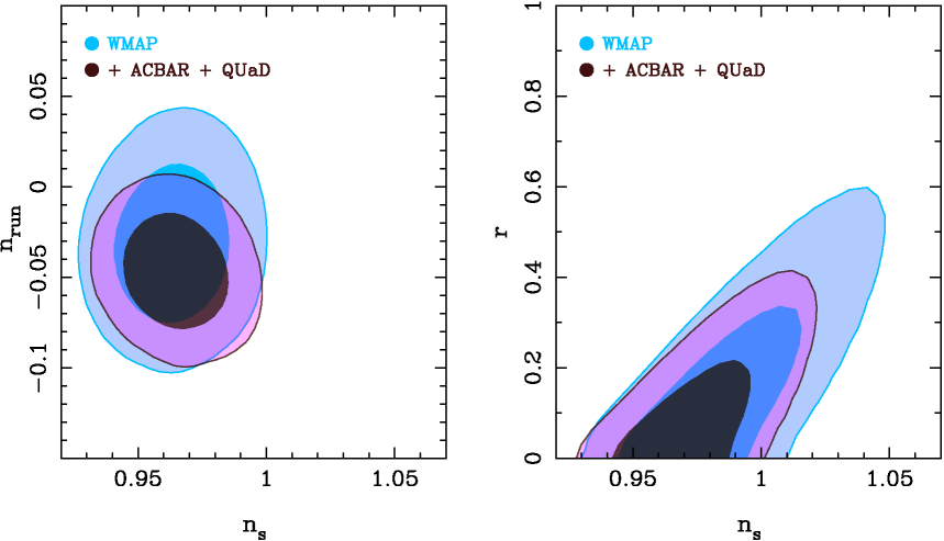
Figure 16.— Left panel: 68% and 95% confidence regions in the $n_{s}$-$n_{\rm run}$ plane, marginalised over all other parameters, for the WMAP + ACBAR + QUaD combination as compared to those obtained from WMAP alone. The constraints are shown for a pivot-point of $k^{s}_{\star}=0.013$ Mpc^-1. No tensor component was allowed for either set of constraints. The constraints tighten by about one third. The mean recovered values also shift further away from the simple $\{n_{s},n_{\rm run}\}=\{1,0\}$ model. Right panel: Marginalized constraints on the inflation parameters, $r$ and $n_{s}$ from WMAP data alone and adding in the ACBAR and QUaD datasets. No running in the spectral index was allowed for these fits and the tensor-to-scalar ratio, $r$ is presented for a tensor pivot-point of $k^{t}_{\star}=0.002$ Mpc^-1. Once again, the inner and outer contours indicate the regions of parameter space enclosing 68% and 95% of the likelhood respectively. The 95% upper limit on $r$ is reduced from $r<0.48$ to $r<0.33$. This constraint is driven by the preference of the additional datasets for a lower spectral index than is recovered from the WMAP data on its own.

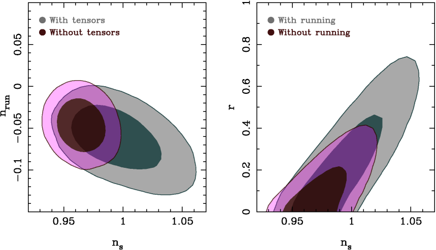
Figure 17.— Left panel: Constraints are shown (as 68% and 95% confidence regions) in the $n_{\rm run}$–$n_{s}$ plane with and without marginalization over a possible tensor component. These fits are for the WMAP + ACBAR + QUaD combination. Allowing a non-zero tensor component weakens the constraints considerably. However, the addition of both QUaD and ACBAR to WMAP still favors a small negative running. Right panel: The 68% and 95% central confidence regions in the $r$–$n_{s}$ plane (for WMAP + ACBAR + QUaD) with and without marginalization over a possible running in the spectral index. Allowing the spectral index to run degrades the constraints to such an extent that the addition of QUaD and/or ACBAR data yields no improvement over the WMAP-only constraints. $n_{s}$ is evaluated at $k^{s}_{\star}=0.013$ Mpc^-1 (for both panels) and $r$ is evaluated at $k^{t}_{\star}=0.002$ Mpc^-1.

Table 6Constraints on inflationary parameters

Figure 18.— Constraints on possible parity violation interactions on cosmological scales, parametrized in terms of the parity violation rotation angle, $\Delta\alpha$. The histogram shows the estimates of $\Delta\alpha$ as measured from our suite of signal + noise simulations. The vertical red line shows $\Delta\alpha$ as measured from the real QUaD data. The full and dashed blue lines show the 68% and 95% confidence regions about the central value as estimated from the scatter in the simulation results.

7.8. Limits on the lensed $B$-mode signal

Although QUaD has not made any detection of $B$-modes, it is the most sensitive small-scale CMB polarization experiment to date. We can therefore place the leading upper limit on the presence of a small scale $B$-mode signal. The signal expected to dominate on the scales at which QUaD is sensitive is that induced by gravitational lensing of $E$-modes by intervening large scale structure. As well as measuring cosmological $B$-modes from inflation, future polarization experiments will target this lensing signal from which useful information can be gained on dark energy and massive neutrinos (e.g. Kaplinghat et al. 2003; Smith et al. 2006).

Assuming a single flat band power between $\ell=200$ and $\ell=2000$, we find $\ell(\ell+1)C^{BB}_{\ell}/2\pi=0.17\pm 0.17\,\mu{\rm K}^{2}$ with a 95% upper limit of $0.57\,\mu{\rm K}^{2}$. The errors quoted are estimated from the scatter in the results obtained from the suite of simulations containing both signal and noise. For comparison, the $\Lambda$CDM expectation value for this band power is $0.058\,\mu{\rm K}^{2}$. Alternatively, assuming the $\Lambda$CDM shape for the lensing signal, and simply fitting for its amplitude between $\ell=200$ and $\ell=2000$, our constraint on the amplitude is $2.5\pm 4.5$ with a 95% upper limit of $12.5$.

Note that although we have used all of our $BB$ band powers to obtain the above constraints, the window function of our estimator is strongly skewed towards lower multipoles where the band power uncertainties are much smaller. The effective range of multipoles to which our upper limits apply is, in fact, $170<\ell<400$ rather than the nominal $200<\ell<2000$ range.

Although our $2\sigma$ upper limits are an order of magnitude larger than the expected $\Lambda$CDM signal, they are, in turn, roughly an order of magnitude better than previously reported limits on the amplitude of the $B$-mode signal in this angular scale range.

8. Conclusions

We have presented a re-analysis of the final dataset from the QUaD experiment, a CMB polarimeter which observed the CMB at 100 and 150 GHz from the South Pole between 2005 and 2007. A major part of this re-analysis was the development of a new technique for removing ground contamination from the data. The ground signal seen in QUaD data is polarized and, if not removed, contaminates all of the CMB power spectrum measurements. Our new procedure, which is based on constructing, and subsequently subtracting, templates of the ground signal has allowed us to reconstruct maps of the $T$, $Q$ and $U$ Stokes parameters over the full sky area. Although the method is not entirely lossless, it provides, on average, a 30% increase in the precision of the power spectra compared to our previous analysis which used field-differencing to remove the ground.

Through further detailed analysis of calibration data, we have also significantly improved our understanding of the QUaD beams. We have implemented new beam models which explicitly incorporate the effects of sidelobes, resulting in an increase of $\sim 10\%$ in the amplitude of our power spectra measurements for multipoles, $\ell\mathrel{\hbox to0.0pt{\lower 4.0pt\hbox{\hskip 1.0pt$\sim$}\hss}\raise 1.0pt\hbox{$>$}}700$. The shift in power is most relevant for our high-$\ell$ temperature power spectrum measurements where the signal-to-noise is high.

We have presented results using our two independent analysis pipelines. Though there are significant differences in the approach between the two pipelines, the final results agree very well. Testing the power spectra against the best-fit $\Lambda$CDM model to the WMAP 5-year data, we find good agreement. Our measurements of the $E$-mode polarization spectrum, and of the cross-correlation between the $E$-modes and the CMB temperature field, are the most precise at multipoles $\ell>200$ to date. Our measurement of the temperature power spectrum at $\ell>1000$ is among the best constraints on temperature anisotropies on small angular scales and is competitive with the final ACBAR result (Reichardt et al., 2009).

We have subjected our results to the same set of rigorous jackknife tests for systematic effects as was performed in our previous analysis (Pryke et al., 2009). We find no evidence for residual systematic effects in our polarization maps. Although formally, many of our $TT$ jackknife tests fail, the inferred levels of residual systematics are negligible compared to our sample-variance driven error bars. Moreover, the very small level of power seen in our frequency difference maps and power spectra indicate that foreground contamination is also negligible compared to our uncertainties.

We have used our power spectra measurements, in combination with the WMAP 5-year results and the ACBAR results to place constraints on the parameters of cosmological models. For the standard 6-parameter $\Lambda$CDM model, the QUaD data adds only marginally to the constraints obtained from the WMAP data alone. The impact of the QUaD data is greater in a model extended to include a running in the spectral index, reducing the uncertainties in $\Omega_{b}h^{2}$, $\Omega_{c}h^{2}$, $\theta$ and $n_{\rm run}$ by up to 20%. The addition of both QUaD and ACBAR data is more powerful still, improving the constraints on these four parameters by up to one third. For a $\Lambda$CDM model extended to include a possible tensor component, we find that the addition of both ACBAR and QUaD data reduces the upper limit on the tensor-to-scalar ratio from $r<0.48$ to $r<0.33$ (95% c.l.). This is the strongest limit to date on tensors from the CMB alone. The improvement is driven by a tendency of the QUaD data to prefer a somewhat smaller spectral index than is inferred from WMAP data alone.

We have used our measurements of the $TB$ and $EB$ power spectra to put constraints on possible parity-violating interactions on cosmological scales. Following our previous analysis (Wu et al., 2009), we constrain the rotation angle due to such a possible “cosmological birefringence” to be $0.64^{\circ}\pm 0.50^{\circ}\pm 0.50^{\circ}$ where the errors quoted are the random and systematic contributions. Our result is equivalent to a constraint on isotropic Lorentz-violating interactions of $k^{(3)}_{(V)00}<1.5\times 10^{-43}$ GeV (68% c.l.).

Finally, we have placed an upper limit on the strength of the lensing $B$-mode signal using our measurements of the $BB$ power spectrum. Assuming the concordance $\Lambda$CDM shape for lensing $B$-modes, we constrain its amplitude (where the normalization is such that the $\Lambda$CDM model has amplitude $=1$) to be $2.5\pm 4.5$ with a 95% upper limit of 12.5. Alternatively, assuming a single flat band power for $\ell>200$ we find a 95% upper limit of $\ell(\ell+1)C^{BB}_{\ell}/2\pi<0.57\,\mu{\rm K}^{2}$ for the amplitude of $B$-modes.

Appendix A Beam uncertainties

As described in Section 4, our new beam models involve either fitting the QUaD physical optics (PO) beam models to QSO data (Pipeline 1) or measuring the sidelobes directly from QSO maps under the assumption that the sidelobes are azimuthally symmetric (Pipeline 2). Although the predicted radially averaged beam profiles from both of these approaches appear to match the data very well, the fits are not perfect and are subject to an uncertainty in the sidelobe levels. There is also an uncertainty on the width of the main lobe, dominated by small temperature-dependent variations. Based on the fluctuations in the beam widths seen in our “rowcal” data, we estimate the remaining uncertainty on the main lobe width to be 2.5% of the effective FWHMs of 5.2 and 3.8 arcmin at 100 GHz and 150 GHz respectively. We obtain the uncertainty on the level of our sidelobes from the errors returned from fitting our PO simulations to the QSO observations in Pipeline 1.

To propagate these errors onto uncertainties in the transfer functions of Section 6.3, for the error in the main lobe, we simply note that the effect of a fractional error, $\delta$ in the FWHM of a Gaussian beam is well approximated by

$$\frac{\Delta B^{2}_{\ell}}{B^{2}_{\ell}}\,=\,\exp\left[\sigma^{2}_{b}(\delta^{2}+2\delta)\ell(\ell+1)\right]\,-\,1\,,$$ (A1)

where $\sigma_{b}=\theta_{\rm FWHM}/\sqrt{8\ln 2}$ is the beam width. For the errors in the sidelobes, we take the minimum and maximum sidelobe levels as returned from the fits of the PO models to the data, coadd the resulting beam models across detectors and radially average to produce the minimum and maximum allowed radial profiles, $B(\theta)$, for each frequency. Taking the Legendre transform of these profiles,

$$B_{\ell}=2\pi\int B(\theta)P_{\ell}\cos(\theta)\,d\!\cos(\theta)\,,$$ (A2)

we estimate the error in our beam transfer functions due to the uncertainty in the sidelobes as

$$\Delta B^{2}_{\ell}=B_{{\rm max},\ell}^{2}-B_{{\rm min},\ell}^{2}\,.$$ (A3)

We take the quadrature sum of the errors due to the main lobe and sidelobe uncertainties to be the final error. These uncertainties are shown in Figure 19 along with the quadrature sum. Since our combined spectra are dominated by the 150 GHz channel, the curves for the combined spectra are approximately the same as the 150 GHz curves.

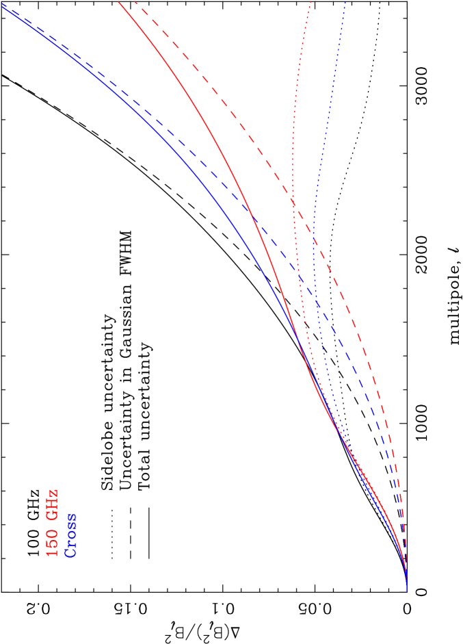
Figure 19.— Fractional uncertainties on our beam transfer functions. The dashed curves show the errors due to the 2.5% uncertainty in the width of the main lobe beams. The dotted curves show the sidelobe uncertainties and the full curves show the total uncertainties. The corresponding curves for the combined spectra are similar to the 150 GHz curves shown in red. At 150 GHz, the uncertainty in the level of the sidelobes dominates the beam uncertainty for the full $\ell$-range presented in this paper.

Appendix B Absolute calibration uncertainty

As described in Section 5, our calibration is performed by taking the ratio of cross-spectra between the QUaD and B03 temperature maps. This process is subject to several uncertainties.

Firstly, there is a statistical error in the calibration ratio, predominantly due to noise in the B03 maps. To estimate this error, we perform Monte-Carlo simulations of the absolute calibration process. Assuming white noise and a $\Lambda$CDM power spectrum, we use the B03 hit-maps along with their stated sensitivities to produce simulations of the B03 maps. We do the same thing for QUaD and apply a known $\mu$K $\rightarrow$ V calibration to the simulated QUaD maps. Each pair of simulated maps is then passed through the absolute calibration analysis. The scatter in the calibration factors recovered from these simulations is 0.6% and we take this as the statistical uncertainty in our calibration.

Our calibration ratio as a function of multipole is not perfectly flat but fluctuates about a mean value. Although some of this scatter will be due to noise (which is included in our estimate of the statistical error), we conservatively also include this scatter, which we measure to be 1.1%, in our error budget. In addition, we have also performed the calibration analysis using each of the jackknife splits described in Section 6.5. Although the scatter found in the recovered calibration numbers do not indicate any significant inconsistencies, we also include this scatter in our error budget.

To propagate the errors in the B03 and QUaD beam transfer functions onto our calibration, we repeat the analysis but with the beam functions shifted by their quoted errors. Doing this for each of the B03 and QUaD beams, we take the resulting shifts in the calibration numbers as the error due to uncertainty in the beams. We find a 1.1% shift due to the uncertainty in the B03 beam function and a 0.75% shift due to the uncertainty in QUaD’s beam.

A further source of error is the relative pointing uncertainty between the QUaD and B03 maps. There is a clear pointing offset seen between the QUaD and B03 maps and so we have shifted the B03 maps before performing the calibration analysis. We find the appropriate shift (which we model as a simple shift in R.A. and Dec) by fitting for it in map-space. To quantify the error, we repeat the analysis with the B03 maps shifted (away from the best fit) according to the errors returned from our map-based fit. Applying the shift in a number of different directions (the eight compass points), we find the maximum shift in the resulting calibration factor is 1.6%. We take this number as our error due to the B03/QUaD relative pointing uncertainty.

Finally, QUaD also inherits the stated uncertainty in the B03 calibration which is 2% (Masi et al. 2006). We add this and each of the errors derived above in quadrature to arrive at our final calibration uncertainty of 3.4%. Our absolute calibration error budget is summarized in Table B.

Table 7Absolute calibration uncertainties for QUaD

References

- Ade et al. (2008) Ade, P. et al. 2008, ApJ, 674, 22
- Ballesteros et al. (2006) Ballesteros, G., Casas, J. A., & Espinosa, J. R. 2006, J. Cosmology Astropart. Phys, 3, 1
- Barkats et al. (2005) Barkats, D. et al. 2005, ApJ, 619, L127
- Bennett et al. (2003) Bennett, C. L. et al. 2003, ApJS, 148, 1
- Bischoff et al. (2008) Bischoff, C. et al. 2008, ApJ, 684, 771
- Bond et al. (2000) Bond, J. R., Jaffe, A. H., & Knox, L. 2000, ApJ, 533, 19
- Brown et al. (2005) Brown, M. L., Castro, P. G., & Taylor, A. N. 2005, MNRAS, 360, 1262
- Castro et al. (2009) Castro, P. G. et al. 2009, ApJ, 701, 857
- Challinor & Peiris (2009) Challinor, A., & Peiris, H. 2009, ArXiv e-prints, 0903.5158
- Chiang et al. (2009) Chiang, H. C. et al. 2009, ArXiv e-prints, 0906.1181
- Chung et al. (2003) Chung, D. J., Shiu, G., & Trodden, M. 2003, Phys. Rev. D, 68, 063501
- Copeland et al. (1998) Copeland, E. J., Grivell, I. J., & Liddle, A. R. 1998, MNRAS, 298, 1233
- Cortês et al. (2007) Cortês, M., Liddle, A. R., & Mukherjee, P. 2007, Phys. Rev. D, 75, 083520
- Dunkley et al. (2009) Dunkley, J. et al. 2009, ApJS, 180, 306
- Easther & Peiris (2006) Easther, R., & Peiris, H. V. 2006, J. Cosmology Astropart. Phys, 9, 10
- Ferreira & Jaffe (2000) Ferreira, P. G., & Jaffe, A. H. 2000, MNRAS, 312, 89
- Finelli et al. (2006) Finelli, F., Rianna, M., & Mandolesi, N. 2006, J. Cosmology Astropart. Phys, 12, 6
- Friedman et al. (2009) Friedman, R. B. et al. 2009, ApJ, 700, L187
- Frigo & Johnson (2005) Frigo, M., & Johnson, S. G. 2005, Proceedings of the IEEE, 93, 216, special issue on ”Program Generation, Optimization, and Platform Adaptation”
- Górski et al. (2005) Górski, K. M., Hivon, E., Banday, A. J., Wandelt, B. D., Hansen, F. K., Reinecke, M., & Bartelmann, M. 2005, ApJ, 622, 759
- Hinderks et al. (2009) Hinderks, J. R. et al. 2009, ApJ, 692, 1221
- Hinshaw et al. (2009) Hinshaw, G. et al. 2009, ApJS, 180, 225
- Hivon et al. (2002) Hivon, E., Górski, K. M., Netterfield, C. B., Crill, B. P., Prunet, S., & Hansen, F. 2002, ApJ, 567, 2
- Kaplinghat et al. (2003) Kaplinghat, M., Knox, L., & Song, Y.-S. 2003, Phys. Rev. Lett., 91, 241301
- Knox (1999) Knox, L. 1999, Phys. Rev. D, 60, 103516
- Komatsu et al. (2009) Komatsu, E. et al. 2009, ApJS, 180, 330
- Komatsu & Seljak (2002) Komatsu, E., & Seljak, U. 2002, MNRAS, 336, 1256
- Kovac et al. (2002) Kovac, J. M., Leitch, E. M., Pryke, C., Carlstrom, J. E., Halverson, N. W., & Holzapfel, W. L. 2002, Nature, 420, 772
- Leitch et al. (2005) Leitch, E. M., Kovac, J. M., Halverson, N. W., Carlstrom, J. E., Pryke, C., & Smith, M. W. E. 2005, ApJ, 624, 10
- Lewis (2008) Lewis, A. 2008, Phys. Rev. D, 78, 023002
- Lewis & Bridle (2002) Lewis, A., & Bridle, S. 2002, Phys. Rev. D, 66, 103511
- Lewis et al. (2000) Lewis, A., Challinor, A., & Lasenby, A. 2000, ApJ, 538, 473
- Lidsey et al. (1997) Lidsey, J. E., Liddle, A. R., Kolb, E. W., Copeland, E. J., Barreiro, T., & Abney, M. 1997, Reviews of Modern Physics, 69, 373
- Lue et al. (1999) Lue, A., Wang, L., & Kamionkowski, M. 1999, Phys. Rev. Lett., 83, 1506
- Makarov (2005) Makarov, A. 2005, Phys. Rev. D, 72, 083517
- Malquarti et al. (2004) Malquarti, M., Leach, S. M., & Liddle, A. R. 2004, Phys. Rev. D, 69, 063505
- Masi et al. (2006) Masi, S. et al. 2006, A&A, 458, 687
- Montroy et al. (2006) Montroy, T. E. et al. 2006, ApJ, 647, 813
- Nolta et al. (2009) Nolta, M. R. et al. 2009, ApJS, 180, 296
- O’Sullivan et al. (2008) O’Sullivan, C. et al. 2008, Infrared Physics and Technology, 51, 277
- Page et al. (2007) Page, L. et al. 2007, ApJS, 170, 335
- Peiris & Easther (2006) Peiris, H. V., & Easther, R. 2006, J. Cosmology Astropart. Phys, 10, 17
- Piacentini et al. (2006) Piacentini, F. et al. 2006, ApJ, 647, 833
- Pryke et al. (2009) Pryke, C. et al. 2009, ApJ, 692, 1247
- Readhead et al. (2004) Readhead, A. C. S. et al. 2004, Science, 306, 836
- Reichardt et al. (2009) Reichardt, C. L. et al. 2009, ApJ, 694, 1200
- Sievers et al. (2007) Sievers, J. L. et al. 2007, ApJ, 660, 976
- Smith et al. (2006) Smith, S., Challinor, A., & Rocha, G. 2006, Phys. Rev. D, 73, 023517
- Stompor et al. (2002) Stompor, R. et al. 2002, Phys. Rev. D, 65, 022003
- Tegmark et al. (2006) Tegmark, M. et al. 2006, Phys. Rev. D, 74, 123507
- Wu et al. (2009) Wu, E. Y. S. et al. 2009, Phys. Rev. Lett., 102, 161302
- Wu et al. (2007) Wu, J. H. P. et al. 2007, ApJ, 665, 55
- Xia et al. (2008) Xia, J.-Q., Li, H., Zhao, G.-B., & Zhang, X. 2008, ApJ, 679, L61