Prospects for GRB science with the $Fermi$ Large Area Telescope

Abstract

The LAT instrument on the $Fermi$ mission will reveal the rich spectral and temporal gamma-ray burst phenomena in the $>$100 MeV band. The synergy with $Fermi$’s GBM detectors will link these observations to those in the well-explored 10–1000 keV range; the addition of the $>$100 MeV band observations will resolve theoretical uncertainties about burst emission in both the prompt and afterglow phases. Trigger algorithms will be applied to the LAT data both onboard the spacecraft and on the ground. The sensitivity of these triggers will differ because of the available computing resources onboard and on the ground. Here we present the LAT’s burst detection methodologies and the instrument’s GRB capabilities.

1 Introduction

The Large Area Telescope (LAT) on the $Fermi$ Gamma-ray Space Telescope (formerly GLAST—Gamma-ray Large Area Space Telescope) will turn the study of the 20 MeV to more than 300 GeV spectral and temporal behavior of gamma-ray bursts (GRBs) from speculation based on a few suggestive observations to a decisive diagnostic of the emission processes. The burst observations of the Energetic Gamma-Ray Experiment Telescope (EGRET) on the Compton Gamma-Ray Observatory (CGRO) suggested three types of high energy emission: an extrapolation of the 10–1000 keV spectral component to the $>$100 MeV band; an additional spectral component during the $<$1 MeV ‘prompt’ emission; and high energy emission that lingers long after the prompt emission has faded away. The LAT’s observations, in conjunction with the Gamma-ray Burst Monitor (GBM—8 keV to 30 MeV), will provide unprecedented spectral-temporal coverage for a large number of bursts. The spectra from these two instruments will cover seven and a half energy decades ($<$10 keV to $>$300 GeV; see Fig. 1, which shows different theoretically-predicted spectra). Thus the LAT will explore the rich phenomena suggested by the EGRET observations, probing the physical processes in the extreme radiating regions.

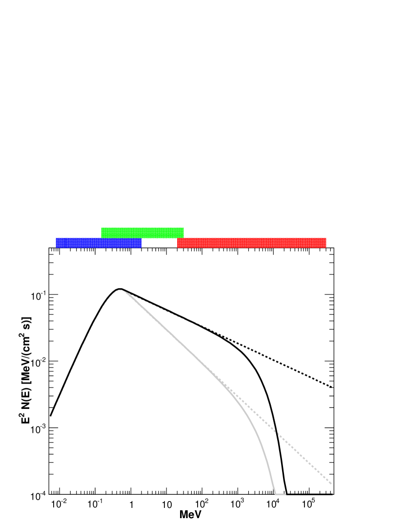
Figure 1: Simulated gamma-ray burst spectra, showing the broad energy range covered by $Fermi$: (from left to right) the GBM NaI (blue band: 8–2000 keV), the GBM BGO (green: 150 keV–30 MeV) and the LAT (red curve: 20 MeV to $>$300 GeV) detectors. The dashed curves are simple extrapolations of the typical GRB 10–1000 keV spectra into the GeV band, while the solid curves add an exponential cutoff that might result from absorption internal or external to the burst. The two different high energy photon indices $\beta$=-2.25 (black curves) and $\beta$=-2.5 (grey curves) demonstrate the dependence of the expected LAT flux on this photon index. There may be additional high energy components that are not known yet and are not shown in the figure.

In this paper we provide the scientific community interested in GRBs with an overview of the LAT’s operations and capabilities in this research area. Our development of detection and analysis tools has been guided by the previous observations and the theoretical expectations for emission in the $>$100 MeV band (§ 2). The LAT is described in depth in an instrument paper(Atwood et al., 2009), and therefore here we only provide a brief summary of the $Fermi$ mission and the LAT, focusing on issues relevant to burst detection and analysis (§ 3). Simulations are the basis of our analysis of the mission’s burst sensitivity, and are largely based on CGRO observations (§ 4). We use our simulation methodology to estimate the ultimate burst sensitivity and the resulting burst flux distribution (§ 5). Both the LAT and the GBM will apply burst detection algorithms onboard and on the ground, and the efficiency of these methods will determine which bursts the LAT will detect, and with what latency (§ 6). Once a burst has been detected, spectral and temporal analysis of LAT (and GBM) data will be possible (§ 7). The burst observations by ground-based telescopes and other space missions, particularly Swift, will complement the $Fermi$ observations (§ 8). While basic methods are in place for detecting and analyzing burst data, in-flight experience will guide future work (§ 9).

2 Burst Physics Above 100 MeV

2.1 Previous Observations

The detectors of the Compton Gamma-Ray Observatory (CGRO) provided time-resolved spectra for a statistically well-defined burst population. These observations are the foundation of our expectations for $Fermi$’s discoveries, which have guided the development of analysis tools before launch.

The Burst And Transient Source Experiment (BATSE) on CGRO observed a large sample of bursts in the $\sim$25–2000 keV band with well-understood population statistics (Paciesas et al., 1999). Spectroscopy by the BATSE detectors found that the emission in this energy band could be described by the empirical four parameter “Band” function (Band et al., 1993)

$$N_{\rm Band}(E|N_{0},E_{p},\alpha,\beta)=N_{0}\left\{\begin{array}[]{l l}E^{\alpha}\exp[-E(2+\alpha)/E_{p}],&E\leq{{\alpha-\beta}\over{2+\alpha}}E_{p}\\ \\ E^{\beta}\left[{{\alpha-\beta}\over{2+\alpha}}E_{p}\right]^{(\alpha-\beta)}\exp[\beta-\alpha],&E>{{\alpha-\beta}\over{2+\alpha}}E_{p},\end{array}\right.$$ (1)

where $\alpha$ and $\beta$ are the low and high energy photon indices, respectively, and $E_{p}$ is the ‘peak energy’ which corresponds to the maximum of $E^{2}N(E)\propto\nu f_{\nu}$ for the low energy component. Typically $\alpha\sim-0.5$ to $-1$ and $\beta$ is less than $-2$ (Band et al., 1993; Preece et al., 2000; Kaneko et al., 2006); the total energy would be infinite if $\beta\geq-2$ unless the spectrum has a high energy cutoff. The observations of 37 bursts by the Compton Telescope (COMPTEL) on CGRO (0.75–30 MeV) are consistent with the BATSE observations of this spectral component (Hoover et al., 2005). Because of the relatively poor spectral resolution of the BATSE detectors (Briggs, 1999), this functional form usually is a good description of spectra accumulated over both short time periods and entire bursts, even though bursts show strong spectral evolution (Ford et al., 1995). It is this 10–1000 keV ‘prompt’ component that is well-characterized and therefore provides a basis for quantitative predictions. A detailed duration-integrated spectral analysis (in  30 keV-200 MeV) of the prompt emission for 15 bright BATSE GRB performed by Kaneko et al. (2008) confirmed that only in few case there’s a significant high-energy excess with respect to low energy spectral extrapolations.

The burst observations by the Energetic Gamma-Ray Experiment Telescope (EGRET) on CGRO (20 MeV to 30 GeV) provide the best prediction of the LAT observations. EGRET observed different types of high energy burst phenomena. Four bursts had simultaneous emission in both the EGRET and BATSE energy bands, suggesting that the spectrum observed by BATSE extrapolates to the EGRET energy band (Dingus, 2003). However, the correlation with the prompt phase pulses was hampered by the severe EGRET spark chamber dead time ($\sim$100 ms/event) that was comparable or longer than the pulse timescales. The EGRET observations of these bursts suggest that the $\sim$1 GeV emission often lasts longer than the lower energy emission, and thus results in part from a different physical origin. A similar behaviour is present also in GRB 080514B detected by AGILE(Giuliani et al., 2008).

Whether high energy emission is present in both long and short bursts is unknown. The four bursts with high energy emission detected by EGRET were all long bursts, although GRB 930131 is an interesting case. It was detected by BATSE (Kouveliotou et al., 1994) with duration of $T_{90}$=14 s and found to have high-energy ($>$30 MeV) photons accompanying the prompt phase and possibly extending beyond (Sommer et al., 1994). The BATSE lightcurve is dominated by a hard initial emission lasting  1 sec and followed by a smooth extended emission. This burst may, therefore, have been one of those long bursts possibly associated with a merger and not a collapsar origin, commonly understood as the most probable origin for short and long burst respectively(Zhang, 2007). Several events have now been identified that could fit into this category (Norris & Bonnell, 2006) and their origin is still uncertain. LAT will make an important contribution in determining the nature of the high energy emission from similar events and a larger sample of bursts with detected high energy emission will determine whether the absence of high energy emission differentiates short from long bursts.

A high energy temporally resolved spectral component in addition to the Band function is clearly present in GRB 941017 (González et al., 2003); this component is harder than the low energy prompt component, and continues after the low energy component fades into the background. The time integrated spectra of both GRB 941017 and GRB 980923 show this additional spectral component (Kaneko et al., 2008).

Finally, the $>$1 GeV emission lingered for 90 minutes after the prompt low energy emission for GRB 940217, including an 18 GeV photon 1.5 hours after the burst trigger (Hurley et al., 1994). Whether this emission is physically associated with the lower energy afterglows is unknown.

These three empirical types of high energy emission—an extrapolation of the low energy spectra; an additional spectral component during the low energy prompt emission; and an afterglow—guide us in evaluating $Fermi$’s burst observation capabilities.

Because the prompt low energy component was characterized quantitatively by the BATSE observations while the EGRET observations merely demonstrated that different components were present, our simulations are based primarily on extrapolations of the prompt low energy component from the BATSE band to the $>$100 MeV band. We recognize that the LAT will probably detect additional spectral and temporal components, or spectral cutoffs, that are not treated in this extrapolation.

During the first few months of the $Fermi$ mission, LAT detected already emission from three GRBs: 080825C (Bouvier et al., 2008), 080916C (Tajima et al., 2008) and 081024B (Omodei, 2008). The rich phenomenology of high energy emission is confirmed in these three events, where spectral measurements over various order of magnitude were possible together with the detection of extended emission and spectral lags. In particular, the GRB 080916C was bright enough to afford unprecedented broad-band spectral coverage in four distinct time intervals (Abdo et al., 2009), thereby offering new insights into the character of energetic bursts.

2.2 Theoretical Expectations

In the current standard scenario, the burst emission arises in a highly relativistic, unsteady outflow. Several different progenitor types could create this outflow, but the initial high optical depth within the outflow obscures the progenitor type. As this outflow gradually becomes optically thin, dissipation processes within the outflow, as well as interactions with the surrounding medium, cause particles to be accelerated to high energies and loose some of their energy into radiation. Magnetic fields at the emission site can be strong and may be caused by a frozen-in component carried out by the outflow from the progenitor, or may be built up by turbulence or collisionless shocks. The emitted spectral distribution then depends on the details of the radiation mechanism, particle acceleration, and the dynamics of the explosion itself.

‘Internal shocks’ result when a faster region catches up with a slower region within the outflow. ‘External shocks’ occur at the interface between the outflow and the ambient medium, and include a long-lived forward shock that is driven into the external medium and a short-lived reverse shock that decelerates the outflow. Thus the simple model of a one-dimensional relativistic outflow leads to a multiplicity of shock fronts, and many possible interacting emission regions.

As a result of the limited energy ranges of past and current experiments, most theories have not been clearly and unambiguously tested. $Fermi$’s GBM and LAT will provide an energy range broad enough to distinguish between different origins of the emission; in particular the unprecedented high-energy spectral coverage will constrain the total energy budget and radiative efficiency, as potentially most of the energy may be radiated in the LAT range. The relations between the high and low energy spectral components can probe both the emission mechanism and the physical conditions in the emission region. The shape of the high energy spectral energy distribution will be crucial to discriminate between hadronic cascades and leptonic emission. The spectral breaks at high energy will constrain the Lorentz factor of the emitting region. Previously undetected emission components might be present in the light curves such as thermal emission. Finally, temporal analysis of the high energy delayed component will clarify the nature of the flares seen in the X-ray afterglows.

2.2.1 Leptonic vs. Hadronic Emission Models

It is very probable that particles are accelerated to very high energies close to the emission site in GRBs. This could either be in shock fronts, where the Fermi mechanism or other plasma instabilities can act, or in magnetic reconnection sites. Two major classes of models—synchrotron and inverse Compton emission by relativistic electrons and protons, and hadronic cascades—have been proposed for the conversion of particle energy into observed photon radiation.

In the leptonic models, synchrotron emission by relativistic electrons can explain the 10 keV–1 MeV spectrum in $\sim$2/3 of bursts (e.g., see Preece et al. 1998), and inverse Compton (IC) scattering of low energy seed photons generally results in GeV band emission. These processes could operate in both internal and external shock regions (see, e.g., Zhang & Mészáros 2001), with the relativistic electrons in one region scattering the ‘soft’ photons from another region (Fragile et al., 2004; Fan et al., 2005; Mészáros et al., 1994; Waxman, 1997; Panaitescu et al., 1998). Correlated high and low energy emission is expected if the same electrons radiate synchrotron photons and IC scatter soft photons. In Synchrotron Self-Compton (SSC) models the electrons’ synchrotron photons are the soft photons and thus the high and low energy components should have correlated variability (Guetta & Granot, 2003; Galli & Guetta, 2008). However, SSC models tend to generate a broad $\nu F_{\nu}$ peak in the MeV band, and for bursts observed by CGRO this breadth has difficulty accommodating the observed spectra (Baring & Braby, 2004). $Fermi$, with its broad spectral coverage enabled by the GBM and the LAT, is ideally suited for probing this issue further.

Alternatively, photospheric thermal emission might dominate the soft keV–MeV range during the early part of the prompt phase (Rees & Mészáros, 2005; Ryde, 2004, 2005). Such a component is expected when the outflow becomes optically thin, and would explain low energy spectra that are too hard for conventional synchrotron models (Crider et al., 1997; Preece et al., 1998, 2002). An additional power law component might underlie this thermal component and extend to high energy; this component might be synchrotron emission or IC scattering of the thermal photons by relativistic electrons. Fits of the sum of thermal and power law models to BATSE spectra have been successful (Ryde, 2004, 2005), but joint fits of spectra from the two types of GBM detectors and the LAT should resolve whether a thermal component is present (Battelino et al., 2007a, b).

In hadronic models relativistic protons scatter inelastically off the $\sim$100 keV burst photons ($p\gamma$ interactions) producing (among other possible products) high-energy, neutral pions ($\pi^{0}$) that decay, resulting in gamma rays and electrons that then radiate additional gamma rays. Similarly, if neutrons in the outflow decouple from protons, inelastic collisions between neutrons and protons can produce pions and subsequent high energy emission (Derishev et al., 2000; Bahcall & Mészáros, 2000). High energy neutrinos that may be observable are also emitted in these interactions (Waxman & Bahcall, 1997). Many variants of hadronic cascade models have been proposed: high energy emission from proton-neutron inelastic collisions early in the evolution of the fireball (Bahcall & Mészáros, 2000); proton-synchrotron and photo-meson cascade emission in internal shocks (e.g., Totani 1998; Zhang & Mészáros 2001; Fragile et al. 2004; Gupta & Zhang 2007); and proton synchrotron emission in external shocks (Bottcher & Dermer, 1998). A hadronic model has been invoked to explain the additional spectral component observed in GRB 941017 (Dermer & Atoyan, 2004). The emission in these models is predicted to peak in the MeV to GeV band (Bottcher & Dermer, 1998; Gupta & Zhang, 2007), and thus would produce a clear signal in the LAT’s energy band. However, photon-meson interactions would result from a radiatively inefficient fireball (Gupta & Zhang, 2007), which is in contrast with the high radiative efficiency that is suggested by Swift observations (Nousek et al., 2006; Granot et al., 2006). Thus, the hadronic mechanisms for gamma-ray production are many, but the $Fermi$ measurements of the temporal evolution of the highest energy photons will provide strong constraints on these models, and moreover discern the existence or otherwise of distinct GeV-band components.

2.2.2 High-Energy Absorption

At high energies the outflow itself can become optically thick to photon-photon pair production, causing a break in the spectrum. Signatures of internal absorption will constrain the bulk Lorentz factor and adiabatic/radiative behavior of the GRB blast wave as a function of time (Baring & Harding, 1997; Lithwick & Sari, 2001; Guetta & Granot, 2003; Baring, 2006; Granot et al., 2008). Since the outflow might not be steady and may evolve during a burst, the breaks should be time-variable, a distinctive property of internal attenuation. Moreover, if the attenuated photons and their hard X-ray/soft gamma-ray target photons originate from proximate regions in the bursts, the turnovers will approximate broken power-laws. Interestingly, the LAT has already provided palpable new advances in terms of constraining bulk motion in bursts. For GRB 080916C, the absence of observable attenuation turnovers up to around 13 GeV suggests that the bulk Lorentz factor may be well in excess of 500-800 (Abdo et al., 2009).

Spectral cutoffs produced by internal absorption must be distinguished observationally from cutoffs caused by interactions with the extragalactic background. The optical depth of the Universe to high-energy gamma rays resulting from pair production on infrared and optical diffuse extragalactic background radiation can be considerable, thereby preventing the radiation from reaching us. These intervening background fields necessarily generate quasi-exponential turnovers familiar to TeV blazar studies, which may well be discernible from those resulting from internal absorption. Furthermore, their turnover energies should not vary with time throughout the burst, another distinction between the two origins for pair attenuation. In addition, the turnover energy for external absorption is expected above a few 10’s of GeV while for internal absorption it may be as low as $\lesssim 1\;$GeV (Granot et al., 2008). Although the external absorption may complicate the study of internal absorption, studies of the cutoff as a function of redshift can measure the universe’s optical energy emission out to the Population III epoch (with redshift $>7$) (de Jager & Stecker, 2002; Coppi & Aharonian, 1997; Kashlinsky, 2005; Bromm & Loeb, 2006).

2.2.3 Delayed GeV Emission

The observations of GRB 940217 (Hurley et al., 1994) demonstrated the existence of GeV-band emission long after the $\sim$100 keV ‘prompt’ phase in at least some bursts. With the multiplicity of shock fronts and with synchrotron and IC components emitted at each front, many models for this lingering high energy emission are possible. In combination with the prompt emission observations and afterglow observations by Swift and ground-based telescopes, the LAT observations may detect spectral and temporal signatures to distinguish between the different models.

These models include: Synchrotron Self-Compton (SSC) emission in late internal shocks (LIS) (Zhang & Mészáros, 2002; Wang et al., 2006; Fan et al., 2008; Galli & Guetta, 2008); external IC (EIC) scattering of LIS photons by the forward shock electrons that radiate the afterglow (Wang et al., 2006); IC emission in the external reverse shock (RS) (Wang et al., 2001; Granot & Guetta, 2003; Kobayashi et al., 2007); and SSC emission in forward external shocks (Mészáros & Rees, 1994; Dermer et al., 2000; Zhang & Mészáros, 2001; Dermer, 2007; Galli & Piro, 2007).

A high energy IC component may be delayed and have broader time structures relative to lower energy components because the scattering may occur in a different region from where the soft photons are emitted (Wang et al., 2006). The correlation of GeV emission with X-ray afterglow flares observed by Swift would be a diagnostic for different models (Wang et al., 2006; Galli & Piro, 2007; Galli & Guetta, 2008).

2.3 Timing Analysis

The LAT’s low deadtime and large effective area will permit a detailed study of the high energy GRB light curve, which was impossible with the EGRET data as a result of the large deadtime that was comparable to typical widths of the peaks in the lightcurve. These measures are clearly important for determining the emission region size and the Lorentz factor in the emitting fireball.

The lightcurves of GRBs are frequently complex and diverse. Individual pulses display a hard-to-soft evolution, with $E_{p}$ decreasing exponentially with the burst flux. One method of classifying bursts is to examine the spectral lag, which relates to the delay in the arrival of high energy and low energy photons (e.g., Norris et al., 2000; Foley et al., 2008). A positive lag value indicates hard-to-soft evolution (Kocevski & Liang, 2003; Hafizi & Mochkovitch, 2007), i.e., high energy emission arrives earlier than low energy emission. This lag is a direct consequence of the spectral evolution of the burst as $E_{p}$ decays with time. The distributions of spectral lags of short and long GRBs are noticeably different, with the lags of short GRBs concentrated in the range $\pm$ 30 ms (e.g., Norris & Bonnell, 2006; Yi et al., 2006), while long GRBs have lags covering a wide range with a typical value of 100 ms (e.g., Hakkila et al., 2007). Stamatikos et al. (2008b) study the spectral lags in the Swift data.

An anti-correlation has been discovered between the lag and the peak luminosity of the GRB at energies $\sim$ 100 keV (Norris et al., 2000), using six BATSE bursts with definitive redshift. Brighter long GRBs tend to have a high peak luminosity and short lag, while weaker GRBs tend to have lower luminosities and longer lags. This “lag–luminosity relation” has been confirmed by using a number of Swift GRBs with known redshift (e.g., GRB 060218, with a lag greater than 100 s, Liang et al., 2006). $Fermi$ will be able to determine if this relation extends to MeV-GeV energies.

A subpopulation of local, faint, long lag GRBs has been proposed by Norris (2002) from a study of BATSE bursts, which implies that events with low peak fluxes ($F_{P}(50-300\hbox{ keV})\sim 0.25$ ph cm^-2 s^-1) should be predominantly long lag GRBs. Norris (2002) successfully tested a prediction that these long lag events are relatively nearby and show some spatial anisotropy, and found a concentration towards the local supergalactic plane. This has been confirmed with the GRBs observed by INTEGRAL (Foley et al., 2008) where it was found that $>$ 90% of the weak GRBs with a lag $>0.75$ s were concentrated in the supergalactic plane. $Fermi$ measures of long lag GRBs will confirm this hypothesis. An underluminous abundant population is inferred from observations of nearby bursts associated with supernovae (Soderberg et al., 2006).

Moreover, some Quantum Gravity (QG) theories predict an energy dependent speed-of-light (see e.g., Mattingly 2005), which is often parameterized as

$$v=c\left(1-\left(E(z)/E_{qg}\right)\right)$$ (2)

where $E(z)$ is the photon energy at a given redshift, $E(z)=E_{obs}(1+z)$, and $E_{qg}$ is the QG scale, which may be of order $\sim 10^{19}$ GeV. This energy-dependence can be measured from the difference in the arrival times of different-energy photons that were emitted at the same time; measurements thus far give $E_{qg}$ greater than a few times $10^{17}$ GeV. Such photons might be emitted in sharp burst pulses (Amelino-Camelia et al., 1998); measurements have been attempted (Schaefer, 1999; Boggs et al., 2004). The most difficult roadblock to reliable quantum gravity detections or upper limits results from the difficulty in discriminating against time delays inherent in the emission at the site of the GRB itself, and known to exist from previous observations. This problem can be addressed by studying a sample of bursts at different redshifts, or otherwise calibrating this effect.

With the energy difference between the GBM’s low energy end and the LAT’s high energy end, the good event timing by both the GBM and the LAT, and the LAT’s sensitivity to high energy photons, the $Fermi$ mission will place interesting limits on $E_{qg}$.

3 Description of the $Fermi$ Mission

3.1 Mission Overview

$Fermi$ was launched on June 11, 2008, into a 96.5 min circular orbit 565 km above the Earth with an inclination of 25.6^∘ to the Earth’s equator. During the South Atlantic Anomaly passages (approximately 17% of the time, on average) the $Fermi$ detectors do not take scientific data. In $Fermi$’s default observing mode the LAT’s pointing is offset 35^∘ from the zenith direction perpendicular to the orbital plane; the pointing will be rocked from one side of the orbital plane to the other once per orbit. This observing pattern results in fairly uniform LAT sky exposure over two orbits; the uniformity is increased by the 54 d precession of the orbital plane.

The mission’s telemetry is downlinked 6–8 times per day on the Ku band through the Tracking and Data Relay Satellite System (TDRSS). The time between these downlinks, the transmission time through TDRSS and the processing at the LAT Instrument Science and Operations Center (LISOC) result in a latency of 6 hours between an observation and the availability of the resulting LAT data for astrophysical analysis. In addition, when burst detection software for either detector triggers, messages are sent to the ground through TDRSS with a $\sim$15 s latency. The mission’s burst operations are described in greater detail below.

3.2 The Large Area Telescope (LAT)

A product of an international collaboration between NASA, DOE and many scientific institutions across France, Italy, Japan and Sweden, the LAT is a pair conversion telescope designed to cover the energy band from 20 MeV to greater than 300 GeV. The LAT is described in greater depth in Atwood et al. (2009) and here we summarize salient features useful for understanding the detector’s burst capabilities. The LAT consists of an array of $4\times 4$ modules, each including a tracker-converter based on Silicon Strip Detector (SSD) technology and a 8.5 radiation lengths CsI hodoscopic calorimeter. High energy incoming gamma-rays convert into electron-positron pairs in one of the tungsten layers that are interleaved with the SSD planes; the pairs are then tracked to point back to the original photons’ direction and their energy is measured by the calorimeter. A segmented anti-coincident shield surrounding the whole detector ensures the necessary background rejection power against charged particles, whose flux outnumbers that of gamma-rays by several orders of magnitude, and reduce the data volume to fit in the telemetry bandwidth.

Key points of the LAT design are: wide Field-Of-View (FOV—more than $2$ sr), large effective area and excellent Point Spread Function (PSF—see Fig. 2), short dead time ($\sim 25$ $\mu$s per event) and good energy resolution (of the order of 10% in the central region of the active energy range). As a result, the LAT is the most sensitive high energy gamma-ray detector ever flown. The study of gamma-ray bursts (GRBs) will take particular advantage of the improvement in angular resolution—we estimate that two or three photons above 1 GeV will localize a bursts to $\sim 5$ arcminutes. The reduced dead time will allow the study of the sub-structure of the GRB pulses, typically of the order of milliseconds (Walker et al., 2000), with a time resolution that has never before been accessible at GeV energies.

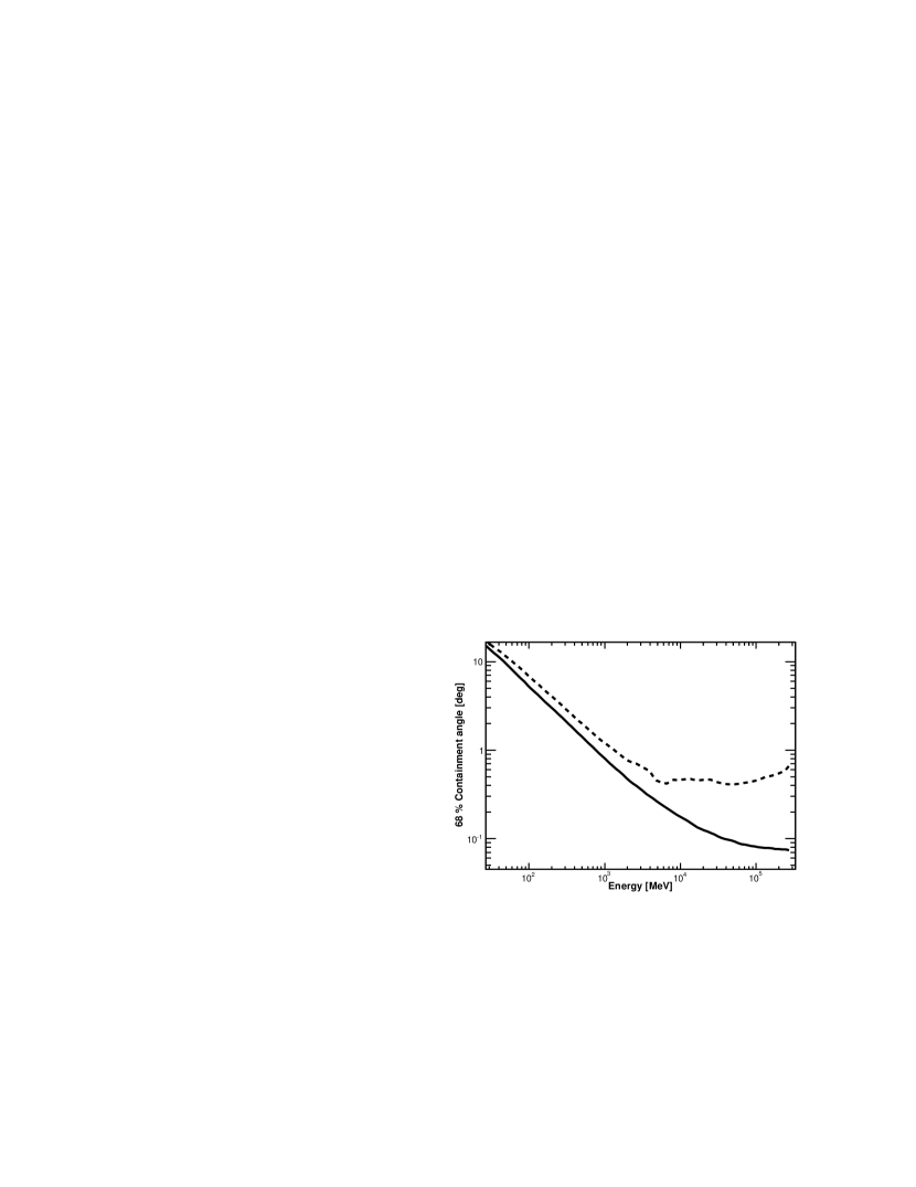
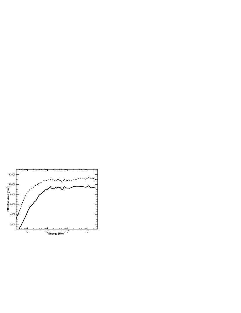
Figure 2: Left: Comparison of the estimated Point Spread Function (PSF) for the onboard and on-ground event reconstruction and selection. The black solid curve is the 68% containment angle on-axis for the transient event class, while the dashed curve represents the performance of the onboard reconstruction. Right: Comparison of the estimated onboard (dashed) and on-ground (solid black curve) on-axis effective areas. These estimates of the instrument response are based on simulations of the LAT.

The data telemetered to the ground consists of the signals from different parts of the LAT; from these signals the ground software must ‘reconstruct’ the events and filter out events that are unlikely to be gamma-rays. Therefore, the Instrument Response Functions (IRFs) depend not only on the hardware but also on the reconstruction and event selection software. For the same set of reconstructed events trade-offs in the event selection between retaining gamma rays and rejecting background result in different event classes. There are currently three standard event classes—the transient, source and diffuse event classes—that are appropriate for different scientific analyses (as their names suggest). Less severe cuts increase the photon signal (and hence the effective area) at the expense of an increase in the non-photon background and a degradation of the PSF and the energy resolution.

The least restrictive class, the transient event class, is designed for bright, transitory sources that are not background-limited. We expect that the on-ground event rate over the whole FOV above 100 MeV will be 2 Hz for the transient class and 0.4 Hz for the source class. In both cases we expect about one non-burst event per minute within the area of the PSF around the burst position. Consequently, there should be essentially no background during the prompt emission (with a typical duration of less than a minute) so that the transient class is the most appropriate—and in fact is the one used for producing all the results presented in this paper. On the other hand, the analysis of afterglows, which may linger for a few hours, will need to account for the non-burst background, at least in the low region of the energy spectrum, where the PSF is larger (see Fig. 2).

The onboard flight software also performs event reconstructions for the burst trigger. Because of the available computer resources, the onboard event selection is not as discriminating as the on-ground event selection, and therefore the onboard burst trigger is not as sensitive because the astrophysical photons are diluted by a larger background flux. Similarly, larger localization uncertainties result from the larger onboard PSF, as shown by the left-hand panel of Fig. 2.

3.3 $Fermi$ Gamma-ray Burst Monitor (GBM)

The GBM detects and localizes bursts, and extends $Fermi$’s burst spectral sensitivity to the energy range between 8 keV and 30 MeV or more. It consists of 12 NaI(Tl) (8–1000 keV) and 2 BGO (0.15–$>30$ MeV) crystals read by photomultipliers, arrayed with different orientations around the spacecraft. The GBM monitors more than 8 sr of the sky, including the LAT’s FOV, and localizes bursts with an accuracy of $<15\arcdeg$ (1$\sigma$) onboard, ($<3\arcdeg$ on ground), by comparing the rates in different detectors. The GBM is described in greater detail in Meegan et al. (2009, submitted).

3.4 $Fermi$’s Burst Operations

Both the GBM and the LAT have burst triggers. When either instrument triggers, a notice is sent to the ground through the TDRSS within $\sim 15$ s after the burst was detected and then disseminated by the Gamma-ray burst Coordinates Network (GCN) to observatories around the world. This initial notice is followed by messages with localizations calculated by the flight software of each detector. Additional data (e.g., burst and background rates) are also sent down by the GBM through TDRSS for an improved rapid localization on the ground by a dedicated processor.

Updated positions are calculated from the full datasets from each detector that are downlinked with a latency of a few hours. Scientists from both instrument teams analyze these data, and if warranted by the results, confer. Conclusions from these analyses are disseminated through GCN Circulars, free-format text that is e-mailed to scientists who have subscribed to this service. Both Notices and Circulars are posted on the GCN website.

If the observed burst fluxes in either detector exceed pre-set thresholds (which are higher for bursts detected by the GBM outside the LAT’s FOV), the FSW sends a request that the spacecraft slew to point the LAT at the burst location for a followup pointed observation; currently a 5 hr observation is planned.

In addition to the search for GRB onboard the LAT and manual follow-up analysis by duty scientists, there is also automated processing of the full science data. This processing performs an independent search for transient events in the LAT data, to greater sensitivity than is possible onboard, and also performs a counterpart search for all GRB detected within the LAT FoV. This is described in greater detail in § 6.3.

4 Burst Simulations

We test the $Fermi$ burst detection and analysis software with simulated data. These simulated data are based on our expectations for burst emission in the LAT and GBM spectral bands (see § 2), and on models of the instrument response of these two detectors. Since bursts undoubtedly differ from our theoretical expectations, our calculations are more reliable in showing the mission’s sensitivity to specific bursts than in estimating the number of bursts that will be detected.

We have two ‘GRB simulators’ that model the burst flux incident on each detector (Battelino et al., 2007a). The primary is the phenomenological simulator—described in greater detail below in § 4.1—that draws burst parameters from observed distributions. We have also created a physical simulator (Omodei, 2005; Omodei & Norris, 2007; Omodei et al., 2007) that calculates the synchrotron emission from the collision of shells in a relativistic outflow (the internal shock model—Piran 1999). For a given analysis we assemble an ensemble of simulated bursts using one of these GRB simulators. To simulate a LAT observation of each burst in this ensemble we create a realization of the photon flux, resulting in a list of simulated photons incident on the LAT. The LAT’s response to this photon flux is processed in one of two software paths. The first uses ‘GLEAM’, which performs a Monte Carlo simulation of the propagation of the photon and its resulting particle shower in the LAT (using the GEANT4 toolkit(Agostinelli et al., 2003)) and the detection of particles in the different LAT components(Atwood et al., 2004; Baldini et al., 2006). The photon is then ‘reconstructed’ from this simulated instrument response by the same software that processes real data. Thus GLEAM maps the incident photons into observed events. Our second, faster, processing pathway uses the instrument response functions to map the photons into events directly. We note that both approaches use the same input—a list of incident photons–and result in the same output—a list of ‘observed’ events in one of the event classes. In both approaches GRBs can be combined with other source types (such as stationary and flaring AGN, solar flares, supernova remnants, pulsars) to build a very complex model of the gamma-ray sky.

The GRB simulators also provide the input to the GBM simulation software. In this case the GRB simulators produce a time series of spectral parameters (usually the parameters for the ‘Band’ function—Band 2003—discussed above in § 2.1). The GBM simulation software samples the burst spectrum to create a list of incident photons and then uses a model of the GBM response to determine whether each photon is ‘detected,’ and if so, in which energy channel (simulating the GBM’s finite spectral resolution). Based on a model from the BATSE observations, background counts are added to the burst counts. The GBM simulation software outputs count lists, response matrices and background spectra in the standard FITS formats used by software such as XSPEC.

Because the GRB simulators provide input to both LAT and GBM simulations, simulated LAT and GBM data can be produced for the same bursts, allowing joint analyses. The $Fermi$ mission developed the ‘Standard Analysis Environment’ (SAE) to analyze both LAT and GBM data. Data can be binned in time, resulting in light curves (see, for example, Fig. 3), or in spectra that can be analyzed using a tool such as XSPEC. As will be described in § 7, joint fits of GBM and LAT data may cover an energy band larger than seven orders of magnitude (see Fig. 1). Consequently, $Fermi$ will be a very powerful tool for understanding the correlation between low-energy and high-energy GRB spectra.

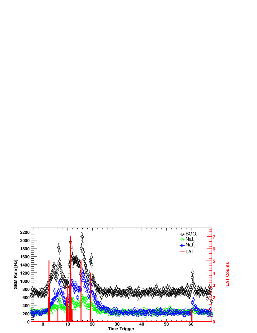
Figure 3: Simulated count rate light curve for a BGO detector, two NaI detectors, and the LAT for one simulated burst. In this model of the burst spectral evolution, the LAT detects counts at the beginning of each pulse; the correlation of the LAT and GBM light curves will be a powerful diagnostic of the emission processes. The simulation predicts that the LAT would detect a total of 42 gamma rays above 30 MeV in this moderately bright burst of 1 s peak flux of 63.37 ph cm^-2 s^-1 between 30 and 500 keV.

4.1 Phenomenological Burst Model

The phenomenological GRB simulator that is used for most of our simulations draws from observed spectral and temporal distributions to construct model gamma-ray bursts. This modeling assumes that bursts consist of a series of pulses that can be described by a universal family of functions (Norris et al., 1996)

$$I(t)=A\left\{\begin{array}[]{ll}\exp[-(|t-t_{0}|/\sigma_{r})^{\nu}],\hskip 28.45274ptt\leq t_{0}\\ \\ \exp[-(|t-t_{0}|/\sigma_{d})^{\nu}],\hskip 28.45274ptt>t_{0}\\ \end{array}\right.$$ (3)

where $\sigma_{r}$ and $\sigma_{d}$ parameterize the rise and decay timescale, and $\nu$ provides the ‘peakiness’ of the pulse. Although empirically $\sigma_{r}\sim 0.33~{}\sigma_{d}^{0.86}$, we approximate this relation as $\sigma_{r}\sim\sigma_{d}/3$. The pulse Full Width at Half Maximum (FWHM) is

$$W=(\sigma_{r}+\sigma_{d})\ln(2)^{1/\nu}.$$ (4)

Pulses are observed to narrow at higher energy in the BATSE energy band (Davis et al., 1994; Norris et al., 1996; Fenimore et al., 1995). Although the statistics in the EGRET data were insufficient to determine whether this narrowing continues in the $>$100 MeV band, our phenomenological model assumes that it does. We assume that the FWHM energy dependence is $W(E)\propto E^{-\xi}$ where $\xi$ is $\sim$0.4 (Fenimore et al., 1995; Norris et al., 1996). Thus, we give the pulse shape in eq. 3 an energy dependence by setting

$$\left\{\begin{array}[]{ll}\sigma_{d}(E)=0.75\times\ln(2)^{-1/\nu}W_{0}(E/20\hbox{ keV})^{-\xi}\\ \\ \sigma_{r}(E)=0.25\times\ln(2)^{-1/\nu}W_{0}(E/20\hbox{ keV})^{-\xi}.\end{array}\right.,$$ (5)

where $W_{0}$ is the FWHM at 20 keV. Burst spectra in the 10–1000 keV band are well-described by the ‘Band’ function (Band et al., 1993) parameterized in eq. 1. Empirically the Band function is an adequate description of burst spectra accumulated on short timescales (e.g., shorter than a pulse width) and over an entire burst. This may be due in part to the poor spectral resolution of scintillation detectors (such as BATSE and the GBM), but we will treat this as a physical characteristic of gamma-ray bursts. In the resulting model, the flux $f(t,E)$ is a product of a Band function with spectral indices $\alpha^{\prime}$ and $\beta^{\prime}$ and the energy-dependent pulse shape $I(t,E)$ (eq. 3 with eq. 5)

$$f(t,E)=I(t,E)~{}N_{\rm Band}(E|N_{0},E_{p},\alpha^{\prime},\beta^{\prime})\hskip 28.45274pt\hbox{ph cm${}^{-2}$ s${}^{-1}$ keV${}^{-1}$}.$$ (6)

Note that this spectrum is not strictly a Band function because the pulse shape function does not have a power law energy dependence.

The spectrum integrated over the entire burst is a Band function that is proportional to the product $W(E)N_{\rm Band}(E|N_{0},E_{p},\alpha^{\prime},\beta^{\prime})$. Because $W(E)$ is a power law with spectral index -$\xi$, the spectral indices $\alpha$ and $\beta$ for the integrated spectrum are different from the indices for the instantaneous flux (eq. 6)

$$\begin{array}[]{ll}\displaystyle\int_{-\infty}^{\infty}f(t,E)dt&=~{}N_{\rm Band}(E|N_{0},E_{p},\alpha,\beta)T=A_{0}~{}N_{\rm Band}(E|N_{0},E_{p},\alpha^{\prime},\beta^{\prime})~{}W(E)\\ &\\ &=~{}A_{0}~{}W_{0}~{}N_{\rm Band}(E|N_{0},E_{p},\alpha^{\prime}-\xi,\beta^{\prime}-\xi)\end{array}$$ (7)

where $T$ is the burst duration and all the normalizing factors resulting from the integration are incorporated in $A_{0}$. Thus the flux for a single GRB is the sum of many pulses of the form

$$f(t,E)=I(t,E)N_{\rm Band}(E|N_{0},E_{p},\alpha+\xi,\beta+\xi).$$ (8)

Drawn from observed burst distributions, the same spectral parameters $E_{p}$, $\alpha$ and $\beta$ are used for a given simulated burst. The number of pulses and parameters of each pulse (amplitude, width and peakedness) are also sampled from observed distributions (Norris et al., 1996).

Alternative spectral models have also been simulated; for example, Battelino et al. (2007a) describe simulations with a strong thermal photospheric component.

5 Semi-Analytical Sensitivity Estimates

The design of the LAT detector provides an ultimate burst sensitivity, regardless of whether the detection and analysis software achieves this ultimate limit. Thus in this section we estimate the LAT’s burst detection and localization capabilities, and the expected flux distribution. The following section describes the current burst detection algorithms.

5.1 Semi-Analytical Estimation of the Burst Detection Sensitivity

In this subsection we compute the LAT’s burst detection sensitivity using a semi-analytical approach based on the likelihood ratio test introduced by Neyman & Pearson (1928). This test is applied extensively to photon-counting experiments (Cash, 1979) and has been used to analyze the gamma-ray data from COS-B (Pollock et al., 1981, 1985) and EGRET (Mattox et al., 1996). The statistic for this test is the likelihood for the null hypothesis for the data divided by the likelihood for the alternative hypothesis, here that burst flux is present. This methodology is the basis of the likelihood tool that will be used to analyze LAT observations; here we perform a semi-analytic calculation for the simple case of a point source on a uniform background.

In photon-counting experiments, the natural logarithm of the likelihood for a given model can be written as

$$\ln(L)=\sum_{photons}\ln(M_{i})-N_{\mathrm{pred}}+\mathrm{constant}$$ (9)

where $M_{i}$ is the predicted photon density at the position and time of $i$th observed count, and $N_{\mathrm{pred}}$ is the predicted total number of counts. We compare the log likelihood for the null hypothesis that only background counts are present versus the hypothesis that both burst and background counts are present.

The expected number of counts from a burst flux $S(E)$ is

$$N_{S}=T_{obs}\int_{\Delta\Omega}\int_{E_{1}}^{E_{2}}A_{eff}(E)S(E)F(E,\Omega)\,dEd\Omega$$ (10)

while the expected number of counts from a background flux $B(E)$ (assumed to be uniformly distributed over the sky) is

$$N_{B}=T_{obs}\int_{E_{1}}^{E_{2}}A_{eff}(E)B(E)dE\Delta\Omega$$ (11)

where $A_{eff}$ is the effective area and $F(E,\Omega)$ is the normalized PSF (which therefore does not show up in eq. 11). Note that $B(E)$ varies significantly over the sky, but our assumption is that it is constant over $\Delta\Omega$.

The logarithm of the likelihood of the null hypothesis is

$$\ln(L_{0})=T_{obs}\int_{\Delta\Omega}\int_{E_{1}}^{E_{2}}A_{eff}(E)\left[S(E)F(E,\Omega)+B(E)\right]\times$$

$$\ln(A_{eff}(E)B(E))dEd\Omega-N_{B}\quad.$$ (12)

The actual count rate is assumed to result from both background and burst flux while the predicted count rates (the $M_{i}$ in eq. 9 and the total number of counts $N_{\rm pred}$) are calculated only for the background flux (the null hypothesis).

Similarly, the logarithm of the likelihood of the hypothesis that a burst is present is

$$\ln(L_{1})=\left[T_{obs}\int_{\Delta\Omega}\int_{E_{1}}^{E_{2}}A_{eff}(E)\left[S(E)F(E,\Omega)+B(E)\right]\right.\times$$

$$\left.\ln\left(A_{eff}(E)\left[S(E)F(E,\Omega)+B(E)\right]\right)dEd\Omega\right]-(N_{S}+N_{B})\quad.$$ (13)

Here both the actual and predicted count rates are calculated for both burst and background fluxes.

Wilks’ theorem (Wilks, 1938) defines the Test Statistic as $T_{S}=-2(\ln(L_{0})-\ln(L_{1}))$, and states that $T_{S}$ is distributed (asymptotically) as a $\chi^{2}$ distribution of $m$ degrees of freedom, where $m$ is the number of burst parameters. From eqs. 12 and 13 $T_{S}$ is

$$T_{S}=2~{}T_{obs}\int_{\Delta\Omega}\int_{E_{1}}^{E_{2}}A_{eff}(E)B(E)\left[\left(1+G(E,\Omega)\right)\ln\left(1+G(E,\Omega)\right)-G(E,\Omega)\right]dEd\Omega$$ (14)

where we have defined a signal-to-noise ratio $G(E,\Omega)=S(E)F(E,\Omega)/B(E)$.

The significance of a source detection in standard deviation units is calculated as $N_{\sigma}=\sqrt{T_{S}}$ in the case $m=1$ ($\chi^{2}$ with 1 dof). Here we assume that Wilks’ theorem holds, which might be not absolutely true in a low-count regime (see, in particular, the discussion in § 6.5). However, we will see that this method gives a robust estimate of the LAT sensitivity to GRBs. We can use this method to estimate the LAT sensitivity to GRB.

In our modeling we assume the burst has a ‘Band’ function spectrum (see eq. 1) and that the flux is constant over a duration $T_{GRB}$. Since we seek the optimal detection sensitivity, we calculate $T_{S}$ for $T_{obs}=T_{GRB}$. We assume a spatially uniform background with a power law spectrum

$$B(E)=B_{0}\left(\frac{E}{\hbox{100 MeV}}\right)^{\gamma}\quad\hbox{ph cm${}^{-2}$ MeV${}^{-1}$ s${}^{-1}$ sr${}^{-1}$}$$ (15)

where the value of the normalization constant $B_{0}$ is set to mimic the expected background rate. For modeling the onboard trigger the background rate above 100 MeV is set to 120 Hz, while, for the on-ground trigger the background is set to 2 Hz, as will be discussed below. The spectral index is set to be $\gamma=-2.1$. The results depend on the value of the spectral index; a detailed study of the dependence of the results as a function of the shape of the residual background is outside the illustrative goal of this section, thus we omit such discussion. We require $T_{S}\geq 25$ and at least 10 source counts in the LAT detector, corresponding to a threshold significance of 5$\sigma$ and a minimum number of GRB counts to see a clear excess in the LAT data even in the case of very few background events. We use the “transient” event class described in § 3.2, and compute the minimum 50–300 keV fluence of bursts at this detection threshold. The burst fluxes in the LAT band depend only on the high energy power law component of the ‘Band’ spectrum; assumed values of the low energy power law spectral index $\alpha=-1$ and $E_{p}=500$ keV are used to express the spectrum’s normalization in familiar fluence units. Results are shown in Fig. 4; at short durations the threshold is determined by the finite number of burst photons, while the background determines the threshold for longer durations. This figure predicts that unless other high-energy spectral components are present, the bursts detected by the LAT will be ‘hard’ with photon indices $\beta$ near $-2$ (Band, 2007).

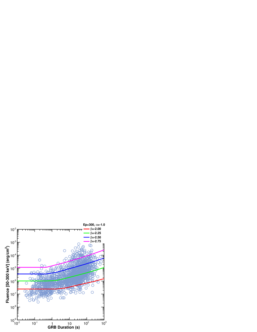
Figure 4: Threshold fluence as a function of the GRB duration, for on-ground detection and for on-axis incidence. Threshold fluence increases by factor of $\sim$ 2 for z-axis angles of 50 degrees. Different lines are related to different spectral index. Also plotted are the observed bursts from the BATSE catalog.

These estimates consider the detectability of individual bursts. We can compute the sensitivity of the LAT detector to GRB considering as input the observed distribution of GRB with known spectral parameters. We use the catalog of bright bursts (Kaneko et al., 2006) to quantify the characteristics of GRBs. This catalog contains 350 bright GRBs over the entire life of the BATSE experiment selected for their energy fluence (requiring that the fluence in the 20-2000 keV band is greater than 2$\times$10^-5 erg/cm²) or on their peak photon flux (over 256 ms, in the 50-300 keV, greater than 10 ph/cm²/s). This subset of burst of the whole BATSE catalog represents the most comprehensive study of spectral properties of GRB prompt emission to date and is available electronically from the High-Energy Astrophysics Science Archive Research Center (HEASARC). We restrict our sample of GRB to the ones with a well reconstructed $E_{peak}$; furthermore, we exclude the bursts described by the Comptonized model (COMP) for which an emission at LAT energy is very unlikely; we also reject bursts with spectra described by a single power law with undetermined $E_{peak}$ (probably outside the BATSE energy range).

Considering the field of view of the BATSE experiment and these selection criteria, we estimate a rate of 50 GRB per year (full sky). For each burst we simulate, the duration, the energy fluence and the spectral parameters are in agreement with one of the bursts in the Bright BATSE catalog. Its direction is randomly chosen in the sky, and for each burst we compute the LAT response functions for that particular direction. Finally, we compute $T_{s}$ using eq. 14. The resulting distributions are given by Fig. 5.

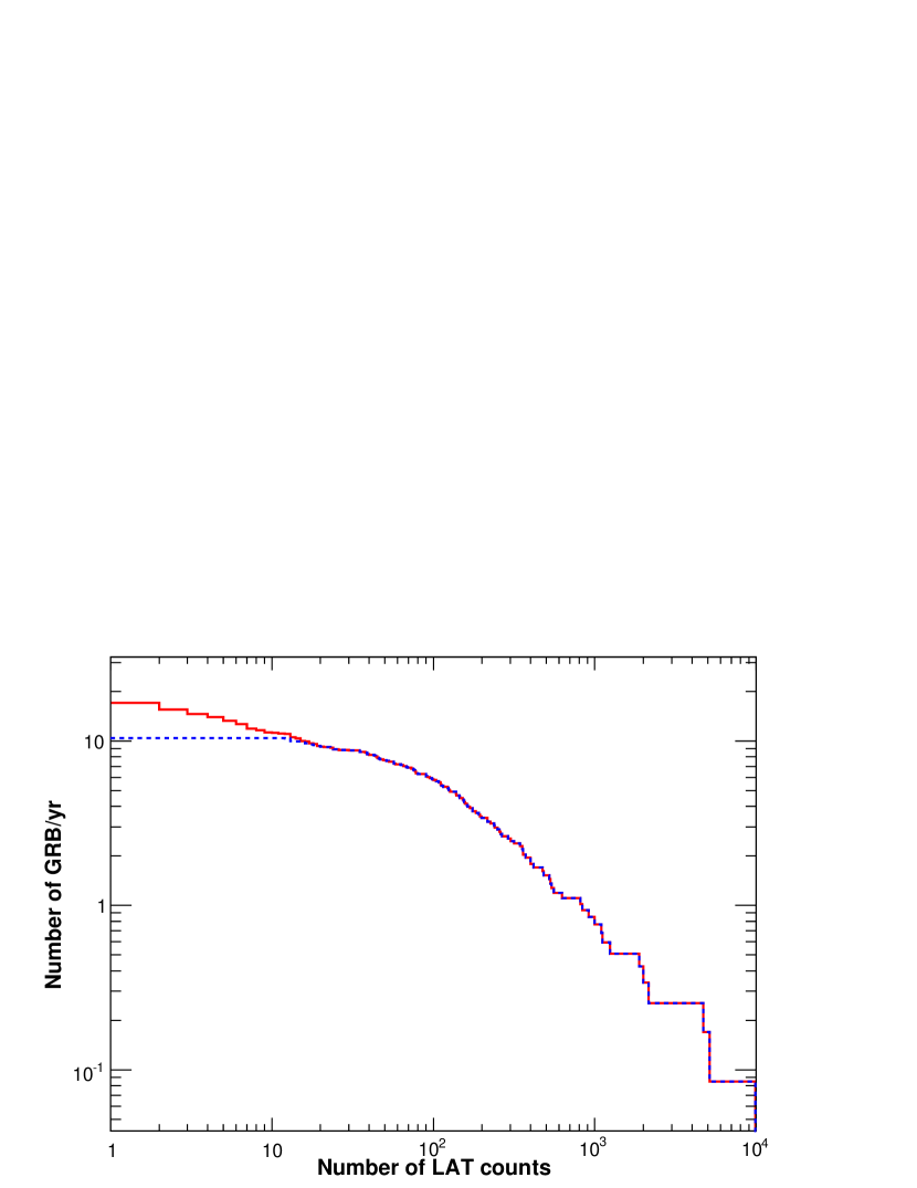
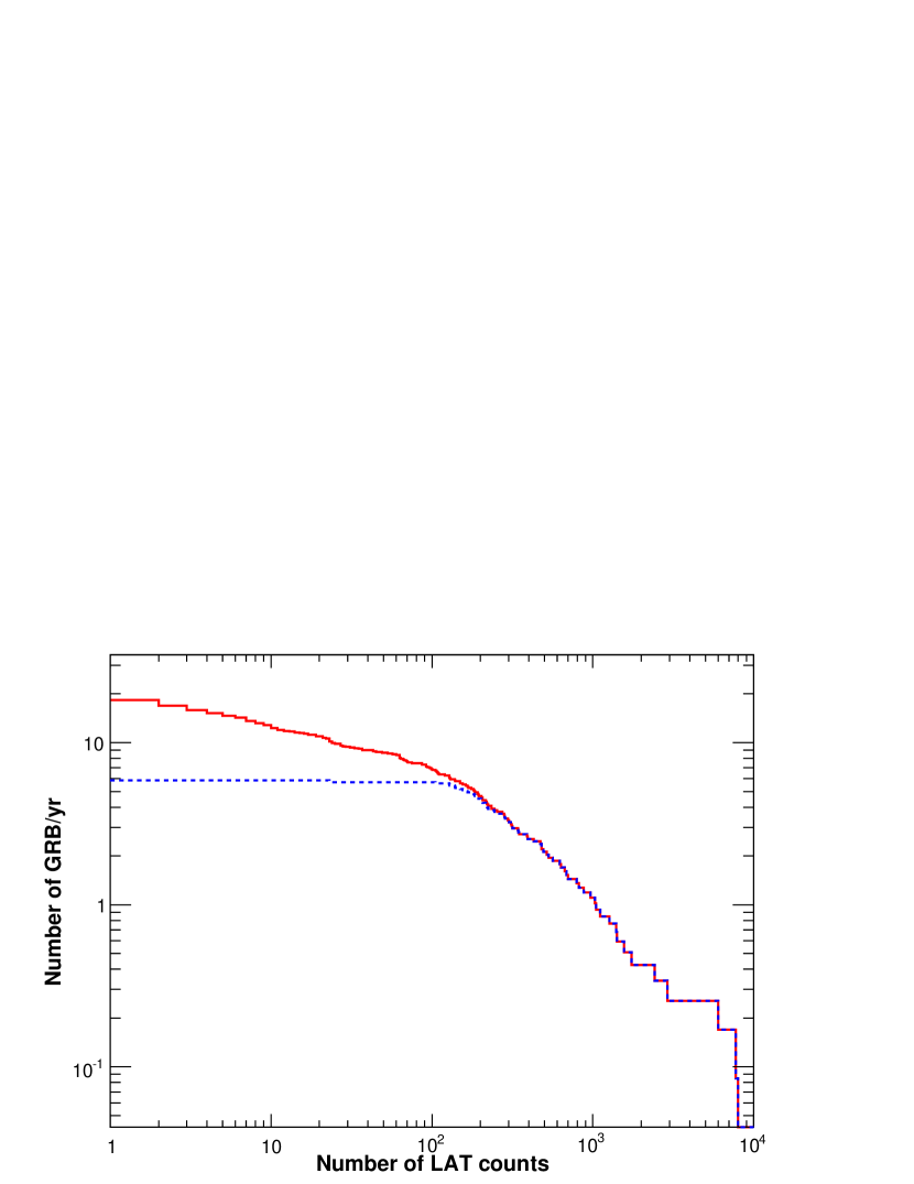
Figure 5: Integrated number of GRBs per year as a function of the number of LAT counts. The solid curve shows all bursts in the sample, while the dashed curve gives the detected bursts. Left panel: on-ground analysis (“transient” class, 2 Hz background rate above 100 MeV). Right panel: onboard analysis (120 Hz background rate).

The onboard analysis’ larger effective area (Fig. 2) results in a larger cumulative burst rate, but not a larger detected rate because of the larger background rate. Events that are processed onboard by the GRB search algorithm are downloaded, and a looser set of cuts can be chosen on-ground in order to optimize the signal/noise ratio. We emphasize that this calculation makes a number of simplifying assumptions. The LAT spectrum is assumed to be a simple extrapolation of the spectrum observed by BATSE. Spectral evolution within a burst is not considered. The BATSE burst population was biased by that instrument’s detection characteristics. Nonetheless we estimate that the LAT can detect around 1 burst per month, with a few bursts per year having more than 100 counts. These few bright bursts are likely to have a large impact on burst science since detailed spectral analysis will be possible.

In the framework described in this section, we can also estimate the localization accuracy for the burst sample, for both onboard and on-ground triggers. If $\sigma_{i}$ is the 68$\%$ containment radius for the single photon PSF, then the localization is computed as

$$\sigma_{GRB}^{-1}=\sqrt{\sum_{i}{\frac{1}{\sigma_{i}^{2}}}}$$ (16)

that, in terms of the previously defined quantities, is

$$\sigma_{GRB}^{-1}=\sqrt{\frac{T_{GRB}}{3}\int_{E_{1}}^{E_{2}}\frac{A_{eff}(E)S(E)}{\sigma_{68\%}(E)^{2}}dE}$$ (17)

The factor of 3 takes into account the non-gaussianity of the PSF, and was estimated by Burnett (2007). We compute the localization accuracy for each burst in our sample. Fig. 6 shows the results. In each plot the detected burst are represented by red triangles, while the blue empty circles are the bursts with LAT counts that did not pass our detection condition.

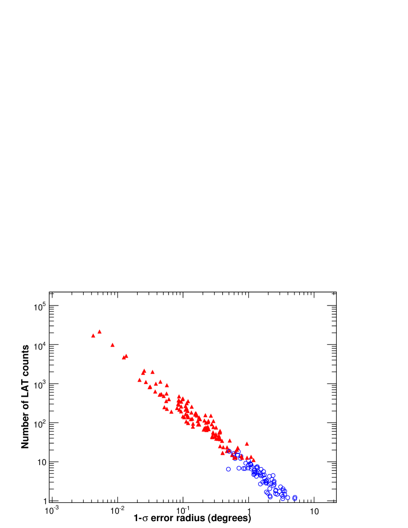
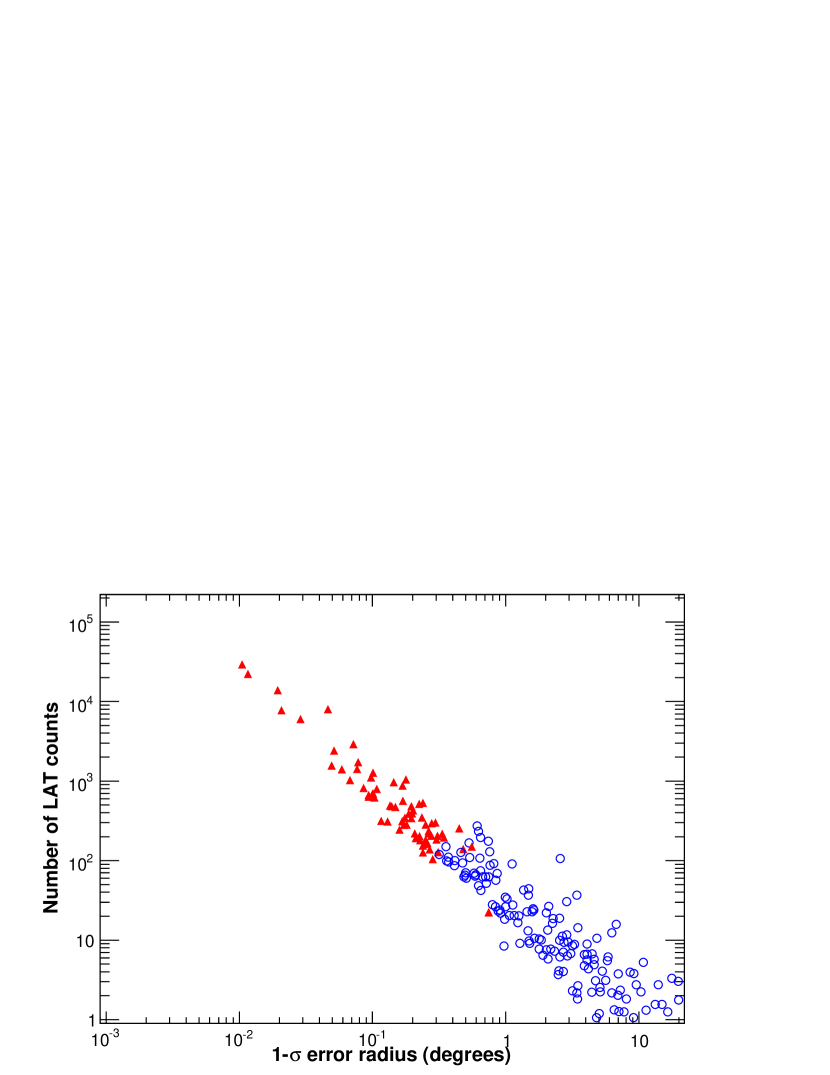
Figure 6: Number of LAT counts vs. localization accuracy. In each panel the red triangles denote detected bursts and the open blue circles show undetected bursts. The left and right panels are for the on-ground and onboard localizations. Thus the on-ground analysis results in a slightly larger burst detection rate and a better localizations. The superior track reconstruction and background reduction outweighs the smaller effective area in increasing the on-ground detection rate.

These results show that the LAT can localize bursts with sub-degree accuracy, both onboard and on-ground. The GRB yield is greater and bursts are better-localized on-ground than onboard. The on-ground analysis is available only after the full dataset is downlinked and processed. This process can lasts few hours, depending on the position of the downlink contact. Onboard localization is delivered quasi-real time with onboard alerts. For those bursts, multiwavelength follow-ups will be feasible for bursts localized within a few tens of arcminutes. For example, the FOV of Swift’s XRT is about 0.4^∘ and is of the same order as the FOV of the typical mid-size optical or near-IR (NIR) telescope. Afterglow searches in the optical and NIR are very successful—$\sim$60% of the Swift bursts have been associated with optical and NIR afterglows. Fig. 6 shows that a sizeable fraction of $Fermi$ GRB detections will be localized within these requirements, and relatively large FOV ground-based observatories ($\sim$30 arcmin) with optical/NIR filters (I, z, J, H, K) should produce a fairly high detection rate for the afterglows of LAT-detected GRBs.

5.2 Estimated LAT Flux Distribution

We now consider the full GRB model described in § 4 for estimating the expected LAT flux distribution. This is, of course, very dependent on the assumptions of the GRB model, and the final result should be considered only as a prediction of the flux distribution.

We use the bright BATSE catalog (Kaneko et al., 2006) for the burst population, as described in the previous section. In addition, we also select a sub-sample of bursts for which beta is more negative than -2. This is motivated by the fact that a power law index greater than -2 implies a divergence in the released content of energy, thus those value are unphysical and a cut-off should take place. The measurements yielding beta greater than -2 are questionable and suggest either an ill-determined quantity for a true spectrum that is in reality softer, or an additional spectral break above the energies measured with BATSE. Given the duration, the number of pulses is fixed by the total burst duration. Pulses are combined together in order to obtain a final $T_{90}$ duration. Correlations between duration, intensity, and spectral parameters are automatically taken into account as each of these bursts corresponds to an entry in the Kaneko et al. catalog. The emission is extended up to high energy with the model described in § 4.

We emphasize again that this model ignores possible intrinsic cutoffs (resulting from the high end of the particle distribution or internal opacity—§ 2.2.2), and additional high-energy components suggested by the EGRET observations (§ 2.1). High-energy emission ($>$10 GeV) is also sensitive to cosmological attenuation due to pair production between the GRB radiation and the Extragalactic Background Light (EBL—§ 2.2.2). The uncertain EBL spectral energy distribution resulting from the absence of high redshift data provides a variety of theoretical models for such diffuse radiation. Thus the observation of the high-energy cut-off as a function of the GRB distance can, in principle, constrain the background light. In our simulation we include this effect, adopting the EBL model in Kneiske et al. (2004). Short bursts are thought to be the result of the merging of compact objects in binary systems, so we adopt the short burst redshift distribution from Guetta & Piran (2005), while long bursts are related to the explosive end of massive stars, whose distributions are well traced by the Star Formation History (Porciani & Madau, 2001).

In Fig. 7 the sampled distributions are shown. The Dashed line histogram is obtained from the full bright burst BATSE catalog. In order to increase the number of burst in the field of view of the LAT detector we over-sampled the original catalog by a factor 1.4. The dark filled histograms show the distribution of GRB with at least 1 count in the LAT detector, and the light filled histograms are the sub-sample of detected GRB with beta $<$ -2.

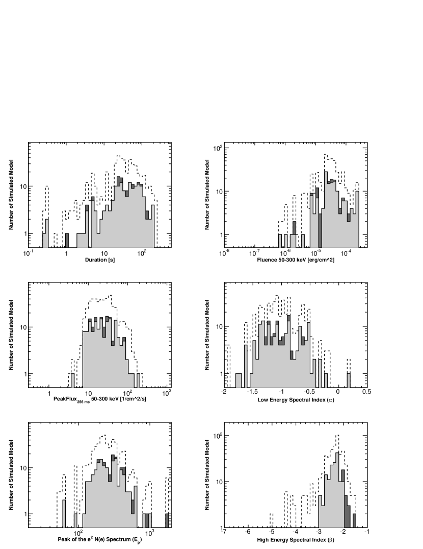
Figure 7: Parameter distributions for the simulated bursts of the bright burst BATSE catalog (dashed lines). Filled dark histograms represent the GRBs with more than 1 predicted count above 100 MeV in the LAT detector, while for the light filled histograms we have also required that the high-energy spectral index beta is more negative than -2. The distributions show the logarithm of the duration, the fluence, the peak flux distribution, the low and high energy spectral indexes and the logarithm of the energy of the peak of the $\nu F_{\nu}$ spectrum.

We simulate approximately ten years of observations in scanning mode. The orbit of the $Fermi$ satellite, the South Atlantic Anomaly (SAA) passages and Earth occultations are all considered. In Fig. 8 we plot the number of expected bursts per year as a function of the number of photons per burst detected by the LAT. The different couples of lines refer to different energy thresholds (100 MeV, 1 GeV, and 10 GeV). Dashed lines are the same computation but using only the sub-sample of GRBs with beta more negative than -2 (the light filled distribution in Fig. 7). The EBL attenuation affects only the high-energy curve, as expected from the theory, leaving the sensitivities almost unchanged below 10 GeV. Assuming that the emission component observed in the 10–1000 MeV band continues unbroken into the LAT energy band, we estimate that the LAT will independently detect approximately 10 bursts per year, depending on the sensitivity of the detection algorithm; approximately one burst every three months will have more than a hundred counts in the LAT detector above 100 MeV: these are the bursts for which a detailed spectral or even time resolved spectral analysis will be possible. If we restrict our analysis to the sub-sample of bursts with beta more negative than -2, these numbers decrease. Nevertheless, even if we adopt this conservative approach, LAT should be able to detect independently approximately 1 burst every two months, and will be able to detect radiation up to tens of GeV.

With the assumed high-energy emission model a few bursts per year will show high-energy prompt emission, with photons above 10 GeV. These rates are in agreement with the number of bursts detected in the LAT data after few months (GRB080825C (Bouvier et al., 2008), GRB080916C (Tajima et al., 2008), GRB081024B (Omodei, 2008)), but the statistics is still low for any strong constraint on the burst population.

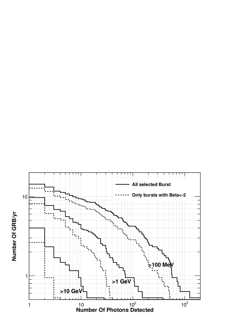
Figure 8: Model-dependent LAT GRB sensitivity. The GRB spectrum is extrapolated from BATSE to LAT energies. The all-sky burst rate is assumed to be 50 GRB yr^-1 full sky (above the peak flux in 256 ms of 10 ph s^-1 cm^-2 in the 50-300 keV or with an energy flux in the 20-2000 keV band greater than 2$\times$ 10^-5 erg/cm²), based on BATSE catalog of bright bursts. The effect of the EBL absorption is included. Different curves refer to different energy thresholds. Dashed curves are the result of the analysis excluding very hard bursts, with a beta greater than -2.

6 Gamma-Ray Burst Detection

The rapid detection and localization of bursts is a major goal of the $Fermi$ mission. Both $Fermi$ instruments will search for bursts both onboard and on-ground. These searches will detect bursts on different timescales and with different sensitivities. Here we focus on LAT burst detection, but for completeness we describe briefly GBM burst detection.

6.1 GBM Burst Detection

Onboard the $Fermi$ observatory the GBM will use rate triggers that monitor the count rate from each detector for a statistically significant increase. Similar to the BATSE detectors, the GBM as a whole will trigger when two or more detectors trigger. A rate trigger compares the number of counts in an energy band $\Delta E$ over a time bin $\Delta t$ to the expected number of background counts in this $\Delta E$–$\Delta t$ bin; the background is estimated from the rate before the time bin being tested. The GBM trigger uses the twelve NaI detectors with various energy bands, including $\Delta E$=50–300 keV, and time bins from 16 ms to 16.384 s. Note that the BATSE trigger had one energy band—usually $\Delta E$=50–300 keV—and the three time bins $\Delta t=$0.064, 0.256, and 1.024 s. The GBM burst detection algorithms are described in greater detail in Meegan et al. (2009, submitted).

When the GBM triggers it sends a series of burst alert packets through the spacecraft and TDRSS to the Earth. Some of these burst packets, including the burst location calculated onboard, will also be sent to the LAT to assist in the LAT’s onboard burst detection. Burst locations are calculated by comparing the rates in the different detectors; each the detectors’ effective area varies across the FOV. In addition, the GBM will send a signal over a dedicated cable to the LAT; this signal will only inform the LAT that the GBM has triggered.

The continuous GBM data that are routinely telemetered to the ground can also be searched for bursts that did not trigger the GBM onboard. These data will provide rates for all the GBM detectors in 8 energy channels with 0.256 s resolution and in 128 energy channels with 4.096 s resolution. In particular, if a burst triggers the LAT but not the GBM, these rates will at the very least provide upper limits on the burst flux in the GBM energy band.

6.2 Onboard LAT Detection

The LAT flight software will detect bursts, localize them, and report their positions to the ground through the burst alert telemetry. The rapid notification of ground-based telescopes through GCN will result in multi-wavelength afterglow observations of GRBs with known high energy emission. The onboard burst trigger is described in Kuehn et al. (2007).

The onboard processing that results in the detection of a GRB can be subdivided into three steps: initial event filtering; event track reconstruction; and finally burst detection and localization. In the first step all events—photons and charged particles—that trigger the LAT hardware are filtered to remove events that are of no further scientific interest. The events that survive this first filtering constitute the science data stream that is downlinked to the ground for further processing. These events are also fed into the second step of the onboard burst processing pathway.

The second step of the burst pathway attempts to reconstruct tracks for all the events in the science data stream using the ‘hits’ in the tracker’s silicon strip detectors that indicate the passage of a charged particle. The burst trigger algorithm uses both spatial and temporal information, and therefore a 3-dimensional track that points back to a photon’s origin is required. Tracks can be calculated for only about a third the events that are input to this step, although surprisingly the onboard track-finding efficiency is 80% to 90% of the more sophisticated ground calculation. However, the onboard reconstruction is less accurate, resulting in a larger PSF onboard than on-ground, as is shown by Fig. 2. A larger fraction of the incident photons survive the onboard filtering than survive the on-ground processing at the expense of a much higher non-photon background onboard than on-ground; consequently the onboard effective area is actually larger than the on-ground effective area, as Fig. 2 shows.

The rate of events that pass the onboard gamma filter (currently the same event set that is downlinked and thus available on-ground) is $\sim$400 Hz. The rate that events are sent to the onboard burst trigger, which requires 3-dimensional tracks, is $\sim$120 Hz. The on-ground processing creates a transient event class with a rate of $\sim$2 Hz. Thus onboard the burst trigger must find a burst signal against a background of $\sim$120 non-burst events, while on-ground this background is only $\sim$2 Hz. This difference in non-burst background rate sets fundamental limits on the onboard and on ground burst detection sensitivities.

The third step in the burst processing is burst detection, which considers the events that have passed all the filters of the first two steps, and thus have arrival times, energies and origins on the sky. When a detector such as the GBM provides only event rates, the burst trigger can only be based on a statistically significant increase in these rates. However, when a detector such as the LAT provides both spatial and temporal information for each event, then an efficient burst trigger will search for temporal and spatial event clustering. Most searches for transients bin the events in time and space (if relevant), but the LAT uses an unbinned method.

The LAT burst trigger searches for statistically significant clusters in time and space. The trigger has two tiers. The first tier identifies potentially interesting event clusters for further investigation by the second tier; the threshold for the first tier allows many false tier 1 triggers that are then rejected by the second tier. The first tier operates continuously, except while the second tier code is running. A GBM trigger is equivalent to a first tier trigger in that the GBM’s trigger time and position are passed directly to the second tier.

Tier 1 operates on sets of $N$ events that survived the first two steps, where currently $N$ is in the range of 40–200. The effective time window that is searched is $N$ divided by the event rate; for an event rate of 120 Hz and these values of $N$, the time window is 1/3–5/3 s. Each of these $N$ events is considered as the seed for a cluster consisting of all events that are within $\theta_{0}$ of the seed; currently $\theta_{0}=17^{\circ}$, approximately the 68% containment radius of the onboard 3D tracks at low event energies. A clustering statistic, described below, is then calculated for each cluster. A tier 1 trigger results when a clustering statistic for any cluster exceeds a threshold value. A candidate burst location is then calculated from the events of the cluster that resulted in the tier 1 trigger.

The onboard burst localization algorithm uses a weighted average of the positions of the cluster’s events. The weighting is the inverse of the angular distance of an event from the burst position. Since the purpose of the algorithm is to find the burst position, the averaging must be iterated, with the weighting used in one step calculated from the position from the previous step. The initial location is the unweighted average of the events positions. The convergence criterion is a change of 1 arcmin between iterations (with a maximum of 10 iterations). The position uncertainty depends on the number and energies of events, but the goal is an uncertainty less that 1^∘. Using Monte Carlo simulations, this methodology was found to be superior to others that were tried.

The tier 1 trigger time and localization (or if the GBM triggered, its trigger time and burst position) are then passed to the second tier. Because the second tier is run relatively infrequently, it can consider a much larger set of events than the first tier. Currently 500 events are considered, which corresponds to a time window of $\sim$4.2 s. A cluster is then formed from all events in this set that are within $\theta_{2}$ ($\sim 10^{\circ}$) of the tier 1 burst location. A clustering statistic is then calculated for this cluster, and if its value exceeds a threshold, a tier 2 trigger results and the cluster events are run through the localization algorithm. The resulting trigger time, burst location and number of counts in four energy bands are then sent to the ground through the burst alert telemetry. The second tier is run repeatedly after a tier 1 trigger in case the burst brightens resulting in a larger cluster centered on the tier 1 position, and consequently a tier 2 trigger (if one has not yet occurred) and a better burst localization (if a tier 2 trigger does occur).

The clustering statistic is based on the probabilities that the cluster’s events have the observed distances from the cluster seed position and the arrival time separations, under the null hypothesis that a burst is not occurring. Assuming events are thrown uniformly onto a sphere (the null hypothesis), the probability $p_{s}$ of finding an event within $\theta$ degrees of the cluster seed position is

$$p_{s}=\frac{1-\mathrm{cos}(\theta)}{1-\mathrm{cos}(\theta_{m})}$$ (18)

where it is assumed that there are no events at more than $\theta_{m}=115^{\circ}$ (the performance is not sensitive to this parameter). Thus for a cluster of $M$ events the spatial contribution to the clustering statistic is

$$P_{S}=\sum_{i=1}^{M}\,|\mathrm{log}_{10}(p_{s_{i}})|=\sum_{i=1}^{M}\Bigg{|}\mathrm{log}_{10}\bigg{(}\,\frac{1-\mathrm{cos}(\theta_{i})}{1-\mathrm{cos}(\theta_{m})}\bigg{)}\Bigg{|}\;.$$ (19)

The temporal part of the cluster probability assumes that the event arrival time follows a Poisson distribution (again the null hypothesis). The probability that the arrival times of two subsequent events differ by $\Delta T$ is

$$p_{t}=1-\exp[-r_{t}\Delta T]\quad,$$ (20)

where $r_{t}$ is the rate at which events occur within the area of the cluster. The temporal contribution of each cluster to the clustering statistic is

$$P_{T}=\sum_{i=1}^{M}|\mathrm{log}_{10}(p_{t_{i}})|=\sum_{i=1}^{M}\bigg{|}\mathrm{log}_{10}(1-e^{-r_{t}\Delta T_{i}})\,\bigg{|}\;.$$ (21)

The trigger criterion is

$$\xi P_{T}+P_{S}>\Theta$$ (22)

where $\xi$ is an adjustable parameter that assigns relative weights to the spatial and temporal clustering, and $\Theta$ is the threshold. The two tiers may use different values of both $\xi$ and $\Theta$. The overall false trigger rate depends on the tier 2 value of $\Theta$.

The parameters used by the onboard burst detection and localization software are sensitive to the actual event rates, and will ultimately be set based on flight experience. Currently the thresholds are set high enough to preclude any triggers, and diagnostic data is being downlinked and studied. The thresholds will eventually be lowered, keeping the false trigger rate at an acceptable level.

Based on preliminary calculations using a burst population based on BATSE, we estimate $\sim$1 bursts every two months will be detected and localized to $1^{\circ}$ (see Fig. 5 and Fig. 6).

6.3 LAT Ground-Based Blind Search

A burst detection algorithm will be applied on the ground to all LAT counts after the events are reconstructed and classified to detect bursts that were not detected by the onboard algorithm, the GBM, or other missions and telescopes. Thus this ‘blind search’ is similar to the first tier of the onboard burst detection algorithm. The ground-based search will be performed after each satellite downlink; to capture bursts that straddle the downlink boundaries, some counts from the previous downlink are buffered and used in searching for bursts in the data from a given downlink. The ground-based blind search algorithm is very similar to the onboard algorithm described in the previous section, but will benefit from the full ground-based event reconstruction and background rejection techniques that are applied to produce the LAT counts used for astrophysical analysis. For these data, the particle background rates will be lower than the onboard rates by at least two orders-of-magnitude. Furthermore, the reconstructed photon directions and energies will be more accurate than the onboard quantities. Fig. 2 compares the 68% containment angle as a function of the photon energy for the onboard and on-ground LAT count datasets.

In addition to differing in the reconstruction and background filtering, the ground-based analysis treats the input data slightly differently. The first stage of the ground-based algorithm is applied to consecutive sets of 20 to 100 counts. As with the onboard algorithm, the number of counts analyzed is configurable and will be adjusted with the growth of our knowledge of GRB prompt emission in the LAT band and of the residual instrumental background. However, in contrast to the onboard algorithm, the data sets do not overlap. This ensures that each segment is statistically independent and generally better separates the log-probability distributions of the null case (i.e., where there is no burst) from the distributions computed when burst photons are present. Fig. 9 shows the reference distribution for the null case derived from simulated background data. We modeled the low end (large negative values) of the distribution with a Gaussian, and set the burst detection threshold at 5$\sigma$ from the fitted peak. Since this distribution is derived from pre-launch Monte Carlo simulations with assumed incident particle distributions and other expected on-orbit conditions, the thresholds are being re-calibrated with real flight data. Since we perform an empirical threshold calibration, we can neglect the constant normalization factors in the denominators of the single event probabilities shown in eqs. 18 and  20.

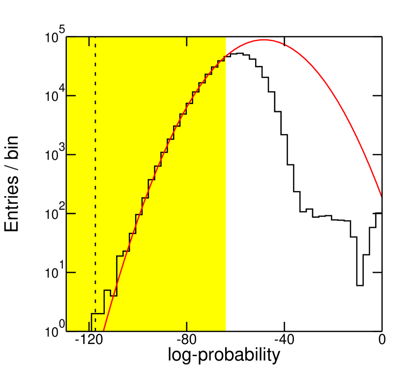
Figure 9: Distribution of log-probability values under the null hypothesis obtained from applying the ground-based version of the GRB search algorithm to sets of 20 counts. The shaded region indicates the range over which a Gaussian function, shown in red, was fit to these data. The resulting 5$\sigma$ threshold at an overall log-probability value of $-117$ is plotted as the vertical dashed line. Burst candidates are required to have log-probabilities below this threshold.

The overall log-probability is the sum of spatial and temporal components (see eq. 22), which we weight equally ($\xi$=1). Fig. 10 shows the 2D distributions for the temporal and spatial components. The dashed line in Fig. 10 corresponds to the 5$\sigma$ threshold with this weighting. Fig. 11 shows the time history of the log-probabilities as applied to the GRB grid data. The excursions across the threshold line indicate the burst candidates.

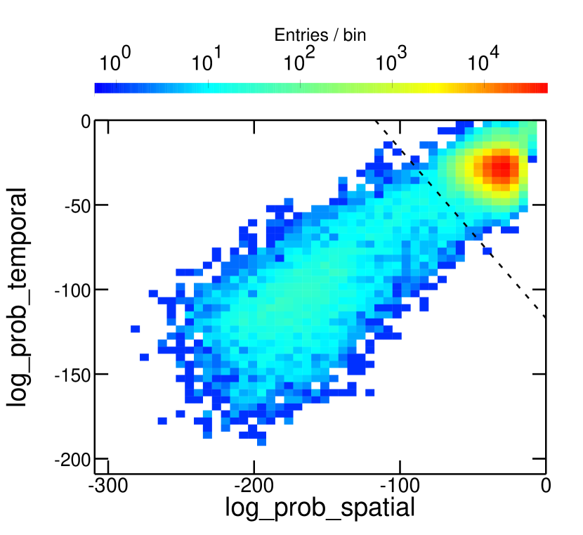
Figure 10: 2D histogram of the spatial and temporal log-probability components. The dashed line indicates the 5$-\sigma$ threshold (an overall log-probability value of $-117$) derived from the null distribution (figure 9). Burst candidates are required to lie below this line.

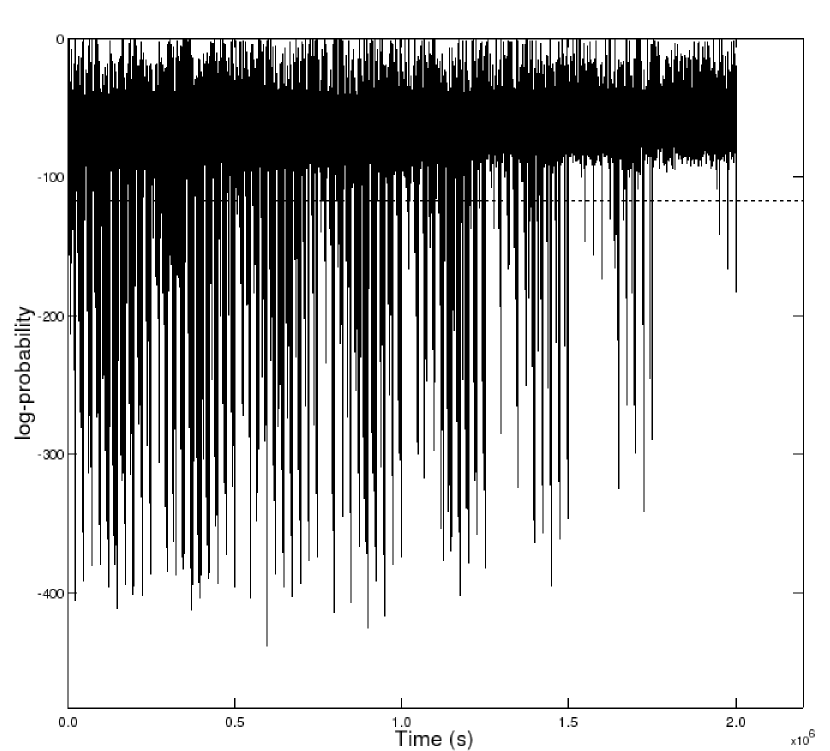
Figure 11: Time history of the ground-based log-probability. The horizontal dashed line shows the 5$\sigma$ threshold derived from the Gaussian function fit to the log-probabilities distribution under the null hypothesis (Fig. 9). Burst candidates are required to lie below this line.

While the onboard burst trigger performs two passes through the data with the temporal-spatial clustering likelihood algorithm, the ground-based detection analysis performs only one such pass. If a candidate burst is found in the ground-based analysis, counts from a time range bracketing the trigger time undergoes further processing to determine the significance of the burst. If the burst is sufficiently significant, it is localized and its spectrum is analyzed. These analyses use the unbinned maximum likelihood method that is applied to LAT point sources.

6.4 GRB Candidate Follow-up Processing

When a candidate burst location and trigger time is provided by the ground-based blind search, a LAT or GBM onboard trigger, or another burst detector such as Swift—we will call this a first stage detection—a LAT ISOC data processing pipeline will analyze the LAT counts to determine the significance of a possible LAT detection. This step in deciding whether the LAT has detected a burst is similar to the tier two analysis of the onboard algorithm. If the LAT has detected a burst, the pipeline will localize the burst and determine its temporal start and stop. All of the analyses described in this section will be performed using the “transient” class. These data selections have a larger effective area at a cost of somewhat higher instrumental background, particularly in the 50–200 MeV range. For bright transients, such as are expected for GRBs, this trade-off is advantageous given the short time scales.

The first step in the follow-up processing is determining the time interval straddling the candidate burst during which the LAT count rate is greater than the expected background rate. The counts are selected from a $15^{\circ}$ acceptance cone centered on the candidate burst position and from a 200 second time window centered on the candidate burst trigger time. This time window is designed to capture possible precursor emission that may be present in the LAT band. Both the acceptance cone radius and the time window size are configurable parameters in the processing pipeline. With this acceptance cone radius, the total event rate from non-GRB sources is expected to be $<0.1$ to 0.5 Hz for normal scanning observations, depending on how far the candidate position is from the brightest parts of the Galactic plane emission. The event arrival times are analyzed using a Bayesian Blocks algorithm (Jackson et al., 2003; Scargle, 1998) that aggregates arrival times in blocks of constant rate and identifies “change points” between blocks with statistically significant changes in event rate. The burst start and stop time are identified as the first and last change points from the resulting light curve. An example of the results of this analysis is shown in Fig. 12.

If no change points are found within the 200 second bracketing time window, then the counts from the first stage time window and burst position will be used in calculating upper limits. In these cases, the position refinement step will be skipped and background model components will be included in the significance and upper limits analysis.

Figure 12: LAT counts light curve for a simulated burst (solid histogram) and a piece-wise constant light curve derived using the Bayesian Blocks analysis of the event arrival times (dashed histogram).

If application of the Bayesian Block algorithm to the LAT arrival times finds a statistically significant increase in the count rate above background, i.e., if at least two change points were found, then further analysis uses only the counts between the first and last change points to exclude background. The position is refined with the standard LAT maximum likelihood software that folds a parameterized input source model through the instrument response functions to obtain a predicted distribution of observed counts. The parameters of the source model are adjusted to maximize the log-likelihood of the data given the model. For these data, the background counts are sufficiently small that a model with the different background components usually used in point source analysis is not needed, and a model with a single point source should suffice to localize the burst. The burst spectral parameters and burst coordinates are adjusted within the extraction region to maximize the log-likelihood, and the best-fit position is thereby obtained. Error contours are derived by mapping the likelihood surface in position space, with 90% confidence limit (CL) uncertainties given by the contour corresponding to a change in the log-likelihood of 2.305. This value is equal to $\Delta\chi^{2}/2$ for 2 degrees-of-freedom (dof). Fig. 13 shows an example counts map with the 90% CL contour overlaid.

Figure 13: LAT counts map for the simulated burst in Fig. 12 using only the counts between the first and last change points. The best-fit position and 90% error contour derived from the maximum likelihood analysis are overlaid. The color scale on the right shows the counts per pixel.

For spectral analysis and the definitive burst significance calculation we use the counts within the first and last change points and at the center of a $15^{\circ}$ radius acceptance cone around the maximum likelihood position. Again we use maximum likelihood to derive the basic burst parameters from the LAT data alone. Since this is an automated procedure, a simple power-law model is chosen as the default. For brighter bursts, background model components are not needed. For fainter bursts, such as those burst candidates for which we only have a first stage detection, including the background is essential to determine the significance of a faint burst in the LAT data and for deriving upper limits.

6.5 Quantifying Significance and Upper Limits

As discussed in § 5.1, the likelihood ratio test (LRT) is a natural framework for hypothesis testing, and we will use this method for quantifying the significance of a candidate burst. The background models used for the null hypothesis (i.e., that a burst is not present) can be simplified considering the expected number of counts from each background component over the short GRB time scales ($<{\cal O}(10^{2})$ s). For determining the significance of a source, we compute the test statistic defined in eq. 14. We are fairly conservative and require a $T_{s}>25$, corresponding to 5$\sigma$ for 1 dof, in order to claim a detection.

Upper limits may be computed in several different ways. A method that has been used in the past for GRBs and other transient astronomical sources is a variant of the classical “on source-off source” measurement. In this method, one defines an appropriate background interval prior to the time of the candidate burst, and using the inferred background levels, one derives an upper-limit for the source flux given the counts that are observed during the interval containing the candidate burst. Application of this procedure requires that the observing conditions (instrument response, intrinsic background rates, etc.) during the background interval be sufficiently similar to those for the interval containing the putative signal. For the short time spans appropriate for GRBs ($\lesssim 100$ s), simulations have shown that the instrumental background rates are fairly constant; in survey mode, at fixed rocking angle, the LAT FOV scans across the sky at a few degrees per minute, so the instrument response to a given source location will be roughly constant as well. A major benefit of this procedure is that it is model-independent. However, being model independent, it is also fairly conservative; and in general, it will not give the most constraining upper-limit.

A more stringent upper-limit may be computed with the “profile likelihood” method. In this method the normalization of the source flux (or a parameter that determines this normalization) is varied while fitting all the other model parameters, resulting in the variation of the log-likelihood (the fitting statistic) as a function of the source normalization. For a two-sided interval, under Wilks’ theorem the 90% confidence region corresponds to a change in the log-likelihood from the extremum of 2.71/2, i.e., $=\Delta\chi^{2}/2$ for 1 dof. For a one-sided interval, as in the case of an upper-limit, this corresponds to a 95% CL.

To illustrate the method, we apply this analysis to simulated data. Fig. 14 shows a LAT counts map and lightcurve for the time and location of a simulated burst that was detected in the GBM, but is not evident in the LAT data. The best-fit flux and error estimate for a point source is $3.2\pm 4.5\times 10^{-6}$ ph cm^-2 s^-1 for energies $E>100$ MeV. The test statistic for the point source is $T_{s}=0.67$, consistent with the flux measurement’s large error bars and the lack of a burst detection. Fig. 15 shows the fitted counts spectrum and residuals from this fit. Fig. 16 shows the change in log-likelihood as a function of scanned flux value. For a 95% CL upper limit, we find a value of $1.3\times 10^{-5}$ ph cm^-2 s^-1.

Figure 14: Left: LAT counts map for a 60 s time window containing the GBM trigger time of a simulated burst. The GBM location and $4.5^{\circ}$ error circle are plotted. The dashed line indicates the location of the Galactic plane. The color scale on the right shows the counts per pixel. Right: Counts light curve for these data. The GBM trigger time is indicated by the vertical dashed line.

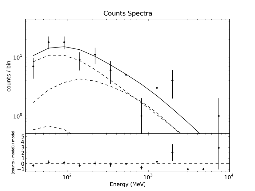
Figure 15: Fitted counts spectrum and residuals for the data shown in Fig. 14. The contributions of the three model components are plotted as the long dashed curves, and from top to bottom, are the Galactic diffuse, extragalactic diffuse, and point source. The solid curve is the sum of the three components.

Figure 16: Change in the log-likelihood as a function of GRB flux for $E>100$ MeV. The horizontal dashed line indicate the 95% CL corresponding to an upper-limit of $1.3\times 10^{-5}$ ph cm^-2 s^-1.

To check the method’s validity, we ran Monte Carlo simulations under the same observing conditions and using the source model and best-fit parameters from the likelihood analysis as inputs, and we analyzed each simulation to find the best-fit flux. The left panel of Fig. 17 shows the distribution of fitted fluxes for these simulations, and the right panel shows the normalized cumulative distribution for these data and the cumulative distribution inferred by computing the corresponding $\chi^{2}$ probability from the profile likelihood curve shown in Fig. 16.

Figure 17: Left: Distribution of fitted fluxes for the point source representing the GRB derived from 766 LAT simulations using the best-fit model obtained from the original dataset. Right: The solid curve is the normalized cumulative distribution determined from the fitted flux distribution. The dotted curve is the cumulative fraction that would be predicted by the likelihood profile shown in figure 16.

7 Spectral Analysis

To demonstrate the spectral analysis that will be possible with the $Fermi$ data, we present two sample analyses, the first the joint fit of GBM and LAT count spectra, and the second the search for a cutoff in the LAT energy band. In both cases we use transient class LAT counts. In general, bursts are short but bright, and thus we can tolerate the higher background rate of the transient class to increase the number of burst counts. While we focus here on LAT-GBM joint fits, such fits will also be possible between the $Fermi$ detectors and those of other missions, such as Swift (Stamatikos et al., 2008a; Band, 2008).

7.1 GBM and LAT Combined Analysis

In this example, we assume that a simulated burst was detected and localized by the GBM. Analysis of the LAT data found 160 transient event class photons in a 20^∘ region surrounding the GBM position during the 3 s prompt phase observed by the GBM; the Automated Science Processing (ASP) that will be run after the LAT events are reconstructed (§3.2) localized the burst with an uncertainty radius of $0.05^{\circ}$. Fig. 18 shows the GBM and LAT light curves.

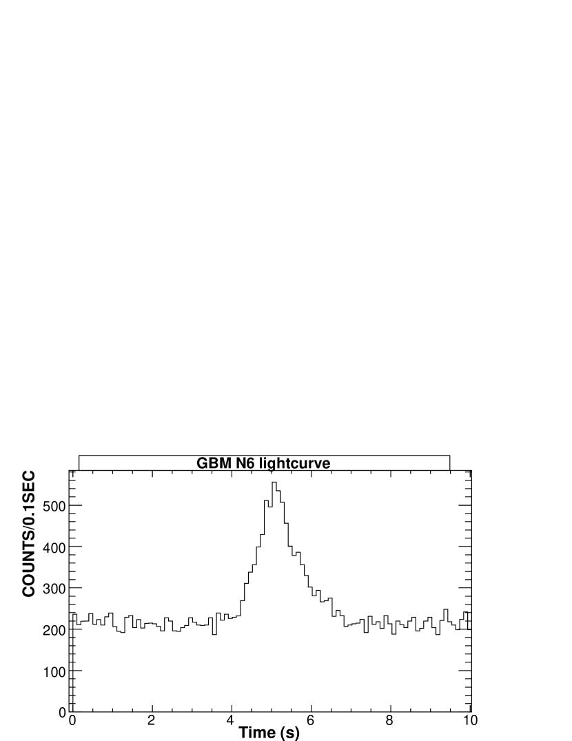
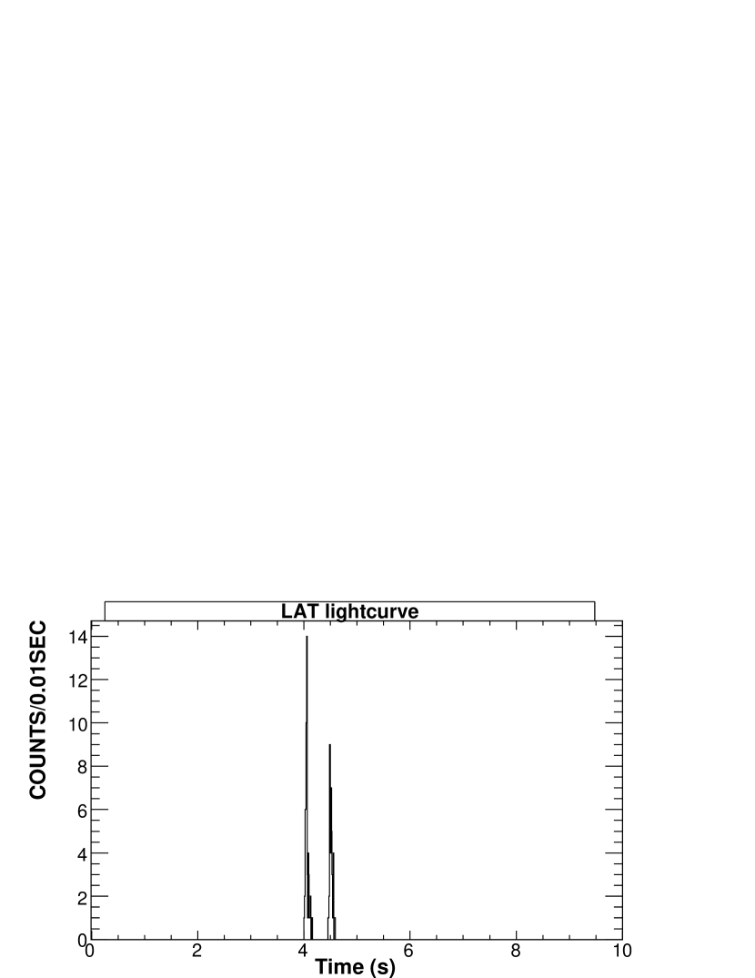
Figure 18: GBM NaI (left) and LAT (right) light curves of the prompt emission from the simulated burst.

The simulated GBM and LAT data, both event lists, were accumulated over the burst’s prompt phase, and the LAT events were binned into 10 energy bins. Two NaI and one BGO detector provided count spectra. The GBM background spectra used to simulate the counts were used as the background for the GBM count spectra, while the LAT data were assumed not to be contaminated by background events. We performed a joint fit to the 4 count spectra (from 2 NaI, one BGO and the LAT detectors) with the standard X-ray analysis tool XPSEC using the Cash statistic (Cash, 1979). The ‘Band’ spectrum (eq. 1) was used to create the simulated data and for the joint fit. Fig. 19 shows the simulated data (with error bars) and best-fit model (histogram). The fit yielded $\alpha=-0.97\pm 0.05$ (input value of $-1.09$) and $\beta=-1.80\pm 0.01$ (input value of $-1.90$).

Figure 19: Photon spectrum of the simulated burst: in the top panel, crosses show the data of the different sub-detectors (two NaI detectors in black and red, one BGO in green, and the LAT in blue) and the histogram denotes the best fit of a Band function. The bottom panel shows the ratio of the simulated data to the fit model.

Thus $Fermi$ will measure the energy spectrum of bursts over 7 orders of magnitude in energy through its combination of detectors. The energy bands of the NaI and BGO detectors overlap in the energy region of the peak energy, and the BGO and the LAT energy bands also overlap.

7.2 Study of GRB high-energy properties with the LAT

Whether the burst spectrum is a simple power law in the LAT energy band, or has a cutoff spectrum is of great theoretical interest (see § 2.2.2). Therefore, we simulated and then fit spectra with such cutoffs to determine if they would be detectable.

We used the simulation software described in § 4.1 to simulate 5 years of $Fermi$ observations. In this simulation, the temporal and spectral properties of GRBs were based on a phenomenological or physical model, including not only synchrotron emission but also inverse Compton emission for a few bursts. The simulated spectra did not have any intrinsic cutoffs, but included gamma-ray absorption by the Extragalactic Background Light (EBL) between the burst and the Earth, following the model of Kneiske et al. (2004). This extrinsic cut-off only appears at the highest energies (at least 10 GeV), depending on the distance of the bursts.

The search for high-energy cut-offs was performed using only simulated LAT data. First we selected those bursts that have no inverse Compton component, and more than 20 LAT counts. Each count spectrum was fit both by a simple power law and by a power law with an exponential cutoff with characteristic energy $E_{c}$.

The likelihoods of the resulting fits were examined to evaluate the improvement of the fit by adding the cutoff (one additional parameter). The difference of the likelihoods follows a $\chi^{2}$-distribution with one degree of freedom, with the null hypothesis probability distribution shown in Fig. 20. Two bursts exhibit a very small probability of being consistent with no cutoff, and thus we consider these bursts to have a statistically significant high-energy cutoff. While both bursts have average redshifts (1.71 and 3.35) compared to the full sample, they are very bright, with more than 1000 photons detected.

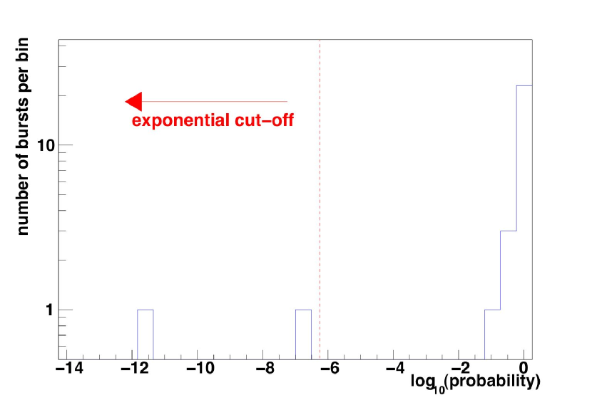
Figure 20: $\chi^{2}$-probability of the difference of the likelihoods of fits of a power law with and without an exponential cutoff: a probability of $<5.7\times 10^{-7}$ corresponds to a 5$\sigma$ detection of a cutoff.

For these two bursts we performed a second fit using the parameterisation of the EBL cut-off proposed by Reyes (2007) where the cutoff is $\exp(-\tau)$, with $\tau=1+(E-E_{1})/P$ for $E>E_{1}-P$, and $0$ otherwise; $E_{1}$ is the redshift-dependent energy where the optical depth is unity, and $P$ is a redshift-dependent energy scaling factor. The two fitted values of $E_{1}$ ($51.5^{+6.7}_{-3.6}$ GeV and $43.5^{+31.0}_{-10.0}$ GeV), are in good agreement with the true values ($46.6$ GeV and $30.7$ GeV) of the model used for the simulation. Thus the LAT will be sensitive to cutoffs in the brightest bursts, with good spectral reconstruction.

8 Coordination with Other Burst Missions

8.1 Coordination with Swift

The $Fermi$ detectors will provide few localizations accurate to less than 10 arcmin that are necessary for the optical followups that can determine redshifts. On the other hand, the Swift instruments (Gehrels et al., 2004)—the Burst Alert Telescope (BAT), the X-Ray Telescope (XRT) and the Ultraviolet-Optical Telescope (UVOT)—provide progressively better burst localizations that are rapidly disseminated by the GRB Coordinate Network (GCN), resulting in multiwavelength followup observations and frequently burst redshifts. However, the BAT’s 15–150 keV energy band is often insufficient to determine the spectrum of the prompt burst emission, particularly $E_{p}$, the ‘peak energy’ where most of the burst energy is radiated (see § 4.1); $E_{p}$ is important not only for burst energetics but also for reported relationships between intrinsic burst parameters (Amati, 2006; Ghirlanda et al., 2004; Firmani et al., 2006) that may turn bursts into standard candles. And for those bursts where the BAT can determine $E_{p}$, Swift cannot determine whether there is a second emission component above the 15–150 keV band (as discussed in §2.2). In addition, Swift’s burst afterglow observations ‘only’ extend to the X-ray band ($E<10$ keV); as discussed in § 2.1, EGRET detected GeV-band prompt and afterglow emissions (Hurley et al., 1994; Dingus, 2003). Thus $Fermi$ and Swift capabilities complement each other (Stamatikos et al., 2008a); between the UVOT, XRT, BAT, GBM and LAT, the two mission’s observations span 11 energy decades.

The $Fermi$ and Swift missions are working to increase the number of bursts that are observed simultaneously by the BAT and the LAT; this will increase the number of bursts with localizations, redshifts, spectra and optical through gamma-ray afterglows. Simultaneous burst observations by $Fermi$ and other burst missions (e.g., AGILE, INTEGRAL, Konus-Wind, RHESSI, Suzaku-WAM) will also complement each other and permit cross-calibration, but Swift’s pointing is the most flexible (Band, 2008).

$Fermi$’s and Swift’s low earth orbits (altitudes of $\sim$565 and $\sim$590 km, respectively) are inclined to the Earth’s equator by 25.6^∘ and 20.6^∘, respectively. The two orbits will beat with a period of $\sim$13 days, that is, the two missions will be on the same side, or opposite sides, of the Earth with a nearly two week period. Because of the uniformity of the LAT’s sky-exposure and the large FOVs of the BAT and the LAT, the relative inclination of the two orbits (which can be as small as 5^∘ or as large as 46^∘) has little effect on the overlap of the FOVs. The relative inclination varies with a period of approximately 6.5 years.

In general $Fermi$ will survey the sky, pointing the LAT 35^∘ above or below the orbital plane (as described in § 3). On the other hand, every orbit Swift points the Narrow-Field Instruments (NFIs—the XRT and UVOT) at a number of targets that satisfy the mission’s observational constraints: the NFIs cannot be pointed near the Sun, moon, horizon or ram direction; anti-Sun observations are preferred to increase the detection of bursts during Earth’s night. Since $Fermi$’s observing mode will not change, but Swift’s timeline is by design extremely flexible, increasing the overlap between the mission’s FOVs, and thus increasing the number of simultaneous burst detections, will be done through Swift’s targeting. Between following-up bursts the Swift NFIs are used for other observation programs (and will observe $Fermi$ sources). By choosing NFI targets at times that will increase the LAT-BAT overlap, we estimate that this overlap can be improved by a factor of $\sim$2 without sacrificing Swift’s science objectives. Note that increasing the BAT-LAT overlap will by necessity increase the overlap between the BAT and GBM.

Swift detects $\sim$100 bursts per year, and approximately one LAT detection per month is anticipated, although this prediction of the LAT’s detection rate is based on extrapolations from lower energy (see § 5.2). Given the differences in the detectability of typical bursts, we assume that Swift’s BAT will detect all the bursts that the LAT will detect when the burst is in both their FOVs The LAT’s larger FOV compensates for the BAT’s greater ability to detect typical bursts, resulting in comparable detection rates. Based on a number of modeling assumptions, and assuming that Swift’s targeting can increase the overlap of the BAT and LAT FOVs by $\times$2, we estimate $\sim$10 BAT bursts per year with LAT detections or upper limits, and $\sim$4 LAT bursts per year with BAT detections. We emphasize that our estimates of the LAT detection rate assumes that the 10–1000 keV component observed by BATSE, BAT and now the GBM extrapolates unbroken into the LAT’s energy band.

8.2 TeV Observations

The synergy between $Fermi$ and ground-based telescopes operating above a few tens of GeV will expand the study of the still-unknown spectral and temporal properties of GRBs above a few GeV. Extending the analysis of burst temporal and spectral properties to even higher energies would have a large impact on the knowledge of the particle acceleration and emission processes occurring in the burst environment. High energy spectra would probe the distant Universe, revealing the universe’s transparency to high-energy gamma-rays and measuring EBL. The requirements for a good coordination of $Fermi$ with TeV observatories are quite simple, and we examine the potential of such simultaneous observations in terms of expected rates of alerts and sensitivity.

Major TeV observatories operate above $\sim$100 GeV (or somewhat lower for the next generation of instruments), and Imaging Atmospheric Cherenkov Telescopes (IACTs) have a sensitivity of $10^{-11}$ to $10^{-9}$ erg cm^-2 to the latter part of the prompt phase and early afterglow emission of GRBs (i.e., from $\sim$10 s to a few hours after the trigger time). The observatories’ duty cycle, FOV and sky coverage will determine their response to $Fermi$ alerts. With a high duty cycle ($\sim$100%) and a good sky coverage ($\sim$20%), ground arrays like MILAGRO and ARGO will be able to react to any alert provided by the GBM or the LAT. In contrast, IACTs like CANGAROO, HESS, MAGIC, VERITAS, or STACEE have a low duty cycle ($\sim$10%) because they observe only during clear and moonless nights, but they can slew to any location within a few minutes and access $\sim$20% of the sky. Because of their small FOV ($\sim$5^∘), IACTs will require a GRB position accuracy of $\pm$1^∘ and thus will respond effectively to LAT alerts only.

Using a phenomenological model to describe GRB properties in the LAT range, we combine the estimated GRB detection rate (1 GRB per month) with the above duty cycle and sky coverage to compute the possible joint observations by $Fermi$ and TeV experiments. $Fermi$ should provide $\sim$40 alerts (including 2 to 5 LAT alerts) per year during the prompt burst phase, that ground arrays will be able to follow up. Few of them will be followed-up by IACTs due to localization accuracy and to observing time constraints.The LAT detected bursts per year suitable for TeV followup should be considered as the highest priority targets in TeV telescope plans. A few afterglows per year may be also followed-up by IACTs, while ground arrays will probably be much less sensitive to afterglows.

8.3 Neutrino Observations

A major step forward in understanding of the microphysics of the GRB central engines might be achieved via the detection of non-electromagnetic emission such as gravitational waves (Abbott et al., 2005) and neutrinos. Because they are weakly-interacting, neutrinos are unique (albeit elusive) cosmic messengers because they are not absorbed nor deflected on their way to the observer. The viability of high energy neutrino astronomy (Gaisser et al., 1995) opens a new observing channel that complements the high energy electromagnetic spectrum that will be probed directly by the LAT.

Hadronic fireball models (§2.2.1), predict a taxonomy of correlated MeV to EeV neutrinos of varying flavor and arrival times. Ideal for detection are $\sim$TeV-PeV muon neutrinos (Waxman & Bahcall, 1997) produced as the leptonic decay products of photomeson interactions $\left(p+\gamma\rightarrow\Delta^{+}\rightarrow\pi^{+}+[n]\rightarrow\mu^{+}+\nu_{\mu}\rightarrow e^{+}+\nu_{e}+\bar{\nu}_{\mu}+\nu_{\mu}\right)$ within the internal shocks of the relativistic fireball. Since the prompt gamma rays act as the ambient photon target field, the burst neutrinos are expected to be spatially and temporally coincident with the gamma-ray emission. Therefore Antarctic Cherenkov telescopes such as Antarctic Muon and Neutrino Detector Array (AMANDA) (Ahrens et al., 2002) and IceCube (Ahrens et al., 2004) can perform a nearly background-free search for burst neutrinos correlated with the prompt gamma-ray emission (Stamatikos et al., 2005; Stamatikos & Band, 2006). Neutrino telescopes have FOVs determined by their position on the Earth, and accumulate and preserve their data, and therefore need not to respond to bursts in realtime. Instead, the neutrino data archived is searched periodically for neutrinos correlated with the time and position of prompt burst emission. Analysis of AMANDA data has resulted in the most stringent upper limits upon correlated multi-flavored neutrino emission from GRBs (Achterberg et al., 2007, 2008). AMANDA’s km-scale successor, IceCube, is currently under construction with anticipated completion by $\sim$2010, and thus will operate during the $Fermi$ era.

9 Conclusions and Future Work

In this paper we provided an overview of the LAT’s capabilities to reveal the rich burst phenomenology in the $>$100 MeV band at which the EGRET observations merely hinted, and which theoretical scenarios predict. These capabilities can be realized only through efficient analysis techniques and software. In this final section we discuss the future analysis development that we anticipate during the early part of the $Fermi$ mission.

Burst triggers are applied to the LAT data both onboard and on-ground. The onboard trigger contends with a higher non-burst background rate, but can provide burst notifications and localizations within tens of seconds after the burst, while the on-ground trigger is more sensitive because the background can be reduced, but the burst notification and localizations have a $\sim$3 hr latency. The thresholds for both triggers depend on the actual instrument response and background rates that are only now being evaluated. Thus during the mission’s early phase we will tune the detection algorithms to minimize false triggers and maximize the detection sensitivity.

In particular, we are investigating various ‘cuts’ of the reconstructed events used by the on-ground detection algorithms. These cuts do not merely increase or decreased the effective area and the background rate, but also change their energy dependence. Relative changes in the effective area and background rate affect the detectability of bursts of different durations, since the background is less important for detecting short bursts.

The GBM and LAT spectra will be analyzed jointly, giving spectral fits from $\sim$8 keV to over 300 GeV, a bandpass of up to 7.5 energy decades. Typically the spectral analysis will fit the parameters of functional forms such as the ‘Band’ function.

However, given the theoretical uncertainties in the underlying GRB spectrum in the LAT band (e.g., the unknown high energy attenuation by the EBL and intrinsic photon fields), we will explore model-independent spectral reconstruction. Deconvolution of instrument response effects in the Poisson statistics regime is notoriously difficult, but there have been advances in recent years. For example, Nowak & Kolaczyk (2000) derived a Bayesian multiscale framework that is inspired by wavelet methods, but adapted for Poisson statistics; using these methods, they reconstructed a Solar flare emission line spectrum observed by CGRO’s COMPTEL. D’Agostini (1995) derived another Bayesian iterative method for deconvolving spectra; uncertainties on the unfolded distribution can be estimated from a covariance matrix.

Thus we anticipate an exciting mission exploring new burst phenomena and developing the techniques to extract the maximum information from the LAT.

References

- Abbott et al. (2005) Abbott, B., et al. 2005, Phys. Rev. D, 72, 042002
- Abdo et al. (2009) Abdo, A., et al. 2009, Science, 323, 1688
- Achterberg et al. (2007) Achterberg, A., et al. 2007, Ap. J., 664, 397
- Achterberg et al. (2008) —. 2008, Ap. J., 674, 357
- Agostinelli et al. (2003) Agostinelli, S., et al. 2003, Nuclear Instruments and Methods in Physics Research A, 506, 250
- Ahrens et al. (2002) Ahrens, J., et al. 2002, Phys. Rev. D, 66, 012005
- Ahrens et al. (2004) —. 2004, Astroparticle Physics, 20, 507
- Amati (2006) Amati, L. 2006, MNRAS, 372, 233
- Amelino-Camelia et al. (1998) Amelino-Camelia, G., Ellis, J., Mavromatos, N. E., Nanopoulos, D. V., & Sarkar, S. 1998, Nature, 395, 525
- Atwood et al. (2004) Atwood, W., et al. 2004, in Calorimetry in Particle Physics, ed. C. Cecchi, P. Cenci, P. Lubrano, & M. Pepe, 329–336
- Atwood et al. (2009) Atwood, W., et al. 2009, Ap. J., 697, 1071
- Bahcall & Mészáros (2000) Bahcall, J. N., & Mészáros, P. 2000, Physical Review Letters, 85, 1362
- Baldini et al. (2006) Baldini, L., et al. 2006, Nucl. Phys. Proc. Suppl., 150, 62
- Band (2003) Band, D. 2003, Ap.J., 588, 945
- Band et al. (1993) Band, D., Matteson, J., Ford, L., Schaefer, B., Palmer, D., Teegarden, B., Cline, T., Briggs, M., Paciesas, W., Pendleton, G., Fishman, G., Kouveliotou, C., Meegan, C., Wilson, R., & Lestrade, P. 1993, Ap. J., 413, 281
- Band (2007) Band, D. L. 2007, in American Institute of Physics Conference Series, Vol. 921, The First GLAST Symposium, ed. S. Ritz, P. Michelson, & C. A. Meegan, 446–447
- Band (2008) Band, D. L. 2008, in American Institute of Physics Conference Series, Vol. 1000, American Institute of Physics Conference Series, 121–124
- Baring (2006) Baring, M. G. 2006, Ap. J., 650, 1004
- Baring & Braby (2004) Baring, M. G., & Braby, M. L. 2004, Ap. J., 613, 460
- Baring & Harding (1997) Baring, M. G., & Harding, A. K. 1997, Ap. J. Lett., 481, L85+
- Battelino et al. (2007a) Battelino, M., Ryde, F., Omodei, N., & Band, D. L. 2007a, in American Institute of Physics Conference Series, Vol. 921, American Institute of Physics Conference Series, ed. S. Ritz, P. Michelson, & C. A. Meegan, 478–479
- Battelino et al. (2007b) Battelino, M., Ryde, F., Omodei, N., & Longo, F. 2007b, in American Institute of Physics Conference Series, Vol. 906, American Institute of Physics Conference Series, ed. M. Axelsson & F. Ryde, 28–39
- Boggs et al. (2004) Boggs, S. E., Wunderer, C. B., Hurley, K., & Coburn, W. 2004, Ap. J. Lett., 611, L77
- Bottcher & Dermer (1998) Bottcher, M., & Dermer, C. D. 1998, Ap. J. Lett., 499, L131+
- Bouvier et al. (2008) Bouvier, A., Band, D., Bregeon, J., Chiang, J., Cutini, S., Dingus, B., Gehrels, N., Fukazawa, Y., Hayashida, M., Longo, F., McEnery, J., Ohno, M., Omodei, N., Pelassa, V., Piron, F., Sanchez, D., Scargle, J., Tajima, H., Tanaka, T., & Thayer, G. 2008, GRB Coordinates Network, 8183, 1
- Briggs (1999) Briggs, M. S. 1999, in Astronomical Society of the Pacific Conference Series, Vol. 190, Gamma-Ray Bursts: The First Three Minutes, ed. J. Poutanen & R. Svensson, 133–+
- Bromm & Loeb (2006) Bromm, V., & Loeb, A. 2006, Ap. J., 642, 382
- Burnett (2007) Burnett, T. H. 2007, in American Institute of Physics Conference Series, Vol. 921, American Institute of Physics Conference Series, ed. S. Ritz, P. Michelson, & C. A. Meegan, 530–531
- Cash (1979) Cash, W. 1979, Ap. J., 228, 939
- Coppi & Aharonian (1997) Coppi, P. S., & Aharonian, F. A. 1997, Ap. J. Lett., 487, L9+
- Crider et al. (1997) Crider, A., Liang, E. P., Smith, I. A., Preece, R. D., Briggs, M. S., Pendleton, G. N., Paciesas, W. S., Band, D. L., & Matteson, J. L. 1997, Ap. J. Lett., 479, L39+
- D’Agostini (1995) D’Agostini, G. 1995, Nuclear Instruments and Methods in Physics Resarch A, 362, 487
- Davis et al. (1994) Davis, S. P., Norris, J. P., Kouveliotou, C., Fishman, G. J., Meegan, C. A., & Paciesas, W. S. 1994, in American Institute of Physics Conference Series, Vol. 307, Gamma-Ray Bursts, ed. G. J. Fishman, 182–+
- de Jager & Stecker (2002) de Jager, O. C., & Stecker, F. W. 2002, Ap. J., 566, 738
- Derishev et al. (2000) Derishev, E. V., Kocharovsky, V. V., & Kocharovsky v., V. 2000, in American Institute of Physics Conference Series, Vol. 526, Gamma-ray Bursts, 5th Huntsville Symposium, ed. R. M. Kippen, R. S. Mallozzi, & G. J. Fishman, 460–464
- Dermer (2007) Dermer, C. D. 2007, ArXiv Astrophysics e-prints
- Dermer & Atoyan (2004) Dermer, C. D., & Atoyan, A. 2004, Astron. & Astrophys., 418, L5
- Dermer et al. (2000) Dermer, C. D., Chiang, J., & Mitman, K. E. 2000, Ap. J., 537, 785
- Dingus (2003) Dingus, B. L. 2003, in American Institute of Physics Conference Series, Vol. 662, Gamma-Ray Burst and Afterglow Astronomy 2001: A Workshop Celebrating the First Year of the HETE Mission, ed. G. R. Ricker & R. K. Vanderspek, 240–243
- Fan et al. (2008) Fan, Y.-Z., Piran, T., Narayan, R., & Wei, D.-M. 2008, Mon. Not. RAS, 384, 1483
- Fan et al. (2005) Fan, Y. Z., Zhang, B., & Wei, D. M. 2005, Ap. J., 629, 334
- Fenimore et al. (1995) Fenimore, E. E., in ’t Zand, J. J. M., Norris, J. P., Bonnell, J. T., & Nemiroff, R. J. 1995, Ap. J. Lett., 448, L101+
- Firmani et al. (2006) Firmani, C., Ghisellini, G. andAvila-Reese, V., & Ghirlanda, G. 2006, MNRAS, 370, 185
- Foley et al. (2008) Foley, S., McGlynn, S., Hanlon, L., McBreen, S., & McBreen, B. 2008, Astron. & Astrophys., 484, 143
- Ford et al. (1995) Ford, L. A., Band, D. L., Matteson, J. L., Briggs, M. S., Pendleton, G. N., Preece, R. D., Paciesas, W. S., Teegarden, B. J., Palmer, D. M., Schaefer, B. E., Cline, T. L., Fishman, G. J., Kouveliotou, C., Meegan, C. A., Wilson, R. B., & Lestrade, J. P. 1995, Ap. J., 439, 307
- Fragile et al. (2004) Fragile, P. C., Mathews, G. J., Poirier, J., & Totani, T. 2004, Astroparticle Physics, 20, 591
- Gaisser et al. (1995) Gaisser, T. K., Halzen, F., & Stanev, T. 1995, Physics Reports, 258, 173
- Galli & Guetta (2008) Galli, A., & Guetta, D. 2008, Astron. & Astrophys., 480, 5
- Galli & Piro (2007) Galli, A., & Piro, L. 2007, Astron. & Astrophys., 475, 421
- Gehrels et al. (2004) Gehrels, N., Chincarini, G., Giommi, P., Mason, K. O., Nousek, J. A., Wells, A. A., White, N. E., Barthelmy, S. D., Burrows, D. N., Cominsky, L. R., Hurley, K. C., Marshall, F. E., Mészáros, P., Roming, P. W. A., Angelini, L., Barbier, L. M., Belloni, T., Campana, S., Caraveo, P. A., Chester, M. M., Citterio, O., Cline, T. L., Cropper, M. S., Cummings, J. R., Dean, A. J., Feigelson, E. D., Fenimore, E. E., Frail, D. A., Fruchter, A. S., Garmire, G. P., Gendreau, K., Ghisellini, G., Greiner, J., Hill, J. E., Hunsberger, S. D., Krimm, H. A., Kulkarni, S. R., Kumar, P., Lebrun, F., Lloyd-Ronning, N. M., Markwardt, C. B., Mattson, B. J., Mushotzky, R. F., Norris, J. P., Osborne, J., Paczynski, B., Palmer, D. M., Park, H.-S., Parsons, A. M., Paul, J., Rees, M. J., Reynolds, C. S., Rhoads, J. E., Sasseen, T. P., Schaefer, B. E., Short, A. T., Smale, A. P., Smith, I. A., Stella, L., Tagliaferri, G., Takahashi, T., Tashiro, M., Townsley, L. K., Tueller, J., Turner, M. J. L., Vietri, M., Voges, W., Ward, M. J., Willingale, R., Zerbi, F. M., & Zhang, W. W. 2004, Ap.J., 611, 1005
- Ghirlanda et al. (2004) Ghirlanda, G., Ghisellini, G., & Lazzati, D. 2004, Ap. J., 616, 331
- Giuliani et al. (2008) Giuliani, A., Mereghetti, S., Fornari, F., Del Monte, E., Feroci, M., Marisaldi, M., Esposito, P., Perotti, F., Tavani, M., Argan, A., Barbiellini, G., Boffelli, F., Bulgarelli, A., Caraveo, P., Cattaneo, P. W., Chen, A. W., Costa, E., D’Ammando, F., di Cocco, G., Donnarumma, I., Evangelista, Y., Fiorini, M., Fuschino, F., Galli, M., Gianotti, F., Labanti, C., Lapshov, I., Lazzarotto, F., Lipari, P., Longo, F., Morselli, A., Pacciani, L., Pellizzoni, A., Piano, G., Picozza, P., Prest, M., Pucella, G., Rapisarda, M., Rappoldi, A., Soffitta, P., Trifoglio, M., Trois, A., Vallazza, E., Vercellone, S., Zanello, D., Salotti, L., Cutini, S., Pittori, C., Preger, B., Santolamazza, P., Verrecchia, F., Gehrels, N., Page, K., Burrows, D., Rossi, A., Hurley, K., Mitrofanov, I., & Boynton, W. 2008, Astron. & Astrophys., 491, L25
- González et al. (2003) González, M. M., Dingus, B. L., Kaneko, Y., Preece, R. D., Dermer, C. D., & Briggs, M. S. 2003, Nature, 424, 749
- Granot et al. (2008) Granot, J., Cohen-Tanugi, J., & do Couto e Silva, E. 2008, Ap. J., 677, 92
- Granot & Guetta (2003) Granot, J., & Guetta, D. 2003, Ap. J. Lett., 598, L11
- Granot et al. (2006) Granot, J., Königl, A., & Piran, T. 2006, Mon. Not. RAS, 370, 1946
- Guetta & Granot (2003) Guetta, D., & Granot, J. 2003, Ap. J., 585, 885
- Guetta & Piran (2005) Guetta, D., & Piran, T. 2005, Astron. & Astrophys., 435, 421
- Gupta & Zhang (2007) Gupta, N., & Zhang, B. 2007, Mon. Not. RAS, 380, 78
- Hafizi & Mochkovitch (2007) Hafizi, M., & Mochkovitch, R. 2007, Astron. & Astrophys., 465, 67
- Hakkila et al. (2007) Hakkila, J., Giblin, T. W., Young, K. C., Fuller, S. P., Peters, C. D., Nolan, C., Sonnett, S. M., Haglin, D. J., & Roiger, R. J. 2007, Ap. J. Supp., 169, 62
- Hoover et al. (2005) Hoover, A. S., Kippen, R. M., & McConnell, M. L. 2005, Nuovo Cimento C Geophysics Space Physics C, 28, 825
- Hurley et al. (1994) Hurley, K., Dingus, B. L., Mukherjee, R., Sreekumar, P., Kouveliotou, C., Meegan, C., Fishman, G. J., Band, D., Ford, L., Bertsch, D., Cline, T., Fichtel, C., Hartman, R., Hunter, S., Thompson, D. J., Kanbach, G., Mayer-Hasselwander, H., von Montigny, C., Sommer, M., Lin, Y., Nolan, P., Michelson, P., Kniffen, D., Mattox, J., Schneid, E., Boer, M., & Niel, M. 1994, Nature, 372, 652
- Jackson et al. (2003) Jackson, B., Scargle, J. D., Barnes, D., Arabhi, S., Alt, A., Gioumousis, P., Gwin, E., Sangtrakulcharoen, P., Tan, L., & Tsai, T. T. 2003, ArXiv Mathematics e-prints
- Kaneko et al. (2008) Kaneko, Y., González, M. M., Preece, R. D., Dingus, B. L., & Briggs, M. S. 2008, Ap. J., 677, 1168
- Kaneko et al. (2006) Kaneko, Y., Preece, R. D., Briggs, M. S., Paciesas, W. S., Meegan, C. A., & Band, D. L. 2006, Ap. J. Supp., 166, 298
- Kashlinsky (2005) Kashlinsky, A. 2005, Ap. J. Lett., 633, L5
- Kneiske et al. (2004) Kneiske, T. M., Bretz, T., Mannheim, K., & Hartmann, D. H. 2004, Astron. & Astrophys., 413, 807
- Kobayashi et al. (2007) Kobayashi, S., Zhang, B., Mészáros, P., & Burrows, D. 2007, Ap. J., 655, 391
- Kocevski & Liang (2003) Kocevski, D., & Liang, E. 2003, Ap. J., 594, 385
- Kouveliotou et al. (1994) Kouveliotou, C., Preece, R., Bhat, N., Fishman, G. J., Meegan, C. A., Horack, J. M., Briggs, M. S., Paciesas, W. S., Pendleton, G. N., Band, D., Matteson, J., Palmer, D., Teegarden, B., & Norris, J. P. 1994, Ap. J. Lett., 422, L59
- Kuehn et al. (2007) Kuehn, F., Bonnell, J., Hughes, R., Norris, J., Ritz, S., Russell, J., Smith, P., & Winer, B. 2007, in American Institute of Physics Conference Series, Vol. 921, American Institute of Physics Conference Series, ed. S. Ritz, P. Michelson, & C. A. Meegan, 556–557
- Liang et al. (2006) Liang, E.-W., Zhang, B.-B., Stamatikos, M., Zhang, B., Norris, J., Gehrels, N., Zhang, J., & Dai, Z. G. 2006, Ap. J. Lett., 653, L81
- Lithwick & Sari (2001) Lithwick, Y., & Sari, R. 2001, Ap. J., 555, 540
- Mattingly (2005) Mattingly, D. 2005, Living Reviews in Relativity, 8, 5
- Mattox et al. (1996) Mattox, J. R., Bertsch, D. L., Chiang, J., Dingus, B. L., Digel, S. W., Esposito, J. A., Fierro, J. M., Hartman, R. C., Hunter, S. D., Kanbach, G., Kniffen, D. A., Lin, Y. C., Macomb, D. J., Mayer-Hasselwander, H. A., Michelson, P. F., von Montigny, C., Mukherjee, R., Nolan, P. L., Ramanamurthy, P. V., Schneid, E., Sreekumar, P., Thompson, D. J., & Willis, T. D. 1996, Astrophysical Journal v.461, 461, 396
- Mészáros & Rees (1994) Mészáros, P., & Rees, M. J. 1994, Mon. Not. RAS, 269, L41+
- Mészáros et al. (1994) Mészáros, P., Rees, M. J., & Papathanassiou, H. 1994, Ap. J., 432, 181
- Neyman & Pearson (1928) Neyman, J., & Pearson, E. 1928, Biometrika
- Norris (2002) Norris, J. P. 2002, Ap. J., 579, 386
- Norris & Bonnell (2006) Norris, J. P., & Bonnell, J. T. 2006, Ap. J., 643, 266
- Norris et al. (2000) Norris, J. P., Marani, G. F., & Bonnell, J. T. 2000, Ap. J., 534, 248
- Norris et al. (1996) Norris, J. P., Nemiroff, R. J., Bonnell, J. T., Scargle, J. D., Kouveliotou, C., Paciesas, W. S., Meegan, C. A., & Fishman, G. J. 1996, Ap. J., 459, 393
- Nousek et al. (2006) Nousek, J. A., Kouveliotou, C., Grupe, D., Page, K. L., Granot, J., Ramirez-Ruiz, E., Patel, S. K., Burrows, D. N., Mangano, V., Barthelmy, S., Beardmore, A. P., Campana, S., Capalbi, M., Chincarini, G., Cusumano, G., Falcone, A. D., Gehrels, N., Giommi, P., Goad, M. R., Godet, O., Hurkett, C. P., Kennea, J. A., Moretti, A., O’Brien, P. T., Osborne, J. P., Romano, P., Tagliaferri, G., & Wells, A. A. 2006, Ap. J., 642, 389
- Nowak & Kolaczyk (2000) Nowak, R. D., & Kolaczyk, E. D. 2000, IEEE Transactions on Information Theory, 46, 1811
- Omodei (2005) Omodei, N. 2005, in High Energy Gamma-ray Experiments, ed. A. De Angelis & O. Mansutti, 189–196
- Omodei (2008) Omodei, N. 2008, GRB Coordinates Network, 8407, 1
- Omodei & Norris (2007) Omodei, N., & Norris, J. 2007, in American Institute of Physics Conference Series, Vol. 921, American Institute of Physics Conference Series, ed. S. Ritz, P. Michelson, & C. A. Meegan, 472–475
- Omodei et al. (2007) Omodei, N., et al. 2007, AIP Conf. Proc., 906, 1
- Paciesas et al. (1999) Paciesas, W. S., Meegan, C. A., Pendleton, G. N., Briggs, M. S., Kouveliotou, C., Koshut, T. M., Lestrade, J. P., McCollough, M. L., Brainerd, J. J., Hakkila, J., Henze, W., Preece, R. D., Connaughton, V., Kippen, R. M., Mallozzi, R. S., Fishman, G. J., Richardson, G. A., & Sahi, M. 1999, Ap. J. Supp., 122, 465
- Panaitescu et al. (1998) Panaitescu, A., Mészáros, P., & Rees, M. J. 1998, Ap. J., 503, 314
- Piran (1999) Piran, T. 1999, Physics Reports, 314, 575
- Pollock et al. (1985) Pollock, A. M. T., Bennett, K., Bignami, G. F., Bloemen, J. B. G. M., Buccheri, R., Caraveo, P. A., Hermsen, W., Kanbach, G., Lebrun, F., Mayer-Hasselwander, H. A., & Strong, A. W. 1985, Astron. & Astrophys., 146, 352
- Pollock et al. (1981) Pollock, A. M. T., Masnou, J. L., Bignami, G. F., Hermsen, W., Swanenburg, B. N., Kanbach, G., Lichti, G. G., & Wills, R. D. 1981, Astron. & Astrophys., 94, 116
- Porciani & Madau (2001) Porciani, C., & Madau, P. 2001, Ap. J., 548, 522
- Preece et al. (2002) Preece, R. D., Briggs, M. S., Giblin, T. W., Mallozzi, R. S., Pendleton, G. N., Paciesas, W. S., & Band, D. L. 2002, Ap. J., 581, 1248
- Preece et al. (1998) Preece, R. D., Briggs, M. S., Mallozzi, R. S., Pendleton, G. N., Paciesas, W. S., & Band, D. L. 1998, Ap. J. Lett., 506, L23
- Preece et al. (2000) —. 2000, Ap. J. Supp., 126, 19
- Rees & Mészáros (2005) Rees, M. J., & Mészáros, P. 2005, Ap. J., 628, 847
- Reyes (2007) Reyes, L. C. 2007, in American Institute of Physics Conference Series, Vol. 921, American Institute of Physics Conference Series, ed. S. Ritz, P. Michelson, & C. A. Meegan, 359–360
- Ryde (2004) Ryde, F. 2004, Ap. J., 614, 827
- Ryde (2005) —. 2005, Ap. J. Lett., 625, L95
- Scargle (1998) Scargle, J. D. 1998, Ap. J., 504, 405
- Schaefer (1999) Schaefer, B. E. 1999, Physical Review Letters, 82, 4964
- Soderberg et al. (2006) Soderberg, A. M., Kulkarni, S. R., Nakar, E., Berger, E., Cameron, P. B., Fox, D. B., Frail, D., Gal-Yam, A., Sari, R., Cenko, S. B., Kasliwal, M., Chevalier, R. A., Piran, T., Price, P. A., Schmidt, B. P., Pooley, G., Moon, D.-S., Penprase, B. E., Ofek, E., Rau, A., Gehrels, N., Nousek, J. A., Burrows, D. N., Persson, S. E., & McCarthy, P. J. 2006, Nature, 442, 1014
- Sommer et al. (1994) Sommer, M., Bertsch, D. L., Dingus, B. L., Fichtel, C. E., Fishman, G. J., Harding, A. K., Hartman, R. C., Hunter, S. D., Hurley, K., Kanbach, G., Kniffen, D. A., Kouveliotou, C., Lin, Y. C., Mattox, J. R., Mayer-Hasselwander, H. A., Michelson, P. F., von Montigny, C., Nolan, P. L., Schneid, E., Sreekumar, P., & Thompson, D. J. 1994, Ap. J. Lett., 422, L63
- Stamatikos & Band (2006) Stamatikos, M., & Band, D. L. 2006, in American Institute of Physics Conference Series, Vol. 836, Gamma-Ray Bursts in the Swift Era, ed. S. S. Holt, N. Gehrels, & J. A. Nousek, 599–604
- Stamatikos et al. (2008a) Stamatikos, M., Sakamoto, T., & Band, D. L. 2008a, in American Institute of Physics Conference Series, Vol. 1000, American Institute of Physics Conference Series, 133–136
- Stamatikos et al. (2008b) Stamatikos, M., Ukwatta, T. N., Sakamoto, T., Barthelmy, S. D., Norris, J. P., Gehrels, N., & Dhuga, K. S. 2008b, in American Institute of Physics Conference Series, Vol. 1000, American Institute of Physics Conference Series, 137–141
- Stamatikos et al. (2005) Stamatikos, M., et al. 2005, in International Cosmic Ray Conference, Vol. 4, International Cosmic Ray Conference, 471–+
- Tajima et al. (2008) Tajima, H., Bregeon, J., Chiang, J., & Thayer, G. 2008, GRB Coordinates Network, 8246, 1
- Totani (1998) Totani, T. 1998, Ap. J. Lett., 509, L81
- Walker et al. (2000) Walker, K. C., Schaefer, B. E., & Fenimore, E. E. 2000, Ap. J., 537, 264
- Wang et al. (2001) Wang, X. Y., Dai, Z. G., & Lu, T. 2001, Ap. J. Lett., 546, L33
- Wang et al. (2006) Wang, X.-Y., Li, Z., & Mészáros, P. 2006, Ap. J. Lett., 641, L89
- Waxman (1997) Waxman, E. 1997, Ap. J. Lett., 485, L5+
- Waxman & Bahcall (1997) Waxman, E., & Bahcall, J. 1997, Physical Review Letters, 78, 2292
- Wilks (1938) Wilks, S. S. 1938, Ann. Math. Stat., 9, 60
- Xiao & Schaefer (2009) Xiao, L., & Schaefer, B. E. 2009, ArXiv e-prints
- Yi et al. (2006) Yi, T., Liang, E., Qin, Y., & Lu, R. 2006, Mon. Not. RAS, 367, 1751
- Zhang (2007) Zhang, B. 2007, Chinese Journal of Astronomy and Astrophysics, 7, 1
- Zhang & Mészáros (2001) Zhang, B., & Mészáros, P. 2001, Ap. J., 559, 110
- Zhang & Mészáros (2002) —. 2002, Ap. J., 581, 1236