New analytical methods for gravitational radiation and reaction in binaries with arbitrary mass ratio and relative velocity

Abstract

We present a new analytical framework for describing the dynamics of a gravitational binary system with unequal masses moving with arbitrary relative velocity, taking into account the backreaction from both compact objects in the form of tidal deformation, gravitational waves and self forces. Allowing all dynamical variables to interact with each other in a self-consistent manner this formalism ensures that all the dynamical quantities involved are conserved on the background spacetime and obey the gauge invariance under general coordinate transformations that preserve the background geometry. Because it is based on a generalized perturbation theory and the important new emphasis is on the self-consistency of all the dynamical variables involved we call it a gravitational perturbation theory with self-consistent backreaction (GP-SCB).

As an illustration of how this formalism is implemented we construct perturbatively a self-consistent set of equations of motion for an inspiraling gravitational binary, which does not require extra assumptions such as slow motion, weak-field or small mass ratio for its formulation. This case should encompass the inspiral and possibly the plunge and merger phases of binaries with otherwise general parameters (e.g., mass ratio and relative velocity) though more investigation is needed to substantiate it.

In the second part, we discuss how the mass ratio can be treated as a perturbation parameter in the post-Newtonian effective field theory (PN-EFT) approach, thus extending the work of Goldberger and Rothstein for equal mass binaries to variable mass ratios $\eta\equiv m/M$ ($M\geq m$). As the mass ratio $\eta$ decreases from 1 to near 0, the smaller mass can be accelerated to higher speeds thereby requiring higher order post-Newtonian corrections to describe the system with sufficient accuracy for the data analysis requirements of current and future gravitational wave interferometer detectors. We provide rough estimates for the higher post-Newtonian orders needed to determine the number of gravitational wave cycles, with a specified precision, that fall into a detector’s bandwidth. For example, we find that the number of cycles may need to be calculated through 4.5PN for $\sim 5\%$ precision (relative to 2.5PN corrections) for a compact binary with $10M_{\odot}$ and $100M_{\odot}$ constituents.

I Introduction

Ground-based gravitational wave interferometer detectors, such as LIGO Abramovici:LIGO , are currently operating at their intended design sensitivity and are actively constraining the amplitudes of gravitational waves that may be passing within their detectable bandwidth. These observatories are expected to detect gravitational wave signals from the inspiral, plunge, merger and ringdown phases of binaries with astrophysical masses, ranging from the mass of a neutron star to the mass of several hundred solar masses. Space-based detectors, such as LISA LISA , which are currently in the planning and development stages are designed to detect the gravitational waves from inspirals of extreme mass ratio binaries and from binaries with nearly equal and large masses (e.g., with masses $\sim 10^{6}M_{\odot}$), among other sources.

I.1 Existing analytical formalisms for gravitational binaries

Different descriptions of gravitational binary systems ultimately depend on the parameters of the system. For example, the post-Newtonian (PN) approximation (see below) is useful for binaries with nearly equal masses ($\mathrel{\hbox to0.0pt{\lower 3.0pt\hbox{\hskip 1.0pt$\sim$}\hss}\raise 1.0pt\hbox{$<$}}10M_{\odot}$) during the inspiral phase, with extreme mass ratios where the small compact object moves in the weak-field region of the supermassive black hole, and with supermassive black holes orbiting slowly in a weak-field regime. For motion in a strong field, one often uses gravitational perturbation (GP) theory on a fixed but curved background (see below) to describe the perturbations of a small compact object moving in the background field of a supermassive black hole. We review these formalisms in somewhat more detail below.

I.1.1 The post-Newtonian expansion

The post-Newtonian approximation is based on the assumption that two weakly gravitating objects orbit about each other at nonrelativistic speeds on a flat background. The strict weak field requirement can be lifted by constructing an annulus about each compact object where the PN-expanded metric is matched onto the near-field perturbed metric of the strongly gravitating compact object Damour:300yrs ; Thorne:RevModPhys52 .

Iteratively solving for the metric perturbations and the positions of the masses yields approximate expressions in powers of the relative velocity for the phase of the emitted gravitational radiation, the energy and angular momentum they carry, the location of the innermost stable circular orbit, etc. To date, the equations of motion for the compact objects have been computed to order $v^{7}$ beyond the Newtonian ones, also denoted as 3.5PN, for non-spinning compact objects. For good reviews of the PN expansion see Blanchet:LRR ; FutamaseItoh:LRR and Maggiore .

The PN expansion is valid in a region, called the near zone, smaller than the wavelength of the emitted gravitational waves. Applying the PN approximation far from the source (in the far zone) can lead to logarithmic divergences since retardation effects from the finite propagation speed of gravitational waves cannot be neglected far from the sources. As a result, the PN metric in the near zone is matched to a metric containing the gravitational radiation emitted by the binary. This matching is performed in an overlapping region of the near and far zones. In this way, one can describe the generation and propagation of gravitational waves by slowly moving compact objects in the PN framework Thorne:RevModPhys52 ; Damour:300yrs .

The metric in the far zone can be calculated from a post-Minkowski (PM) expansion where the Einstein equations are expanded in powers of Newton’s constant $G_{N}$ and solved iteratively for each order of the metric perturbations. In particular, there is no constraint on the velocities of the sources. This method is valid in those regions of spacetime that are weakly gravitating so the PM expansion is not applicable for compact binaries everywhere in the spacetime. However, as discussed above, the PM expansion can be applied far from such a system by matching onto the perturbed metric of the near zone computed in the PN approximation.

The traditional approaches to the post-Newtonian expansion outlined above have been efficiently streamlined by Goldberger and Rothstein GoldbergerRothstein:PRD73 who borrow time-honored techniques from quantum field theory. For example, Feynman diagrams are utilized to construct the PN expansion order by order and the divergences typically encountered in a theory of interacting fields and point particles are conveniently regularized using dimensional regularization tHooftVeltman:NuclPhysB44 . Furthermore, a systematic formalism is introduced in GoldbergerRothstein:PRD73 that allows for a point particle description of an extended body by utilizing an effective field theory paradigm and including all possible extra terms (so-called non-minimal couplings) into the point particle Lagrangian that are consistent with general coordinate invariance and reparamaterization invariance.

Recent years have seen the development of the so-called effective one-body (EOB) approach BuonannoDamour:PRD59 ; BuonannoDamour:PRD62 that uses the 3PN expanded Hamiltonian to resum the conservative terms by mapping the two-body dynamics onto a system describing a test particle moving in an effective background spacetime. This background is a deformed Schwarzschild spacetime where the deformation parameter is the symmetric mass ratio, $\nu=mM/(m+M)^{2}$. By following the geodesic motion of the test particle on this effective geometry one can describe the conservative dynamics of the binary even in the relativistic regime. The effects of radiation reaction are “grafted” onto the conservative test particle dynamics by using a flux balance argument where the power emitted in gravitational waves equals the loss in the particle’s mechanical energy due to the reactive forces that come from emitting the gravitational radiation.

While the EOB method has proved remarkably successful for providing approximate analytical waveforms of nearly equal mass non-spinning binaries it has several shortcomings from both a practical and theoretical point of view. On the practical side, the EOB approach does not yet describe well the dynamics of spinning binaries. Furthermore, for non-spinning binaries, one must patch the inspiral/plunge phases to the merger and the merger to the ringdown phase because the EOB approach does not smoothly describe these transitions. On the theoretical side, the EOB approach can be regarded as a phenomenological model with parameters that are obtained by fitting to numerical simulations of inspiral waveforms, for example. See Boyle_etal:PRD78 ; DamourNagar:0902.0136 ; Buonanno_etal:0902.0790 and references therein for further discussions.

I.1.2 Black hole perturbation theory for extreme mass ratios

The extreme mass ratio inspiral (EMRI) scenario consists of two bodies with largely disparate masses. One body, a supermassive black hole (SMBH), has a mass so much larger than the other, a small compact object, that the dominant geometry of the spacetime is determined by the SMBH. Despite having a very much smaller mass than the first, the small compact object nevertheless perturbs the background black hole spacetime and brings about the emission of gravitational radiation which causes the smaller mass to eventually spiral in toward the SMBH. Its backreaction on the small compact object generates a radiation reaction force which is called the ‘self force’. It is a result of gravitational waves back-scattering off of the background spacetime and encountering the compact object at a later time and place in its orbit. This intrinsically nonlocal (dependent on the object’s pass history) property is the main challenge in the calculation of the self force in this class of problems. See Poisson:LRR for a good review of this approach.

The perturbation theory for EMRIs has the advantage of treating the relativistic motion of the small compact object in a strongly curved spacetime. For detecting gravitational waves the space-based gravitational wave observatory LISA only requires knowing the self-force and the radiation through first order in the small mass ratio. For precise parameter estimation the self-force and the gravitational radiation will likely need to be calculated to second and third orders, respectively Burko:PRD67 .

I.2 New analytic methods for arbitrary mass ratios and relative velocity

The approaches briefly reviewed above are largely useful for describing either nearly equal mass binaries (PN) or extreme mass ratio systems. While these constitute a large class of expected observable gravitational wave signals for both ground-based and space-based interferometer detectors there may also be signals coming from compact binaries having generally unequal or intermediate mass ratios. Even though the event rates of such systems are not accurately known, intermediate mass ratio inspirals (IMRIs) may occur in the dense centers of globular clusters FrankRees . Furthermore, during the final stages of galaxy mergers there may potentially be detectable gravitational wave signals from the inspiral of generally unequal SMBHs that originally formed the cores of the merging galaxies. Indeed, the potential discovery of an intermediate mass ratio binary BorosonLauer:Nature458 (see also Gaskell:0903.4447 for an alternative interpretation of the data) suggests that IMRI sources may be present throughout the universe.

Not much work has been done on IMRI systems, not because it is deemed less important or urgent but usually considered a very difficult task, as it falls in a hard- to- reach territory between the two familiar terrains, namely, the PN expansion and black hole perturbation theory. Simulating the dynamics of IMRI systems is not yet possible with numerical methods. As the mass ratio decreases, the computational cost and incurred numerical errors both increase dramatically making it difficult and very expensive to numerically evolve binaries with relatively different masses. For this reason even with small gains it would still be worthwhile to explore new analytic methods for inspiraling binaries having general mass ratios and relative velocities. Here we present two new analytical techniques to two different parameter regimes of inspiraling binaries with unequal masses, including IMRIs.

I.2.1 Gravitational perturbation theory with self-consistent backreaction (GP-SCB)

We have at least two motivations for inventing a new formalism. The first comes from a practical aim: to provide a common framework encompassing these two major schemes - the (equal mass) post-Newtonian scheme and the (extreme mass ratio) perturbation theory, but extending the limitations from both ends (of the mass ratio parameter). We want this framework to be applicable to intermediate mass ratio processes without the slow motion, weak field restrictions.

The second motivation comes from a more idealistic goal: to build a fully self-consistent formalism of perturbation theory that is able to account for the backreaction from all of the dynamical variables and on all of them. These variables (in a perturbative context here) are the motion of the compact objects (which is affected by radiation reaction and self-force from gravitational wave emission and by the tidal forces each object exerts on the other), the gravitational waves emitted by the binary, and the background metric (which together with the gravitational waves give the full metric). The full metric is dynamically determined by the negotiation between the two compact objects through mediation by the gravitational waves.

To aid in such an effort we describe a generic framework for generating perturbation theories that is self-consistent in the sense that the participating dynamical quantities are conserved (in each perturbative order) on the background spacetime and have the appropriate behavior under general (i.e., not necessarily infinitesimal or small) coordinate transformations. This framework is based on previous work of Anderson Anderson:PRD55 for studying the self-consistency of the gravitational geon solution in AndersonBrill:PRD56 . As a useful check of this new formalism we demonstrate how to obtain the well-established post-Newtonian expansion and the extreme mass ratio perturbation theory as its subcases.

To apply this new formalism it helps if one can identify some physical parameter in certain stages of the binary’s motion with a clear discrepancy in the mass, velocity or frequency most suitable for a perturbative expansion . As an example, we consider those cases where the dynamics of the binary includes the existence of an inspiral phase. An inspiraling binary evolves with an orbital period that is shorter than the secular time scale associated with the radiation reaction and dissipative self-forces. We demonstrate that averaging over the fast orbital period leads to a perturbation theory where the mutual backreaction from and on all of the dynamical variables involved are incorporated. In this case the companion-induced tidal moments are included into the description of the compact object(s) GoldbergerRothstein:PRD73 . Because this perturbation theory does not depend on the binary’s mass ratio or relative velocity, at least explicitly for its formal construction, we have reasons to believe that our treatment in this example may be applicable to inspiraling binaries with generic masses and velocities, including intermediate mass ratio binaries and comparable mass binaries, and possibly to the plunge and merger phases because of the inclusion of backreaction effects. Additional assumptions and approximations may be useful for practical calculations but they are not necessary for the internal consistency of this new theory.

The self-consistency requirement is a crucial structural feature of this new approach, and the allowance for dynamical backreaction is an attractive functional feature because the background can respond to the effective stresses and energies arising from the motion of the compact objects and the emitted gravitational waves. This is to be contrasted with other prevailing approaches, foremost the PN and EMRI perturbative schemes, that choose a fixed background which never deviates from its originally specified form. While this is clearly convenient for calculations of many scenarios, especially if the fixed background possesses some isometries, it is not general enough for a wider class of binary processes and not very realistic on a broader scope, because of the nonlinear interactions between the massive objects and the nonlocal (history dependent) influences of the gravitational waves.

I.2.2 Post-Newtonian effective field theory (PN-EFT) for unequal masses

The PN expansion is often regarded as being applicable to nearly equal mass binaries or to the weak-field evolution of an extreme mass ratio binary. However, many interesting gravitational wave signals for LIGO and LISA come from evolution in a strong field regime, including the relativistic motion of a compact object near a supermassive black hole and the plunge and merger phases of an astrophysical equal mass binary.

To develop equations of motion that are based on a PN approximation but can also be applied to unequal mass binaries in stronger fields requires introducing the mass ratio $\eta=m/M$ as an additional expansion parameter to the velocity $v$ and developing the current PN expressions to higher orders. Within the context of the effective field theory approach originally developed by Goldberger and Rothstein GoldbergerRothstein:PRD73 , who called this approach ‘non-relativistic general relativity’ (NRGR) , we can include $\eta$ into the power counting scheme for determining the scaling of the interaction terms that contribute to the PN expansion at a given order in $v$ and $\eta$. In fact, in the context of PN-EFT, this can be done systematically and efficiently to any order.

For a given mass ratio and total mass it is instructive to have some idea of the PN order that a quantity, such as the number of cycles of a gravitational waveform that fall into LIGO’s bandwidth, should be expanded through. With such estimates one can begin to more accurately compute PN expanded equations of motion, waveforms, etc. for binaries that have mass ratios of $10^{-1}$ or $10^{-2}$, for example. For such systems, the smaller compact object can be accelerated to higher speeds and so a knowledge of higher order PN terms becomes important for accurately describing the binary.

I.3 Organization

This paper is organized as follows. In Section II we present this new perturbation theory for gravitational binary systems with self-consistent backreaction from and on all dynamical variables involved within a rather general framework, viz., the compact object motion, its tidal deformations, gravitational waves, and the background spacetime geometry. We demonstrate how the post-Newtonian expansion and the perturbation theory for describing EMRIs arise from within this formalism. As an example, we apply this new formalism to dynamics which has an inspiral phase for any mass ratio and relative velocity. In Section III we generalize the PN-EFT approach to include the mass ratio as an expansion parameter. We then provide crude estimates that indicate the post-Newtonian orders needed, with a given precision, to calculate the number of cycles observed in LIGO’s bandwidth for a binary with general values for its masses. We end with a discussion of directions for future development. Further details for each of these approaches are contained in two forthcoming papers GalleyHu:SCB1 ; GalleyHu:SCB2 .

II Gravitational perturbation theory with self-consistent backreaction

Our goal is to establish a formalism which describes the evolution of three dynamical variables in a self-consistent manner: the spacetime and its perturbations (the gravitational waves), and the motion of the compact objects. We take a first principles approach that is sufficiently flexible and general to accommodate several approximation schemes and perturbation theories. This general theory should encompass all the existing approaches as delineated in the last section yet be able to treat parameter ranges outside of their validity. There are a few basic criteria we set for any such formalism to obey, foremost a gauge-invariant effective stress-energy tensor for gravitational waves. For these purposes we adopt the framework of Anderson Anderson:PRD55 who provided a rigorous foundation for the Brill-Hartle-Isaacson averaging procedure BrillHartle:PhysRev135 ; Isaacson:PhysRev166_1 ; Isaacson:PhysRev166_2 and applied it to a careful study of gravitational geons AndersonBrill:PRD56 .

The two-body problem may be described at the level of the equations of motion in several ways, depending on the physical setup, the processes, and what specific parameter values are of interest. There are three classes of compact binaries (i.e., radiating binary systems composed of compact objects) typically regarded in the literature: 1) black hole/black hole (BH/BH), 2) black hole/neutron star (BH/NS), and 3) neutron star/neutron star (NS/NS).

In a first principles description, the spacetime geometry of a BH/BH binary is described by the vacuum Einstein equations

$$G_{\mu\nu}(g)=0$$ (1)

where $g_{\mu\nu}$ is the full metric of the spacetime. When a binary is composed of one or two neutron stars one can describe the system in terms of a matter stress-energy via the non-vacuum Einstein equations,

$$G_{\mu\nu}(g)=\sum 8\pi G_{N}T_{\mu\nu}^{NS}(g;\rho,p,\ldots)$$ (2)

where the summation is included depending on whether one is considering BH/NS or NS/NS binaries. Here $g_{\mu\nu}$ is the full spacetime metric, which is determined by the dynamics of the binary, and $T_{\mu\nu}^{NS}$ is the stress-energy tensor appropriate for a neutron star with density $\rho$, pressure $p$, etc. At present, the dependence of this stress tensor on the fluid variables is not well understood because the NS equation of state is not known.

Solving (1) or (2) can only be done using numerical techniques. Even then, most simulations are carried out for nearly equal mass binary black holes (i.e., mass ratios $\mathrel{\hbox to0.0pt{\lower 3.0pt\hbox{\hskip 1.0pt$\sim$}\hss}\raise 1.0pt\hbox{$>$}}1/4$) and numerical methods for BH/NS and NS/NS binaries are still in their infancy.

Analytically solving (1) or (2) can be accomplished by invoking approximations and restricting solutions to a particular dynamical regime (e.g., inspiral or ringdown phases). In a BH/BH binary having one mass considerably smaller than the other, as in the extreme mass ratio scenario, one can model the smaller BH using a point particle description. In this case, the Einstein equation (1) is approximately

$$G_{\mu\nu}(g)=8\pi G_{N}T_{\mu\nu}^{pp}(g;z)$$ (3)

where the coordinates of the particle worldline are denoted by $z^{\mu}$. Here $g_{\mu\nu}$ is (close to but not quite exactly) the full metric of the binary spacetime (as obtained from 1). For very small mass ratios one could provide an equivalent description to a high degree of accuracy by replacing the binary system by a background spacetime generated by the larger BH otherwise in isolation plus a perturbation generated by the presence and motion of the smaller BH. As such, one may decompose the full metric into a fixed background $g_{0\mu\nu}$ (e.g., describing a Kerr black hole) and its perturbations $h_{\mu\nu}$. By expanding (3) in powers of $h_{\mu\nu}$ and the mass ratio one can perturbatively obtain analytic solutions for a binary BH in the extreme mass ratio limit.

From the considerations above, the equations of motion for a general compact binary system can be generically written as

$${\cal G}_{\mu\nu}(g,\alpha)=0$$ (4)

where

$${\cal G}_{\mu\nu}(g,\alpha)\equiv G_{\mu\nu}(g)-{\cal T}_{\mu\nu}(g,\alpha)$$ (5)

and ${\cal T}_{\mu\nu}$ is proportional to the stress-energy for the compact object(s), if the assumptions and input allows for the inclusion of material stress-energy. In (5), $\alpha$ denotes the collection of variables that describe the dynamics of the compact object(s), such as the density, pressure, worldline coordinates, etc. The number of contributing stress tensors to ${\cal T}_{\mu\nu}$ and the forms of these contributions depend crucially on how one describes the constituents of the binary (e.g., as a point particle, as an extended fluid body), the regime of dynamical evolution being considered (e.g., inspiral, ringdown), etc. Below we closely follow the presentation given in Anderson:PRD55 .

II.1 Generalized gauge transformations, gauge invariance, and self-consistency

In an analytic approach the metric of the full spacetime $g_{\mu\nu}$ is separated into a background part $g_{0\mu\nu}$ and a perturbation part $h_{\mu\nu}$ so that $g_{\mu\nu}=g_{0\mu\nu}+h_{\mu\nu}$. We stress that this decomposition is completely arbitrary. Indeed, in standard perturbation expansions one fixes the background metric according to the problem at hand (e.g. Kerr background for EMRIs). The unperturbed Einstein equation (4) can generally be written according to the above metric decomposition in the form

$${\cal G}_{\mu\nu}(g_{0},\alpha)+\Delta{\cal G}_{\mu\nu}(h,\alpha)=0$$ (6)

or equivalently as

$$G(g_{0})+\Delta G(h)={\cal T}(g_{0},\alpha)+\Delta{\cal T}(h,\alpha)$$ (7)

Because we want the metric decomposition to be arbitrary the quantities $\Delta G_{\mu\nu}$ and $\Delta{\cal T}_{\mu\nu}$ contain all of the dependence on the gravitational perturbations $h_{\mu\nu}$ and are not necessarily small with respect to the background Einstein or stress tensors, $G_{\mu\nu}(g_{0})$ and ${\cal T}_{\mu\nu}(g_{0},\alpha)$, respectively.

For the formalism to be self-consistent we require that the perturbed quantity

$$\Delta{\cal G}(h,\alpha)=\Delta G(h)-\Delta{\cal T}(h,\alpha)$$ (8)

is both conserved and invariant under coordinate transformations that preserve the structure of the background geometry. The former is straightforward to demonstrate.

Given a solution $(g_{0\mu\nu},\alpha)$ to (7) we know that $G(g_{0})$ and ${\cal T}(g_{0},\alpha)$ are separately conserved with respect to the background geometry upon using the Bianchi identities for the Einstein tensor and the conservation equation for the stress tensor, which gives the equations of motion for the compact object variables on the background geometry. It therefore follows from (7) that (8) is also conserved with respect to the background geometry, $\nabla^{\mu}\Delta{\cal G}_{\mu\nu}(h,\alpha)=0$ where $\nabla_{\mu}$ is the covariant derivative compatible with $g_{0\mu\nu}$.

Since the perturbed quantity $\Delta{\cal G}(h,\alpha)$ is not necessarily small with respect to ${\cal G}(g_{0})$ it follows that the coordinate transformations, which change the perturbed metric but not the background, are not necessarily infinitesimal as is usually considered for discussions of gauge invariance. As such these coordinate transformations are called generalized gauge transformations Anderson:PRD55 .

A coordinate transformation can always be written in the following form

$${\bar{x}}^{\mu}=x^{\mu}+\xi^{\mu}$$ (9)

where $\xi^{\mu}$ is a function of $x^{\mu}$ and is not necessarily infinitesimal nor small. Accordingly, the full metric changes via the usual tensor transformation rule so that the metric perturbations in the two coordinates are related through

$$g_{0\mu\nu}(x)+h_{\mu\nu}(x)={} g_{0\mu\nu}({\bar{x}})+{\bar{h}}_{\mu\nu}({\bar{x}})+\big{[}g_{0\mu\alpha}({\bar{x}})+{\bar{h}}_{\mu\alpha}({\bar{x}})\big{]}\xi^{\alpha}_{~{},\nu}+\big{[}g_{0\alpha\nu}({\bar{x}})+{\bar{h}}_{\alpha\nu}({\bar{x}})\big{]}\xi^{\alpha}_{~{},\mu}$$

$$+\big{[}g_{0\alpha\beta}({\bar{x}})+{\bar{h}}_{\alpha\beta}({\bar{x}})\big{]}\xi^{\alpha}_{~{},\mu}\xi^{\beta}_{~{},\nu}$$ (10)

where the derivatives of $\xi^{\mu}$ are with respect to $x^{\mu}$. In the limit of infinitesimal $\xi^{\mu}$ we recover the usual form for the infinitesimal coordinate transformation of the metric perturbations

$${\bar{h}}_{\mu\nu}({\bar{x}})=h_{\mu\nu}(x)-g_{0\mu\nu,\alpha}(x)\xi^{\alpha}-g_{0\mu\alpha}(x)\xi^{\alpha}_{~{},\nu}-g_{0\alpha\nu}(x)\xi^{\alpha}_{~{},\mu}$$ (11)

The perturbed quantity $\Delta{\cal G}(h,\alpha)$ is gauge invariant under a generalized gauge transformation (9) if the following relation holds

$$\Delta{\cal G}({\bar{h}},\alpha)=\Delta{\cal G}(h,\alpha)$$ (12)

where ${\bar{h}}_{\mu\nu}$ is found by inverting (10). The proof can be found in Anderson:PRD55 .

So far we have described a general framework that is self-consistent in the sense that $\Delta{\cal G}$ is both conserved on the background geometry and is gauge-invariant under coordinate transformations of the form (9). However, we cannot solve for the background or the perturbations from the Einstein equations

$${\cal G}(g_{0},\alpha)=-\Delta{\cal G}(h,\alpha)$$ (13)

alone without knowing how the full spacetime geometry is decomposed into a background and its perturbation. There are at least three ways to do this, in principle. The first is to specify the background and solve for the perturbation or specify the perturbation and solve for the background.

The second is to define a conserved and gauge invariant effective stress energy tensor (or in some approximate sense) for gravitational waves $T^{gw}_{\mu\nu}$ on the background so that

$$\Delta{\cal G}(h,\alpha) =-8\pi G_{N}T^{gw}(h,\alpha)$$ (14)

$${\cal G}(g_{0},\alpha) =8\pi G_{N}T^{gw}(h,\alpha)$$ (15)

For example, one could define

$$T^{gw}(h,\alpha)=-\frac{1}{8\pi G_{N}}\big{\langle}\Delta{\cal G}(h,\alpha)\big{\rangle}$$ (16)

which is clearly gauge invariant under coordinate transformations of the form (9). Here the angled brackets denote a time, space, or space-time average. We note that this stress tensor is related to the choice made by Brill and Hartle in BrillHartle:PhysRev135 with time averaging and by Isaacson Isaacson:PhysRev166_1 ; Isaacson:PhysRev166_2 with space-time averaging.

The third is to introduce a gauge-invariant equation that determines the metric perturbation thereby fixing the spacetime decomposition. For gravitational waves this is naturally provided by a wave equation

$$H(g_{0},h,\alpha)=0$$ (17)

We will discuss this approach in more detail below with a couple of examples.

In most situations encountered in the two-body problem the equations cannot be solved exactly and some approximations must be invoked, usually in the form of perturbation expansions. Let us assume that there exists an expansion of $\Delta{\cal G}$ so that

$$\Delta{\cal G}=\Delta_{1}{\cal G}+\Delta_{2}{\cal G}+\cdots$$ (18)

Here the subscript on a $\Delta$ denotes the order of the expansion. We remark that we have not actually specified any particular assumptions regarding the expansion such as the strength of the gravitational waves or its derivatives nor have we identified a small parameter to do the expansion. We merely assume that there exists a valid expansion of the form (18). As such, it is not necessarily true that $\Delta_{2}{\cal G}$ is strictly quadratic in $h$, for example, as is the case for the gravitational geon BrillHartle:PhysRev135 ; Anderson:PRD55 .

If we truncate the expansion in (18) to order $n$ then the discussions above imply that $\Delta_{1}{\cal G}+\cdots+\Delta_{n}{\cal G}$ is conserved with respect to the background geometry to $n^{\rm th}$ order. Gauge invariance of (18) can also be shown provided that the generalized gauge transformations are such that ${\bar{h}}$ and $h$ are of the same order of magnitude to facilitate comparison Anderson:PRD55 ; Isaacson:PhysRev166_1 ; Isaacson:PhysRev166_2 , which we will assume from here on. It is important to realize that the quantity $\Delta_{1}{\cal G}+\cdots+\Delta_{n}{\cal G}$ is gauge invariant to $n^{\rm th}$ order. Therefore, $\Delta_{1}{\cal G}$ is gauge invariant to first order but $\Delta_{2}{\cal G}$ is generally not gauge invariant at any order. Instead it is the sum $\Delta_{1}{\cal G}+\Delta_{2}{\cal G}$ that is gauge invariant to second order.

II.2 Existing theories as special cases

In this section we will show that the general perturbative framework developed above contains the familiar existing theories including 1) the (Regge-Wheeler) perturbation theory for EMRIs and 2) the post-Newtonian expansion for equal mass binaries. In the following section we will generate a new expansion that may be largely insensitive to the mass ratio and the typical velocities of the binary.

II.2.1 Perturbation theory for EMRIs

To build a perturbation theory for EMRIs, use the smallness of the binary’s mass ratio $\epsilon=m/M\ll 1$ so that $h_{\mu\nu}=O(\epsilon)$ and $T^{pp}(g_{0},z)=O(\epsilon)$ where $T^{pp}$ is the stress tensor of a point particle, which models the small compact object. Notice that we are not saying anything yet regarding the nature of the background spacetime, namely, whether it is fixed or dynamical, etc. Expand the Einstein equations after decomposing the full metric as $g=g_{0}+h$ to find

$$G(g_{0})+\Delta G(h)=\Delta{\cal T}(h,z)=8\pi G_{N}T^{pp}(g_{0},z)+8\pi G_{N}\Delta T^{pp}(h,z)$$ (19)

Notice that the source of curvature should be regarded as a perturbed quantity since the point particle stress tensor is proportional to the small mass $m$ of the compact object. Expanding the perturbed quantities $\Delta G$ and $\Delta T$ in powers of $\epsilon$ gives to second order

$$\Delta G(h) =\Delta_{1}G(h)+\Delta_{2}G(h)+\cdots$$ (20)

$$\Delta{\cal T}(h,z) =\Delta_{1}{\cal T}(z)+\Delta_{2}{\cal T}(h,z)+\cdots$$ (21)

where $\Delta_{1,2}$ denotes a quantity of $O(\epsilon^{1,2})$. Because the particle stress tensor is already proportional to $m$ then $\Delta_{1}{\cal T}(z)$ is independent of $h$.

We can fix the metric decomposition by specifying a gauge invariant but otherwise arbitrary equation for the perturbations, $H(g_{0},h,z)=0$. A natural choice for $H$ is a wave equation such that

$$H(g_{0},h,z)=\Delta G(h)-\Delta{\cal T}(h,z)=0$$ (22)

From (22) and (19) it follows that the leading order contribution to the Einstein equations is

$$G(g_{0})=0$$ (23)

Note that according to (23) the background geometry is not affected by the gravitational waves. Indeed, the background metric describes a vacuum spacetime that one can fix or specify ab initio. To solve the wave equation order by order in $\epsilon$ we write

$$h=h_{1}+h_{2}+O(\epsilon^{3})$$ (24)

so that (22) becomes

$$\Delta_{1}G(h_{1})=\Delta_{1}{\cal T}(z)$$ (25)

$$\Delta_{1}G(h_{2})=-\Delta_{2}G(h_{1})+\Delta_{2}{\cal T}(h_{1},z)$$ (26)

through second order in $\epsilon$. The first line simply describes the wave equation for the first order perturbation $h_{1}$, which is sourced by the stress tensor for the point particle with worldline coordinates $z^{\mu}$.

The particle’s equations of motion follow from the geodesic equation $a^{\mu}(g,z)=0$ due to the conservation of $\Delta{\cal T}$ on the full spacetime $g$. Using the metric decomposition $g=g_{0}+h$ and the expansion of $h$ in (24) we see that through first order

$$a(g_{0},z)=-\Delta_{1}a(h_{1},z),$$ (27)

which can be written in a more recognizable form as

$$u^{\alpha}(\tau)\nabla_{\alpha}u^{\mu}(\tau)=-\left(\nabla_{\alpha}h^{~{}\mu}_{1~{}\beta}(z)-\frac{1}{2}\nabla^{\mu}h_{1\,\alpha\beta}(z)\right)u^{\alpha}(\tau)u^{\beta}(\tau)$$ (28)

where $\tau$ is the proper time for the worldline $z^{\mu}$ and $u^{\mu}=dz^{\mu}/d\tau$. Indeed, this is the unregularized equation describing the first order self-force on the small compact object, which was first derived (and regularized) in MinoSasakiTanaka:PRD55 ; QuinnWald:PRD56 .

II.2.2 Post-Minkowski and post-Newtonian expansions

A post-Minkowski expansion is built by including a stress tensor for each of the two compact objects and choosing Newton’s constant $G_{N}$ as the expansion parameter . We find the following self-consistent perturbed field equations in a manner similar to the previous section

$$G(g_{0})=0$$ (29)

$$\Delta_{1}G(h_{1})=\Delta_{1}{\cal T}(z,Z)$$ (30)

$$\Delta_{1}G(h_{2})=-\Delta_{2}G(h_{1})+\Delta_{2}{\cal T}(h_{1},z,Z)$$ (31)

where $z^{\mu}$ and $Z^{\mu}$ denote the worldline coordinates of the masses $m$ and $M$, respectively, and

$$\Delta_{1}{\cal T}(z,Z) =8\pi G_{N}T^{pp}_{(m)}(g_{0},z)+8\pi G_{N}T^{pp}_{(M)}(g_{0},Z)$$ (32)

$$\Delta_{2}{\cal T}(h_{1},z,Z) =8\pi G_{N}\Delta_{1}T^{pp}_{(m)}(h_{1},z)+8\pi G_{N}\Delta_{1}T^{pp}_{(M)}(h_{1},Z)$$ (33)

Again, the leading order equations indicate that the background is vacuous and the considerations of the specific problem imply $g_{0\mu\nu}=\eta_{\mu\nu}$.

In the near-zone region of a comparable mass binary, where the gravitational perturbations propagate nearly instantaneously, the compact objects move slowly compared to the speed of light. Consequently, we use the relative velocity $v$ as an expansion parameter. Together with the post-Minkowski expansion (where we assume that $G_{N}=O(v^{2})$ from the virial theorem) we can construct a valid perturbation theory of the Einstein equations and particle equations of motion.

Following the similar steps as in the previous section we find at leading order that $G(g_{0})=0$, which indicates that the background can be fixed to Minkowski spacetime as before and that the gauge invariant wave equation is

$$\Delta G(h,z)=\Delta{\cal T}(h,z,Z)$$ (34)

At first order in $v$ we find the perturbed wave equation is $\Delta_{1}G(h_{1})=0$ where the right hand side is zero because the leading order contribution from each point particle stress tensor is $O(G_{N})=O(v^{2})$, which is a second order quantity. Therefore, we can consistently choose $h_{1}=0$. At second order in $v$ the perturbed wave equation is

$$\Delta_{1}G(h_{2})=\Delta_{2}{\cal T}(h,z,Z)=8\pi G_{N}T_{(m)}(\eta,z)+8\pi G_{N}T_{(M)}(\eta,Z)$$ (35)

where we have used that $h_{1}=0$. One can easily show that when a gauge is chosen for the metric perturbations (e.g., the harmonic gauge on a flat background) that (35) is just the Poisson equation for $h_{00}$ sourced by the two point particles on worldlines with coordinates $z^{\mu}$ and $Z^{\mu}$.

The particle equations of motion follow from the geodesic equation in the full spacetime so that through $O(v^{2})$ we find

$$a_{(m)}(\eta,z)=-\Delta_{1}a_{(m)}(h_{2},z)$$ (36)

$$a_{(M)}(\eta,Z)=-\Delta_{1}a_{(M)}(h_{2},Z)$$ (37)

which are the equations for two particles moving in their respective Newtonian gravitational potentials. Continuing to higher orders merely reproduces the equations of motion for the field and the particles at successively higher post-Newtonian orders.

II.3 Two-time separation and adiabatic expansion in the GP-SCB formalism applied to the inspiral phase

In this section we illustrate how the general perturbation formalism with self-consistent backreaction can be applied to a class of problems with the introduction of a two-time separation scheme. Throughout this section we consider the motion of a compact object with mass $m$ (a neutron star or black hole) in the spacetime of a larger black hole with mass $M>m$. While it is convenient to use a point particle description for the smaller compact object it is difficult to justify such an approximation for an extended body. Even if it is acceptable for a certain period of time one cannot assume this is valid throughout the entire course of its evolution for binaries with arbitrary mass ratios because the larger mass will induce tidal effects that manifest as higher order multipole moments for the distorted shape of the smaller compact object. Such effects are not negligible during the plunge and merger phases, especially as $m\to M$.

To include the tidal effects in such binaries one needs to take into account the backreaction effects. For comparable mass binaries the compact objects are more severely disrupted during the inspiral, plunge and/or merger stages in which case a point particle (pp) description for the masses is more likely to become invalid. This is where an effective point particle (epp) description beyond the pp approximation will prove useful in the GP-SCB scheme.

The non-minimal couplings that appear in the effective point particle description of an extended body GoldbergerRothstein:PRD73 are related to terms in a multipole expansion that scale as powers of $r_{m}/\lambda$ where $r_{m}$ is the size of the compact object with mass $m$ and $\lambda$ is the typical wavelength of an external gravitational perturbation at some scale. For such a compact object plunging toward merger with another mass $M$,

$$\frac{r_{m}}{\lambda}\sim\frac{r_{m}}{r}v\mathrel{\hbox to0.0pt{\lower 3.0pt\hbox{\hskip 1.0pt$\sim$}\hss}\raise 1.0pt\hbox{$<$}}\frac{r_{m}}{r}$$ (38)

for arbitrary velocities (The second relation comes from the fact that for both EMRI and equal mass binaries, $v\approx 0.5-1.0$ near merger). Near the merger phase the orbital separation is of order $r\sim r_{m}+r_{M}$ and it follows that

$$\frac{r_{m}}{\lambda}\mathrel{\hbox to0.0pt{\lower 3.0pt\hbox{\hskip 1.0pt$\sim$}\hss}\raise 1.0pt\hbox{$<$}}\frac{m}{m+M}$$ (39)

Thus if the mass ratio is $\mathrel{\hbox to0.0pt{\lower 3.0pt\hbox{\hskip 1.0pt$\sim$}\hss}\raise 1.0pt\hbox{$<$}}1$ then one can justify using a point particle description for the smaller mass so long as a sufficient number of non-minimal terms (possibly many) are included to account for the companion-induced tidal moments.

The action describing the effective point particle (epp) dynamics for the small compact object is given by GoldbergerRothstein:PRD73

$$S_{epp}[z,g]= -m\int d\tau+c_{R}\int d\tau\,R(z)+c_{V}\int d\tau\,R_{\alpha\beta}(z){\dot{z}}^{\alpha}{\dot{z}}^{\beta}$$

$$+c_{E}\int d\tau\,{\cal E}_{\alpha\beta}(z){\cal E}^{\alpha\beta}(z)+c_{B}\int d\tau\,{\cal B}_{\alpha\beta}(z){\cal B}^{\alpha\beta}(z)+\cdots$$ (40)

where the quantities ${\cal E}_{\alpha\beta}$ and ${\cal B}_{\alpha\beta}$ are the electric and magnetic parts, respectively, of the Weyl curvature tensor. The constants $\{c_{i}\}$ depend on the internal structure of the compact object (e.g., parameters of the equation of state for a neutron star) and can be calculated by matching onto a full description of the “microscopic” theory for the compact object. See GoldbergerRothstein:PRD73 for further discussion. From this effective point particle action one can obtain the stress tensor for the smaller compact object

$$T_{\mu\nu}^{epp}(g,z)=\frac{2}{g^{1/2}}\frac{\delta S_{epp}}{\delta g^{\mu\nu}}$$ (41)

from which we obtain the Einstein equation for the binary

$$G_{\mu\nu}(g)=8\pi T_{\mu\nu}^{epp}(g,z)$$ (42)

Because of the non-minimal couplings in (40) the motion of the compact object $m$ is not given by the geodesic equation. In fact, the acceleration of the smaller mass $m$ moving in the full spacetime is given by the conservation of $T^{epp}$ in the full spacetime,

$$\big{(}m-c_{R}R(z)+\cdots\big{)}a^{\mu}(\tau)=c_{R}\big{(}g^{\mu\nu}+{\dot{z}}^{\mu}{\dot{z}}^{\nu}\big{)}\nabla_{\nu}R(z)+\cdots,$$ (43)

and is non-zero precisely because the compact object is an extended body although it is being modeled with a point particle description. Notice the appearance of an effective mass resulting from these non-minimal interactions . We can write the particle equations of motion (43) in a general form

$$m^{\mu\nu}(g,z)a_{\nu}(\tau)=F^{\mu}(g,z;c_{R},c_{V},\ldots)$$ (44)

where the effective mass is a tensor that is generally time and space dependent, and $F^{\mu}$ accounts for the forces on the particle arising from the finite size effects of the tidally distorted compact object $m$. When such companion-induced tidal moments can be ignored (44) reduces to the geodesic equation on the full spacetime with metric $g$.

Binaries exhibiting an inspiraling phase admit the characteristic feature wherein the orbital period $T_{orb}$ is often much shorter than the timescale for radiation reaction and dissipative self-force effects $T_{RR}$. Therefore, let us introduce an averaging procedure that effectively averages the fast motion of the binary.

Split the spacetime into a background and its perturbation so that $g=g_{0}+h$, and write the worldline coordinates of the effective point particle as $z=z_{0}+\zeta$ where $z_{0}$ denotes the coordinates of the “background” worldline and $\zeta$ its perturbations. Then, introducing $\epsilon$ as the expansion parameter, defined as the ratio $T_{orb}/T_{RR}$, which is small during at least the inspiral phase, we can expand (42) and (44) in a series giving

$$G(g_{0})+\Delta G(h)=8\pi T^{epp}(g_{0},z_{0})+8\pi\Delta T^{epp}(h,\zeta)$$ (45)

$$m(g_{0},z_{0})a(g_{0},z_{0})+m(g_{0},z_{0})\Delta a(h,\zeta)+\Delta m(h,\zeta)a(g_{0},z_{0})+\Delta m(h,\zeta)\Delta a(h,\zeta)=F(g_{0},z_{0})+\Delta F(h,\zeta)$$ (46)

where we have dropped the spacetime indices in the particle equations of motion for notational simplicity.

Expand the perturbed quantities $\Delta G$ and $\Delta T^{epp}$ to second order

$$\Delta G =\Delta_{1}G+\Delta_{2}G+O(\epsilon^{3})$$ (47)

$$\Delta T^{epp} =\Delta_{1}T^{epp}+\Delta_{2}T^{epp}+O(\epsilon^{3}).$$ (48)

We fix the metric decomposition by imposing a condition on the metric perturbations that uses an averaging procedure

$$\big{\langle}\Delta_{1}G(h)-8\pi G_{N}\Delta_{1}T^{epp}(h,\zeta)\big{\rangle}=0.$$ (49)

We have in mind that the average is over an orbit of the evolution. In particular, the average should be defined so that the secular decrease in the orbital period is incorporated in its definition. However, the precise definition of the average used here is not necessary for formulating the perturbation theory.

Notice that the condition in (49) is not exactly gauge invariant, which is simply a manifestation of the fact that fixing any metric decomposition is an intrinsically gauge-dependent procedure. As such, (49) corresponds to choosing a particular gauge and so will not necessarily remain invariant under a generalized gauge transformation of the form (9). Nevertheless, the quantity

$$\big{\langle}\Delta_{1}G(h)+\Delta_{2}G(h)-8\pi G_{N}\Delta_{1}T^{epp}(h,\zeta)-8\pi G_{N}\Delta_{2}T^{epp}(h,\zeta)\big{\rangle}$$ (50)

will be gauge invariant through second order, as mentioned in earlier discussions. The condition (49) is a reasonable choice since the fast and slow time scales of the orbital motion are imprinted into the gravitational variables. In a sense, we are assuming that the slow variation of the gravitational field ($\sim T_{RR}$) is contained in the background $g_{0}$ while the relatively fast variations ($\sim T_{orb}$) are contained in the metric perturbations $h$.

Further expanding the metric perturbation as

$$h =h_{1}+h_{2}+O(\epsilon^{3})$$ (51)

gives for (49) to second order

$$\Delta_{1}G(h_{2})\sim\Delta_{2}G(h_{1})$$ (52)

$$\Delta_{1}T^{epp}(h_{2},\zeta)\sim\Delta_{2}T^{epp}(h_{1},\zeta)$$ (53)

where $\sim$ is to be read “is of the same order as.” Using (51) we can expand (49) in $\epsilon$ to find, order by order,

$$\big{\langle}\Delta_{1}G(h_{1})-8\pi G_{N}\Delta_{1}T^{epp}(h_{1},\zeta)\big{\rangle}=0$$ (54)

$$\big{\langle}\Delta_{1}G(h_{2})-8\pi G_{N}\Delta_{1}T^{epp}(h_{2},\zeta)\big{\rangle}=0$$ (55)

through $O(\epsilon^{2})$. Notice that we use (49) to define the gravitational equations of motion in a particular coordinate system and use (51) to iteratively solve these in the same coordinates.

Just as (49) defines the metric decomposition $g_{0}+h$ we now define the worldline decomposition $z_{0}+\zeta$ through the relation

$$\big{\langle}\Delta_{1}m(h,\zeta)a(g_{0},z_{0})+m(g_{0},z_{0})\Delta_{1}a(h,\zeta)-\Delta_{1}F(h,\zeta)\big{\rangle}=0$$ (56)

so that the averaged first order perturbed acceleration, effective mass, and finite-size effect force vanishes. For pure point particle motion, (56) reduces to $\langle\Delta_{1}a(h,\zeta)\rangle=0$.

Writing $\zeta=z_{1}+z_{2}+O(\epsilon^{3})$, averaging (45) and (46), applying the constraints (54) and (55) to these along with the definition of the averaging procedure in (56), and subtracting from the unaveraged original expressions (45) and (46) yields the following field equations for the gravitational variables

$$G(g_{0})={} T^{epp}(g_{0},z_{0})-\big{\langle}\Delta_{2}G(h_{1})\big{\rangle}+8\pi G_{N}\big{\langle}\Delta_{2}T^{epp}(h_{1})+\Delta_{2}T^{epp}(z_{1})\big{\rangle}$$ (57)

$$\Delta_{1}G(h_{1})={} 8\pi G_{N}\Delta_{1}T^{epp}(h_{1})+8\pi G_{N}\Delta_{1}T^{epp}(z_{1})$$ (58)

$$\Delta_{1}G(h_{2})={} -\Delta_{2}G(h_{1})+\big{\langle}\Delta_{2}G(h_{1})\big{\rangle}+8\pi G_{N}\Delta_{1}T^{epp}(h_{2})+8\pi G_{N}\Delta_{1}T^{epp}(z_{2})+8\pi G_{N}\Delta_{1}T^{epp}(h_{1},z_{1})$$

$$+8\pi G_{N}\left[\Delta_{2}T^{epp}(h_{1})+\Delta_{2}T^{epp}(z_{1})-\big{\langle}\Delta_{2}T^{epp}(h_{1})+\Delta_{2}T^{epp}(z_{1})\big{\rangle}\right]$$ (59)

and for the worldline coordinates of the effective point particle

$$m(g_{0},z_{0})a(g_{0},z_{0})={} F(g_{0},z_{0})-\big{\langle}\Delta_{2}m(h_{1})+\Delta_{2}m(z_{1})\big{\rangle}a(g_{0},z_{0})-m(g_{0},z_{0})\big{\langle}\Delta_{2}a(h_{1})+\Delta_{2}a(z_{1})\big{\rangle}$$

$$-\big{\langle}\big{(}\Delta_{1}m(h_{1})+\Delta_{1}m(z_{1})\big{)}\big{(}\Delta_{1}a(h_{1})+\Delta_{1}a(z_{1})\big{)}\big{\rangle}+\big{\langle}\Delta_{2}F(h_{1})+\Delta_{2}F(z_{1})\big{\rangle}$$ (60)

$$m(g_{0},z_{0})\big{(}\Delta_{1}a(h_{1})+\Delta_{1}a(z_{1})\big{)}={} -\big{(}\Delta_{1}m(h_{1})+\Delta_{1}m(z_{1})\big{)}a(g_{0},z_{0})+\Delta_{1}F(h_{1})+\Delta_{1}F(z_{1})$$ (61)

$$m(g_{0},z_{0})\Delta_{1}a(z_{2})={} \cdots$$ (62)

(We have not written the second order equations for the particle coordinates $z_{2}$ due to their length.)

The equations of motion (57)-(62) describe the inspiral phase of a binary. Since we did not build into the expansion any explicit reference to the mass ratio or the relative velocity these equations may be applicable for describing an inspiraling binary with arbitrary values for these quantities. Our hope is that these equations may also be useful for describing the plunge and possibly merger phases since we can incorporate the companion-induced tidal effects on the smaller compact object during the course of its evolution in the strong field region of its larger mass companion. While such a description using the effective point particle worldline of GoldbergerRothstein:PRD73 will surely break down if the mass $m$ undergoes tidal disruption or the horizons of two black holes just merge it may nevertheless be useful for a description as the merger phase is approached. However, further investigation is needed to understand these points and the domain of validity of this system of equations.

The physics contained in these equations is very rich. The worldline coordinates, gravitational wave perturbations and background geometry mutually back-react on each other. This can be seen in (57), for example, where the background geometry is sourced by the leading order stress tensor for the effective worldline $z_{0}$, by the averaged second order gravitational waves (analogous to an averaged Landau-Lifshitz pseudo-tensor) $\sim\langle\Delta_{2}G(h_{1})\rangle$, and by the averaged higher order corrections of the particle stress tensor. As such, the background geometry cannot and ought not be specified but must be determined self-consistently with the dynamics of the other gravitational and particle variables.

Notice also that the equations for $z_{0}$ are sourced by averaged forces involving the first order perturbed coordinates and gravitational waves. In particular, the worldline coordinates $z_{0}$ do not follow a geodesic of the background, even when the non-minimal couplings from (40) are removed, but are determined by consistently solving (60)-(62).

III Post-Newtonian expansion for arbitrary masses

The effective field theory paradigm can be applied to any gravitational system where the typical scales of the gravitational perturbations are much larger than their sources or scatterers. These conditions can be satisfied for compact binaries with an arbitrary mass ratio during some portion of its evolution (e.g., inspiral and ringdown phases). For many binary systems, such as a neutron star and a $10M_{\odot}$ black hole, the mass ratio parameter $\eta$ is small suggesting that it can be used as an additional expansion parameter in the post-Newtonian approximation. In this section we discuss the role that the mass ratio

$$\eta\equiv\frac{m}{M}~{}~{},~{}~{}M\geq m$$ (63)

has in parameterizing the relevant interactions at the desired order in the effective field theory approach to the post-Newtonian expansion, PN-EFT.

One purpose for doing this is to provide a better understanding for the description of binary systems when the mass ratio is tuned to smaller values. The analytical techniques for describing (nearly) equal mass binaries are considerably different than those used for binaries with extreme mass ratios. Whereas the former is based on assumptions of small velocities and weak gravitational fields the latter is grounded in black hole perturbation theory and is applicable to relativistic binaries with strong gravitational effects. Our approach, described below, can be regarded as a way to optimize the post-Newtonian expansion for binary systems with unequal masses by organizing the perturbative corrections into groups of terms that have numerically similar magnitudes and relevance at a given post-Newtonian order.

Incorporating $\eta$ into the approximation scheme allows for a more quantitative estimation of the magnitude of the interactions that contribute at a given PN order since the smallness of the mass ratio can suppress some interactions relative to others. For extreme mass ratio binaries ($\eta\ll 1$) the interactions accounting for the backreaction on SMBH are strongly suppressed relative to those describing the leading order motion of the small compact object, for example.

III.1 Arbitrary mass ratios in PN-EFT

Introducing $\eta$ into the post-Newtonian expansion requires modifying the PN-EFT power counting rules originally developed for the (nearly) equal mass scenario in GoldbergerRothstein:PRD73 . Let ${\bf z}(t)$ and ${\bf Z}(t)$ denote the trajectories of the masses $m$ and $M$, respectively. In terms of these, the binary’s center of mass ${\bf R}$ is described by

$${\bf R}(t)=\frac{\eta}{1+\eta}{\bf z}(t)+\frac{1}{1+\eta}{\bf Z}(t).$$ (64)

In the center of mass frame the velocities of the two masses are related through

$${\bf V}(t)=-\eta{\bf v}(t)$$ (65)

where ${\bf v}=\dot{{\bf z}}$ and ${\bf V}=\dot{{\bf Z}}$ are the 3-velocities of $m$ and $M$, respectively. From the virial theorem of Newtonian gravity

$$m{\bf v}^{2}+M{\bf V}^{2}=\frac{2G_{N}mM}{|{\bf z}-{\bf Z}|}$$ (66)

we find the following relations between the velocities of the masses and their respective leading order potentials,

$${\bf v}^{2} =\frac{G_{N}M}{r}\sim\frac{M}{m_{pl}^{2}r},$$ (67)

$${\bf V}^{2} =\eta\,\frac{G_{N}m}{r}\sim\eta^{2}\,\frac{M}{m_{pl}^{2}r}.$$ (68)

Here $r$ denotes the magnitude of the orbital separation, ${\bf r}={\bf z}-{\bf Z}$, and we use the same conventions as GoldbergerRothstein:PRD73 . In particular, we use units where $c=\hbar=1$ and $m_{pl}^{-2}=32\pi G_{N}$.

In PN-EFT there are two kinds of metric perturbations: potential gravitons $H_{\mu\nu}$ and radiation gravitons ${\bar{h}}_{\mu\nu}$ . The orbital separation of the masses is much smaller than the light-crossing time so that each compact object interacts, to leading order, with the instantaneous potential $H_{\mu\nu}$ generated by the other mass. At the orbital scale, the emission of gravitational waves is described by an external, slowly varying, long wavelength perturbation. Therefore, the full metric is given by

$$g_{\mu\nu}=\eta_{\mu\nu}+\frac{H_{\mu\nu}}{m_{pl}}+\frac{{\bar{h}}_{\mu\nu}}{m_{pl}}$$ (69)

where the perturbations are canonically normalized by the Planck mass (equivalently, by $G_{N}^{-1/2}$).

The power counting rules are given by the virial theorem, (67) and (68), and the ratios of the masses to the Planck mass, $m/m_{pl}=\sqrt{\eta vL}$ and $M/m_{pl}=\sqrt{vL/\eta}$. Here $L\sim mvr$ is the center of mass angular momentum of $m$ and the scaling laws of the potential and radiation gravitons are the same as in GoldbergerRothstein:PRD73 .

The total action of the system is given by

$$S_{tot}[{\bf z},{\bf Z},H,{\bar{h}}]=S[\eta+H/m_{pl}+{\bar{h}}/m_{pl}]+S_{epp}[{\bf z},H,{\bar{h}}]+S_{epp}[{\bf Z},H,{\bar{h}}]$$ (70)

where the first term is the gauge-fixed Einstein-Hilbert action and the last two describe the masses (treated as effective point particles GoldbergerRothstein:PRD73 ) coupled to potential and radiation gravitons. There are many non-minimal couplings in the effective point particle Lagrangians that describe the effects from companion induced tidal moments but these are higher order effects that we will ignore for most of our discussion.

The larger mass $M$ couples locally to the potential graviton via factors of

$$H_{\mu\nu}\big{(}t,{\bf Z}(t)\big{)}=H_{\mu\nu}\big{(}t,-\eta{\bf z}(t)\big{)}$$ (71)

in the point particle Lagrangian. The mass ratio parameter appears in the argument of $H_{\mu\nu}$ and implies that all $n$-point functions of potential gravitons will give rise to contributions proportional to products of

$$\big{\langle}H_{\mu\nu}(t,{\bf z})H_{\alpha\beta}(t,{\bf Z})\big{\rangle}\propto\frac{1}{|{\bf z}-{\bf Z}|}=\frac{1}{(1+\eta)|{\bf z}|},$$ (72)

which do not scale homogeneously with $\eta$. However, by expanding the potential graviton in multipoles about the center of mass, which we take to be at the origin,

$$H_{\mu\nu}(t,{\bf Z}(t))=H_{\mu\nu}(t,{\bm{0}})+Z^{i}(t)\partial_{i}H_{\mu\nu}(t,{\bm{0}})+\frac{1}{2}Z^{i}(t)Z^{j}(t)\partial_{i}\partial_{j}H_{\mu\nu}(t,{\bm{0}})+\cdots$$ (73)

we see that each term above now scales as a definite power of the mass ratio since $(Z^{i}\partial_{i})^{p}H_{\mu\nu}\sim\eta^{p}H_{\mu\nu}$ for some non-negative integer $p$. As in GoldbergerRothstein:PRD73 the radiation gravitons are also expanded in multipoles

$${\bar{h}}_{\mu\nu}\big{(}t,{\bf z}(t)\big{)} ={\bar{h}}_{\mu\nu}(t,{\bm{0}})+z^{i}\partial_{i}{\bar{h}}_{\mu\nu}(t,{\bm{0}})+\frac{1}{2}z^{i}z^{j}\partial_{i}\partial_{j}{\bar{h}}_{\mu\nu}(t,{\bm{0}})+\cdots,$$ (74)

$${\bar{h}}_{\mu\nu}\big{(}t,{\bf Z}(t)\big{)} ={\bar{h}}_{\mu\nu}(t,{\bm{0}})+Z^{i}\partial_{i}{\bar{h}}_{\mu\nu}(t,{\bm{0}})+\frac{1}{2}Z^{i}Z^{j}\partial_{i}\partial_{j}{\bar{h}}_{\mu\nu}(t,{\bm{0}})+\cdots.$$ (75)

The power counting rules imply that $z^{i}\partial_{i}{\bar{h}}\sim v{\bar{h}}$ whereas $Z^{i}\partial_{i}{\bar{h}}\sim\eta v{\bar{h}}$.

As an example of the new power counting rules, it is straightforward to show that companion-induced tidal effects (i.e. the effacement of internal structure) for the smaller mass $m$ first appear at order $\eta^{4}v^{10}$ and for the larger mass $M$ at order $\eta^{1}v^{10}$. In the EMRI limit, where $v\sim 1$, these agree with earlier results Galley:EFT1 ; Zerilli:PRD2 .

III.2 Estimates of post-Newtonian orders for the number of gravitational wave cycles

Current and future generation gravitational wave interferometers will be capable of extraordinarily precise measurements partly because the interesting signals, which are buried in a sea of detector noise, can be extracted using a technique called matched filtering Finn:PRD46 ; FinnChernoff:PRD47 . Matched filtering is most efficient when the sought after signal is known or modeled with a sufficient accuracy. For gravitational wave interferometers the signal is the waveform

$$h(t)=F_{+}h_{+}(t)+F_{\times}h_{\times}(t)$$ (76)

given in terms of the $+$ and $\times$ polarizations of the gravitational wave and the pattern functions $F_{+,\times}$, which depend on the geometry of the interferometer and the direction to the signal source. For inspiraling sources, these detectors will accumulate many oscillations of the gravitational wave so that the phase of $h(t)$ must be known to a high degree of precision.

In this section we will provide rough estimates for determining the post-Newtonian orders, as a function of the (unequal) masses of the binary, necessary to construct templates that will be sufficient for precisely estimating the parameters of a detected source of gravitational waves.

We begin by noting that the change in the number of cycles spent in a logarithmic interval of frequency can be computed within the post-Newtonian approximation and has the generic form Cutler:PRL70

$$\frac{dN_{cyc}}{d\ln f}=\frac{5}{96\pi\xi^{5/3}}\frac{f^{-5/3}}{\eta}\sum_{p,q=0}^{\infty}c_{pq}\eta^{p}v^{q}(f)$$ (77)

where $f$ is the frequency of the emitted gravitational radiation, $c_{pq}$ are coefficients that we assume to be $O(1)$ , and $\xi=G(m+M)\pi$ in units where $c=1$. The total number of cycles spent in a given frequency interval is found by integrating both sides of (77) so that

$$N_{cyc}(f) =\frac{5}{96\pi}\sum_{p=0}^{\infty}c_{p5}\eta^{p-1}\ln\left(\frac{f_{isco}}{f}\right)+\frac{15}{96\pi}{\sum_{p,q=0}^{\infty}}^{\prime}\frac{c_{pq}}{q-5}\xi^{(q-5)/3}\eta^{p-1}\left(f_{isco}^{(q-5)/3}-f^{(q-5)/3}\right)$$ (78)

$$\equiv\sum_{p,q=0}^{\infty}N_{cyc}^{(p,q)}(f)$$ (79)

where we have used Kepler’s Law $v^{3}=\xi f$ to relate the (circular) relative velocity to the gravitational wave frequency and the prime on the second summation means that the $q=5$ term is omitted. We take the upper limit of the frequency interval to be the gravitational wave frequency at the innermost stable circular orbit (ISCO). The ISCO demarcates the boundary between the quasi-circular inspiral and plunge phases of the binary’s evolution.

It is widely believed that (77) should be computed to 3.5PN order for the following reason Maggiore . Using Kepler’s Law, the leading order term ($p,q=0$) scales as $v^{-5}$ so that the term in the sum of (77) that goes as $v^{5}$ (2.5PN) will give an $O(1)$ correction to $N_{cyc}$ and, equivalently, the phase of $h(t)$. However, an $O(1)$ correction implies that the template has “slipped” from the signal by an $O(1)$ number of cycles thereby reducing the chances of detecting the signal using matched filtering. Instead, one should compute $N_{cyc}$ to 3PN, or better yet 3.5PN for higher precision. Furthermore, these higher orders vanish in the limit that $v\to 0$ implying that these corrections are potentially small.

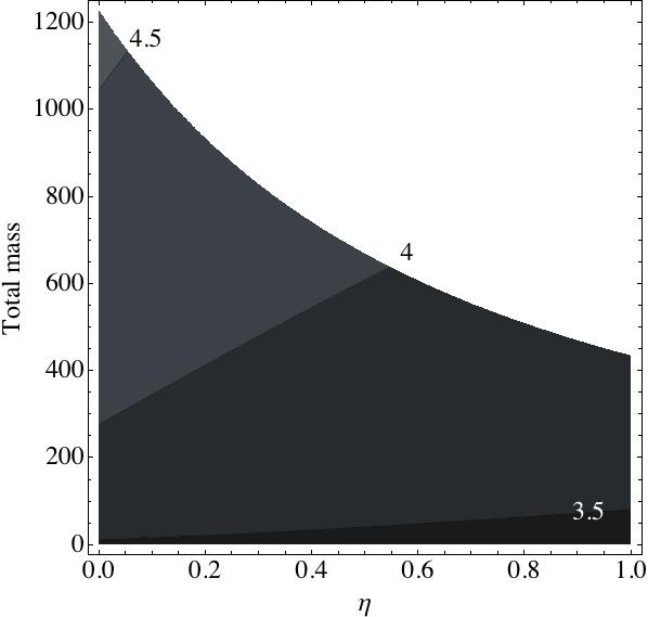
(a)  $\delta=0.1$

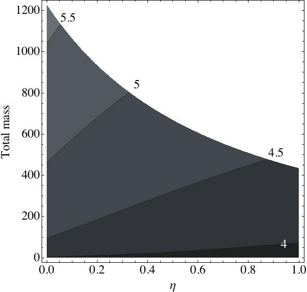
(b)  $\delta=0.05$

(c)  $\delta=0.01$

Figure 1: Contour plots showing the post-Newtonian orders $q/2$ needed to estimate $R_{cyc}^{(q)}$ with a precision (relative to the 2.5PN contribution) of 1(a) $10\%$, 1(b) $5\%$, and 1(c) $1\%$ as a function of the total mass (in $M_{\odot}$) and the mass ratio $\eta$. The white areas indicate those binaries with masses that have ISCO frequencies lower than $10$Hz, which we regard here as not detectable by LIGO.

The $p,q=0$ term in (78) denotes the leading order (i.e., Newtonian) prediction for $N_{cyc}$ and is often used for making rough estimates of the number of cycles spent in LIGO’s bandwidth. The remaining terms are the post-Newtonian corrections from higher order gravitational, relativistic, spin, radiation reaction, and finite size effects. If we regard LIGO’s lowest detectable frequency to be approximately 10 Hz then the ratio

$$R_{cyc}^{(q)}(10{\rm\,Hz})\equiv\frac{N_{cyc}^{(p,q)}(10{\rm\,Hz})}{N_{cyc}^{(p,5)}(10{\rm\,Hz})}\approx\frac{3\xi^{(q-5)/3}}{q-5}\frac{f_{isco}^{(q-5)/3}-10^{(q-5)/3}}{\ln(f_{isco}/10)},$$ (80)

with $q>5$ and $c_{pq}=O(1)$, gives an approximate measure of the corrections to the $O(1)$ number of cycles (i.e., the 2.5PN correction) from higher PN terms. Note that the ratio is independent of $p$.

From (80) we can estimate the approximate PN order, with a specified precision, that (78) should be expanded through. If $\delta$ denotes this precision then the PN order is approximately given by the solution of

$$R_{cyc}^{(q)}(10{\rm\,Hz})=\delta$$ (81)

for $q/2$. A more accurate treatment should be given by more quantitative means Thorne:RevModPhys52 ; Cutler:PRL70 but since $N_{cyc}$ is currently known only through 3.5PN Blanchet:LRR ; Maggiore then we will continue with this somewhat crude estimation.

Figures 1(a)-1(c) show contour plots of the solutions to (81) as a function of the binary’s total mass and the mass ratio for $\delta=0.1,0.05$, and $0.01$, respectively. For a precision of $\approx 10\%$ Figure 1(a) indicates that 3.5PN expressions are adequate for equal mass binaries with a total mass as high as $\sim 80M_{\odot}$ but that 4PN expressions may be more suitable for total masses between $\sim 80M_{\odot}-430M_{\odot}$. Equal mass binaries with a total mass $\mathrel{\hbox to0.0pt{\lower 3.0pt\hbox{\hskip 1.0pt$\sim$}\hss}\raise 1.0pt\hbox{$>$}}430M_{\odot}$ emit gravitational waves at the ISCO with frequencies less than 10Hz and therefore do not enter LIGO’s bandwidth. At a precision of $1\%$ Figure 1(c) shows that for a binary with a mass ratio of $1/10$ and a total mass of $1000M_{\odot}$ that one may need PN expressions to order 6.5PN. For a precision of $10\%$ Figure 1(a) implies that the same system may require 4.5PN corrections. Such high PN orders for this particular binary should be expected since its waveform is in LIGO’s observable bandwidth for a short frequency interval.

The plots in Figure (1) should be regarded as providing crude estimates for determining the PN orders needed for LIGO to measure the number of cycles in its bandwidth with a given precision. Of course, these estimates can be justified only after the PN expansion of $N_{cyc}$ has been performed to higher orders in conjunction with a more comprehensive analysis. Nevertheless, we believe that Figure (1) and the considerations of this section can serve as a motivation for calculating higher order corrections in the PN expansion for binaries with unequal masses.

IV Further developments

IV.1 Gravitational perturbation theory with self-consistent backreaction

The GP-SCB approach provides a general framework to build perturbation theories that are specific to the assumptions and input being considered. We demonstrated in Section II.2 how the well-known post-Newtonian expansion and perturbation theory for EMRIs can be derived in the GP-SCB formalism.

In Section II.3 we used the GP-SCB approach to introduce an adiabatic expansion with backreaction for arbitrary masses and velocities. Perhaps the most pertinent issue is determining the domain of validity of the equations of motion (57)-(62). In particular, the degree of accuracy of those equations needs to be determined by the data analysis requirements set by gravitational wave interferometers. Can these system of equations adequately capture the plunge and possibly merger phases? How does the mass ratio and relative velocity affect the answer to these questions, if at all? We hope to address these questions in some more detail in future papers GalleyHu:SCB1 ; GalleyHu:SCB2 .

A related issue is obtaining the solutions to such complicated backreaction equations. Since all of the degrees of freedom in the example of Section II.3 are interacting non-trivially and non-linearly with other variables it would seem that there is a rich variety of processes that makes calculating the number of cycles that a binary stays in a detector’s bandwidth, for example, difficult to perform and subsequently to compare with known results, both analytical and numerical. Furthermore, in many cases there are isometries associated with the background geometry that can be exploited to assist in developing (semi-)analytical solutions. This is the case with the post-Newtonian method applied to the Minkowski spacetime, which is maximally symmetric, and with EMRI-perturbation theories off a Kerr background, which is axisymmetric. However, there does not seem to be any isometry associated with the background metric $g_{0\mu\nu}$ since its evolution is determined in part by sources lacking any specific symmetry; see (57). Consequently, we will likely be forced to introduce some additional assumptions, but hopefully not as drastic as weak field, slow motion or small mass ratio, that could make it easier to find solutions beyond these simpler and more accessible regimes and provide new insights into processes hitherto too difficult to comprehend analytically.

There have been several approaches that are based on an adiabatic approximation from a two-time scale separation for EMRI binaries HindererFlanagan:PRD78 ; Mino:ProgTheorPhys113 ; Mino:ProgTheorPhys115 ; Mino:CQG22_1 ; Mino:CQG22_2 ; PoundPoisson:PRD77 . While our method is not restricted to extreme mass ratios, it is nevertheless more involved because the background geometry evolves with the backreaction from both the stress energy of the compact object (with finite size effects due to the extended nature of the mass) and the effective stress energy of the gravitational waves.

The generic framework for building perturbative expansions, originally developed in Anderson:PRD55 , may be useful for generating other approximations in addition to the one discussed in Section II.3. Depending on the dynamical regime of the two-body dynamics it may be possible to develop more perturbation theories suitable for other scenarios involving gravitational binaries including the head-on collision of two black holes, the merger of comparable mass compact objects, etc. One obvious perturbation theory that can be constructed would use the effective point particle description for both masses of the binary and derive the equations of motion in a similar manner as in Section II.3. Such a theory might lend itself useful to more practical schemes for solving the backreaction equations. We plan to investigate these and other issues associated with the self-consistent approach in future papers GalleyHu:SCB1 ; GalleyHu:SCB2 .

IV.2 Post-Newtonian effective field theory for arbitrary mass ratios

In Section III we provided crude estimates indicating the PN order that the number of gravitational wave cycles falling into LIGO’s bandwidth should be calculated through for several given precisions. The PN order depends non-trivially on the binary’s mass ratio and total mass. For a binary composed of $10M_{\odot}$ and $100M_{\odot}$ compact objects, Figure 1(b) suggests that one may need to calculate $N_{cyc}$ to 4.5PN to achieve a $\sim 5\%$ precision relative to the 2.5PN correction. We also find that for a constant total mass the PN order increases as the mass ratio decreases. Meanwhile, for a constant mass ratio the PN order increases as the total mass increases. Both results are expected on intuitive grounds.

Justifying these estimates requires computing to higher PN orders beyond the current 3.5PN expressions. In the PN-EFT approach, such calculations can be accomplished systematically and relatively efficiently compared to standard formalisms. Indeed, where higher PN orders are needed new physical interactions can manifest, including finite size effects from companion-induced tidal deformations (i.e., the non-effacement of internal structure), spin effects with radiation reaction, etc. We intend to investigate some of these features in future work.

- (1) A. Abramovici et al., Science 256, 325 (1992), http://www.ligo.caltech.edu.
- (2) The LISA website is http://lisa.nasa.gov.
- (3) T. Damour, 300 Years of Gravitation (Cambridge University Press, Cambridge, 1987), .
- (4) K. S. Thorne, Rev. Mod. Phys. 52, 299 (1980).
- (5) L. Blanchet, Living Reviews in Relativity 9 (2006).
- (6) Y. I. Toshifumi Futamase, Living Reviews in Relativity 10 (2007).
- (7) M. Maggiore, Gravitational Waves Volume 1: Theory and Experiments (Oxford University Press, Oxford, 2008).
- (8) W. Goldberger and I. Rothstein, Phys. Rev. D 73, 104029 (2006), hep-th/0409156.
- (9) G. ’t Hooft and M. Veltman, Nucl. Phys. B44, 189 (1972).
- (10) A. Buonanno and T. Damour, Phys. Rev. D 59, 084006 (1999), gr-qc/9811091.
- (11) A. Buonanno and T. Damour, Phys. Rev. D 62, 064015 (2000), [arXiv: gr-qc/0001013].
- (12) M. Boyle et al., Phys. Rev. D 78, 104020 (2008), [arXiv: 0804.4184].
- (13) T. Damour and A. Nagar, (2009), [arXiv: 0902.0136].
- (14) A. Buonanno et al., [arXiv: 0902.0790].
- (15) E. Poisson, Living Reviews in Relativity 7 (2004).
- (16) L. M. Burko, Phys. Rev. D 67, 084001 (2003), gr-qc/0208034.
- (17) J. Frank and M. J. Rees, Mon. Not. R. Astron. Soc. 176, 633 (1976).
- (18) T. A. Boroson and T. R. Lauer, Nature 458, 53 (2009).
- (19) C. M. Gaskell, (2009), [arXiv: 0903.4447].
- (20) P. R. Anderson, Phys. Rev. D 55, 3440 (1997).
- (21) P. R. Anderson, Phys. Rev. D 56, 4824 (1997).
- (22) C. R. Galley and B. L. Hu, New analytical methods for gravitational binary IMRI processes I. Perturbation theory with self-consistent backreaction (in preparation).
- (23) C. R. Galley and B. L. Hu, New analytical methods for gravitational binary IMRI processes II. Post-Newtonian effective field theory for arbitrary mass ratios (in preparation).
- (24) D. R. Brill and J. B. Hartle, Phys. Rev. 135, B271 (1964).
- (25) R. A. Isaacson, Phys. Rev. 166, 1263 (1968).
- (26) R. A. Isaacson, Phys. Rev. 166, 1272 (1968).
- (27) Y. Mino, M. Sasaki, and T. Tanaka, Phys. Rev. D 55, 3457 (1997), gr-qc/9606018.
- (28) T. C. Quinn and R. M. Wald, Phys. Rev. D 56, 3381 (1997), gr-qc/9610053.
- (29) C. R. Galley and B. L. Hu, Phys. Rev. D 79, 064002 (2009).
- (30) F. J. Zerilli, Phys. Rev. D 2, 2141 (1970).
- (31) L. S. Finn, Phys. Rev. D 46, 5236 (1992).
- (32) L. S. Finn and D. F. Chernoff, Phys. Rev. D 47, 2198 (1993).
- (33) C. Cutler et al., Phys. Rev. Lett. 70, 2984 (1993), astro-ph/9208005.
- (34) T. Hinderer and E. E. Flanagan, Phys. Rev. D 78, 064028 (2008).
- (35) Y. Mino, Prog. Theor. Phys. 113, 733 (2005).
- (36) Y. Mino, Prog. Theor. Phys. 115, 43 (2006).
- (37) Y. Mino, Class. Quantum Grav. 22, S375 (2007).
- (38) Y. Mino, Class. Quantum Grav. 22, S717 (2007).
- (39) A. Pound and E. Poisson, Phys. Rev. D 77, 044012 (2008).
- (40) M. E. Luke, A. V. Manohar, and I. Z. Rothstein, Phys. Rev. D 61, 074025 (2000).