The explicit expression of the fugacity for weakly interacting Bose and Fermi gases

Abstract

In this paper, we calculate the explicit expression for the fugacity for two- and three-dimensional weakly interacting Bose and Fermi gases from their equations of state in isochoric and isobaric processes, respectively, based on the mathematical result of the boundary problem of analytic functions — the homogeneous Riemann-Hilbert problem. We also discuss the Bose-Einstein condensation phase transition of three-dimensional hard-sphere Bose gases.

I Introduction

The physical problem. The equation of state for a quantum gas can be obtained by eliminating the fugacity $z$ between the equations

$$\frac{P}{kT} =\frac{1}{V}\ln\Xi\left(T,z,V\right),$$ (1)

$$n =\frac{1}{V}z\frac{\partial}{\partial z}\ln\Xi\left(T,z,V\right),$$ (2)

where $P$ is the pressure, $\ln\Xi$ the grand potential, $n$ the particle number density, and $V$ the volume. Concretely, for example, in isochoric processes, solving $z=z\left(n,T\right)$ from Eq. (2) and substituting it into Eq. (1) give the equation of state

$$\frac{P}{kT}=\left.\frac{1}{V}\ln\Xi\left(T,z,V\right)\right|_{z=z\left(n,T\right)},$$ (3)

and in isobaric processes, solving $z=z\left(P,T\right)$ from Eq. (1) and substituting it into Eq. (2) give the equation of state

$$n=\left.\frac{1}{V}z\frac{\partial}{\partial z}\ln\Xi\left(T,z,V\right)\right|_{z=z\left(P,T\right)}.$$ (4)

In a word, to solve, e.g., the pressure $P$ requires to solve the fugacity $z$ first. However, only in some simple cases, such as classical ideal gases Kadanoff , two-dimensional ideal quantum gases, the explicit expression of the fugacity $z$ can be obtained by solving Eq. (2) or (1). In most cases, the fugacity can only be obtained approximately, e.g., at high-temperature and low-density or low-temperature and high-density limit. In this paper, we will calculate the explicit expression for the fugacity for two- and three-dimensional weakly interacting hard-sphere Bose and Fermi gases by directly solving Eqs. (2) and (1) for isochoric and isobaric processes, respectively.

The hard-sphere gas, as a simplified model, is of great value for investigating the more general theory of interacting gases and can be extended to some more general cases. This is because a particle that is spread out in space sees only an averaged effect of the potential and, thus, often a complete knowledge of the detailed interaction potential is not necessary for a satisfactory description HYL ; HYL2 . Or, from the viewpoint of quantum mechanics, due to the low collision energy of collisions among the gas molecules, the shape-independent $s$-wave contribution dominates. The equations of state for three-dimensional hard-sphere Bose and Fermi gases are presented in Ref. LeeYang by the binary collision expansion method. The equations of state for two-dimensional cases is discussed in Ref. OurEPL . For one-dimensional cases, there are deeply analyses in Ref. Yang ; Yang2 ; Yang3 ; Yang4 ; Yang5 ; Yang6 ; Yang7 ; Yang8 ; Yang9 . Non-ideal quantum gases are studied from various aspects, e.g., equivalence between hard-sphere and zero-range potentials Val , thermodynamics RD ; HLD , ferromagnetic transitions SMB ; HH , and the upper limit on $T_{c}$ of BEC OurAnn . The second and third virial coefficients for strongly correlated fermions are discussed for two- LHD10 and three-dimensional LHD09 cases by using the few-particle exact solutions. Many methods are employed, e.g., auxiliary field MDC and cluster expansion SKU methods.

The mathematical method. The key idea of the method for solving the explicit expression for the fugacity from Eqs. (2) and (1) is based on the boundary problem of analytic functions — the homogeneous Riemann-Hilbert problem Muskhelishvili . In a Riemann-Hilbert problem, one seeks to find a sectionally analytic function $\psi\left(\zeta\right)$ under the boundary condition

$$\psi^{+}\left(\zeta\right)=G\left(\zeta\right)\psi^{-}\left(\zeta\right)+g\left(\zeta\right),\,\,\zeta\in L,$$ (5)

where $L$ is a union of a finite number of smooth simple arcs, $\psi^{+}\left(\zeta\right)$ and $\psi^{-}\left(\zeta\right)$ are boundary values of $\psi\left(\zeta\right)$ on the left and right of $L$, $G\left(\zeta\right)$ and $g\left(\zeta\right)$ are functions satisfying $\left|f\left(\zeta_{2}\right)-f\left(\zeta_{1}\right)\right|\leq A\left|\zeta_{2}-\zeta_{1}\right|^{\mu}$ with $A$, $\mu>0$, the Hölder condition, and $G\left(\zeta\right)\neq 0$ everywhere on $L$. The function $\psi\left(\zeta\right)$ being a sectionally analytic function means that $\psi\left(\zeta\right)$ is analytic in each region not containing points of the boundary $L$ and is continuous on $L$ from the left and from the right, excepting possibly some ends of $L$ and near such ends the function $\psi\left(\zeta\right)$ should satisfy

$$\left|\psi\left(\zeta\right)\right|<\frac{constant}{\left|\zeta-c_{k}\right|^{\alpha_{k}}},\,\,\,\alpha_{k}\,<1,$$ (6)

where $\alpha_{k}$ is a constant corresponding to the $k$-th end $c_{k}$. The homogeneous Riemann-Hilbert problem is a Riemann-Hilbert problem with $g\left(\zeta\right)=0$. In a homogeneous Riemann-Hilbert problem, the problem is converted into finding a function $\psi\left(\zeta\right)$ from the jump on the two sides of the boundary $L$, $G\left(\zeta\right)=\psi^{+}\left(\zeta\right)/\psi^{-}\left(\zeta\right)\,$.

Take an isochoric process as an example. In this case, the fugacity is determined by Eq. (2). The first step is to introduce a real function whose zero gives Eq. (2). Analytically continuing this real function to the complex plane gives a complex function, and, clearly, the zero of the real function becomes the zero of this complex function on the real axis. Therefore, the fugacity $z$ becomes a real zero of this complex function, and the problem of solving the fugacity is converted into a problem of seeking the real zero of such a complex function. The key step toward solving the zero relies on the homogeneous Riemann-Hilbert problem.

Based on the Riemann-Hilbert problem, Leonard calculates the explicit expression for the fugacity for ideal Bose and Fermi gases Leonard . We also construct an exactly solvable phase transition model, the generalized Bose–Einstein condensation, with the help of the Riemann-Hilbert problem Ours1 .

Note that besides Bose and Fermi cases, this method can also be used to solve the fugacity for intermediate statistics which describes various elementary excitations OurAnn2 ; OurJSP corresponding to various quantization schemes OurAnn3 . Moreover, the method can be applied to solve the ideal and interacting gases in confined space JMP07 ; PLA ; PLA2 ; PLA3 ; PLA4 ; PLA5 ; PLA6 ; PLA7 ; PLA8 .

Moreover, if a singularity appears in the relation of the fugacity $z$ and the temperature $T$, there is a phase transition. In this paper, we give rigorous results of the relation between $z$ and $T$, so we can judge the occurrence of a phase transition by observing the relation of $z$ and $T$ directly.

A detailed description of the method is given in Sec. II. In Secs. III and IV, we calculate the explicit expression for the fugacity for two- and three-dimensional hard-sphere Bose and Fermi gases, isochoric cases in Sec. III and isobaric cases in Sec. IV. In Sec. V, we compare our result with the virial expansion at high temperatures and low densities. In Sec. VI, we discuss the Bose-Einstein condensation phase transition of three–dimensional hard-sphere Bose gases. The conclusions are summarized in Sec. VII.

II The method

In this section, we give a description of the method.

II.1 The formal explicit expression of the fugacity

Take an isochoric process as an example for describing the method.

In an isochoric case, what we want to do is to solve an explicit expression for the fugacity $z$ from Eq. (2). Introduce a real function

$$\Psi\left(z\right)=\frac{1}{nV}z\frac{\partial}{\partial z}\ln\Xi\left(T,z,V\right)-1\equiv f\left(z\right)-1,$$ (7)

where $f\left(z\right)=\left(1/nV\right)z\left(\partial/\partial z\right)\ln\Xi\left(T,z,V\right)$. Clearly, Eq. (2) corresponds to $\Psi\left(z\right)=0$. In other words, the fugacity $z$ is a zero of the function $\Psi\left(z\right)$, and the problem of solving the fugacity $z$ is converted into the problem of seeking the zero of $\Psi\left(z\right)$.

To seek the zero of $\Psi\left(z\right)$, we first analytically continue the function $\Psi\left(z\right)$ to the whole complex $\zeta$-plane. The analytically continued function is

$$\Psi\left(\zeta\right)=f\left(\zeta\right)-1,\,\,\zeta\in\mathbb{C}.$$ (8)

The fugacity $z$ that we want to solve is a zero of the real function $\Psi\left(z\right)$ and is, of course, a zero of the complex function $\Psi\left(\zeta\right)$ on the real axis. Usually, the function $\Psi\left(\zeta\right)$ has not only one zero. Besides the zero corresponding to the fugacity $z$, there are still other zeros in the complex $\zeta$-plane, denoted as $\omega_{i}$, $\left(i=1,2,\cdots n_{\omega}-1\right)$, where $n_{\omega}$ is the total number of the zeros. Moreover, $\Psi\left(\zeta\right)$ may also has singularities in the complex $\zeta$-plane. In the following, we will show that in our case, $\Psi\left(\zeta\right)$ has no isolated singularities, and all its singularities are non-isolated singularities, forming some arcs in the complex $\zeta$-plane. Such arcs, which form a boundary of the analytic region of $\Psi\left(\zeta\right)$, will be denoted by $L_{i}$, $\left(i=1,2,\cdots,m_{L}\right)$, where $m_{L}$ is the total number of the arcs. That is to say, $\Psi\left(\zeta\right)$ is analytic in each region not containing points of the arcs $L_{i}$ and has $n_{\omega}$ zeros; at least one of the zeros of $\Psi\left(\zeta\right)$ is on the real axis. Therefore, we can express $\Psi\left(\zeta\right)$ in the following form:

$$\Psi\left(\zeta\right)=\eta\left(\zeta-z\right){\displaystyle\prod\limits_{i=1}^{n_{\omega}-1}}\left(\zeta-\omega_{i}\right)\Phi\left(\zeta\right),$$ (9)

where $\eta$ is a constant and $\Phi\left(\zeta\right)$ is a function vanishing nowhere in the complex $\zeta$-plane and analytic in each region not containing points of the arcs $L_{i}$. In principle, except the fugacity $z$, if we know all other $n_{\omega}-1$ zeros of $\Phi\left(\zeta\right)$, $\omega_{i}$, the explicit expression of $z$ can be formally expressed from Eq. (9),

$$z=\zeta-\left[\eta{\displaystyle\prod\limits_{i=1}^{n_{\omega}-1}}\left(\zeta-\omega_{i}\right)\right]^{-1}\frac{\Psi\left(\zeta\right)}{\Phi\left(\zeta\right)}.$$ (10)

Then, the problem of solving $z$ is converted into the problems of solving the function $\Phi\left(\zeta\right)$ and finding the zeros $\omega_{i}$.

II.2 $\Phi\left(\zeta\right)$ and the fundamental solution of the homogeneous Riemann-Hilbert problem

The function $\Phi\left(\zeta\right)$ can be determined with the help of the homogeneous Riemann-Hilbert problem.

In a homogeneous Riemann-Hilbert problem, if the jump of a function on the boundary is known, we can determine the function up to an arbitrary polynomial. To seek the function $\Phi\left(\zeta\right)$, we first need to solve the fundamental solution of the homogeneous Riemann-Hilbert problem, denoted as $\varphi\left(\zeta\right)$. The fundamental solution $\varphi\left(\zeta\right)$ is such a solution that $\varphi\left(\zeta\right)$ and its reciprocal $1/\varphi\left(\zeta\right)$ both are sectionally analytic functions. More concretely, a fundamental solution has no zeros and isolated singularities; all its singularities lie on some arcs, forming a boundary for the analytic region; at each end of the arcs, $c_{k}$, the degree of divergence of the solution $\varphi\left(\zeta\right)$ and its reciprocal $1/\varphi\left(\zeta\right)$ is less than $1$, i.e., $\left|\varphi\left(\zeta\right)\right|<constant/\left|\zeta-c_{k}\right|^{\alpha_{k}}$ and $\left|1/\varphi\left(\zeta\right)\right|<constant/\left|\zeta-c_{k}\right|^{\alpha_{k}^{\prime}}$, where $\alpha_{k}$ and $\alpha_{k}^{\prime}$ are constants less than $1$. The fundamental solution, generally speaking, is not completely determined by the above conditions; they are divided into some classes according to their behaviors near the ends, and any class of which can be chosen as the fundamental solution of the homogeneous Riemann-Hilbert problem. In this paper, we choose the fundamental solution satisfying

$$\left|\varphi\left(\zeta\right)\right|<\frac{constant}{\left|\zeta-c_{k}\right|^{\alpha_{k}}},\,\,\,0\leq\alpha_{k}\,<1.$$ (11)

Generally speaking, the function $\Phi\left(\zeta\right)$ that we want to find is not a fundamental solution though it has no zeros and isolated singularities and all its singularities lie on the arcs, $L_{i}$ ($i=1,\cdots,m_{L}$), since the degree of divergence of $\Phi\left(\zeta\right)$ or $1/\Phi\left(\zeta\right)$ at the ends of such arcs may not be less than $1$. However, in terms of the fundamental solution $\varphi\left(\zeta\right)$, the function $\Phi\left(\zeta\right)$ can always be expressed as

$$\Phi\left(\zeta\right)=\frac{\varphi\left(\zeta\right)}{{\displaystyle\prod\limits_{k=1}^{n}}\left(\zeta-c_{k}\right)^{\beta_{k}}},$$ (12)

where $n$ is the number of the ends that are different from infinity and $\beta_{k}$ is a constant determined by both the degree of divergence of $\Phi\left(\zeta\right)$ and the degree of divergence of the fundamental solution $\varphi\left(\zeta\right)$ at the $k$-th end $c_{k}$. For a chosen fundamental solution $\varphi\left(\zeta\right)$ (in the present case, the fundamental solution is chosen to satisfy Eq. (11)), $\beta_{k}$ should ensure that the behaviors of the two sides of Eq. (12) in the neighborhood of the $k$-th end of the arcs $L_{i}$ are the same. For the end at infinity, we need not pay special attention since at such an end the degree of divergence of the function encountered in the present case is less than $1$. Concretely, near infinity, the behavior of the function $\Psi\left(\zeta\right)$, defined by Eq. (8), lies on the asymptotic behavior of the Bose-Einstein integral or the Fermi-Dirac integral near infinity. Near the point of $\infty$, the Cauchy principal value of the analytically continued Bose-Einstein integral $g_{\sigma}\left(\zeta\right)\sim-\left(\ln\zeta\right)^{\sigma}/\left[\sigma\Gamma\left(\sigma\right)\right]$ Clunie , and then $\left.\Psi\left(\zeta\right)\right|_{\zeta\rightarrow\infty}\sim\left(\ln\zeta\right)^{k}$, where $k$ is a constant; near the point of $-\infty$, the Cauchy principal value of the analytically continued Fermi-Dirac integral $f_{\sigma}\left(\zeta\right)\sim\left[\ln\left(-\zeta\right)\right]^{\sigma}/\left[\sigma\Gamma\left(\sigma\right)\right]$, and then $\left.\Psi\left(\zeta\right)\right|_{\zeta\rightarrow-\infty}\sim\left[\ln\left(-\zeta\right)\right]^{k}$.

The fundamental solution $\varphi\left(\zeta\right)$ can be obtained based on the result of the homogeneous Riemann-Hilbert problem. From Eqs. (9) and (12), we can see that the jumps of the functions $\Psi\left(\zeta\right)$, $\Phi\left(\zeta\right)$, and $\varphi\left(\zeta\right)$ at the two sides of the boundary, which consists of arcs $L_{i}$, are the same, i.e.,

$$\frac{\varphi^{+}\left(\zeta\right)}{\varphi^{-}\left(\zeta\right)}=\frac{\Phi^{+}\left(\zeta\right)}{\Phi^{-}\left(\zeta\right)}=\frac{\Psi^{+}\left(\zeta\right)}{\Psi^{-}\left(\zeta\right)}\equiv G\left(\zeta\right),\text{ }\zeta\in L_{i},(i=1,2,\cdots m_{L}).$$ (13)

According to the homogeneous Riemann-Hilbert problem, from the jump $G\left(\zeta\right)$, the fundamental solution $\varphi\left(\zeta\right)$ can be determined:

$$\varphi\left(\zeta\right)=e^{\gamma\left(\zeta\right)}{\displaystyle\prod\limits_{k=1}^{n}}\left(\zeta-c_{k}\right)^{\lambda_{k}},$$ (14)

where

$$\gamma\left(\zeta\right)=\frac{1}{2\pi i}\int\limits_{L_{1}+L_{2}+\cdots+L_{m_{L}}}d\xi\frac{\ln G\left(\xi\right)}{\xi-\zeta},$$ (15)

and the integral is along the boundary, consisting of the arcs $L_{1}$, $L_{2}$, $\cdots$, and $L_{m_{L}}$. The parameter $\lambda_{k}$ in Eq. (14) is an integer determined by the following conditions:

$$\mp\operatorname{Re}\frac{\ln G\left(c_{k}\right)}{2\pi i}+\lambda_{k} =0,\text{\thinspace\thinspace\thinspace\thinspace\thinspace if\ }\mp\operatorname{Re}\frac{\ln G\left(c_{k}\right)}{2\pi i}\text{\thinspace\thinspace is an integer,}$$ (16)

$$-1 <\mp\operatorname{Re}\frac{\ln G\left(c_{k}\right)}{2\pi i}+\lambda_{k}<1,\text{\thinspace\thinspace\thinspace other cases,}$$ (17)

where the upper sign ”$-$” has to be taken for the starting point of a certain arc, $L_{i}$, the lower ”$+$” for the end point. The condition (17) becomes

$$-1<\mp\operatorname{Re}\frac{\ln G\left(c_{k}\right)}{2\pi i}+\lambda_{k}<0$$ (18)

when the fundamental solution is chosen to satisfy Eq. (11).

By Eq. (13), we can see that the jump $G\left(\zeta\right)$ of the fundamental solution $\varphi\left(\zeta\right)$ at the two sides of the boundary is equal to the jump of $\Psi\left(\zeta\right)$, a known function defined by Eqs. (7) and (8), along the boundary. This allows us to determine the jump $G\left(\zeta\right)$ by $\Psi\left(\zeta\right)$ and then to determine the fundamental solution $\varphi\left(\zeta\right)$ by $G\left(\zeta\right)$.

II.3 Zeros

The fugacity $z$ is one of the zeros of the function $\Psi\left(\zeta\right)$ on the real axis. In principle, after obtaining $\Psi\left(\zeta\right)$, except the zero $z$, if we know all other $n_{\omega}-1$ zeros $\omega_{i}$ of $\Psi\left(\zeta\right)$, we can write down the explicit expression for $z$ as in Eq. (10). However, the difficulty of finding the zeros $\omega_{i}$ is often the same as the difficulty of finding the zero $z$. That is to say, it is actually impossible to solve $z$ by first solving the $n_{\omega}-1$ zeros $\omega_{i}$.

Alternatively, to find the zero $z$, we note that Eq. (9) is essentially an equation of $z$, $\omega_{i}$, and a parameter $\eta$. Based on Eq. (9), we have two possible ways to construct a set of equations for $z$, $\omega_{i}$, and $\eta$:

(1) Different values of $\zeta$ give different equations of $z$, $\omega_{i}$, and $\eta$, and $n_{\omega}+1$ different $\zeta$’s give a set of $n_{\omega}+1$ equations. Then, solving such a set of equations gives the fugacity $z$.

(2) Deriving both sides of Eq. (9) $\nu$ times ($\nu=0,1,2,\ldots,n_{\omega}$) and using Eq. (12) give $n_{\omega}+1$ equations of $z$, $\omega_{i}$, and $\eta$,

$$\left.{\displaystyle\prod\limits_{k=1}^{n}}\left(\zeta-c_{k}\right)^{\beta_{k}}\frac{\Psi\left(\zeta\right)}{\varphi\left(\zeta\right)}\right|_{\zeta=\zeta_{0}} =\left.\eta\left(\zeta-z\right){\displaystyle\prod\limits_{i=1}^{n_{\omega}-1}}\left(\zeta-\omega_{i}\right)\right|_{\zeta=\zeta_{0}},$$

$$\frac{d}{d\zeta}\left[{\displaystyle\prod\limits_{k=1}^{n}}\left(\zeta-c_{k}\right)^{\beta_{k}}\frac{\Psi\left(\zeta\right)}{\varphi\left(\zeta\right)}\right]_{\zeta=\zeta_{1}} =\frac{d}{d\zeta}\left[\eta\left(\zeta-z\right){\displaystyle\prod\limits_{i=1}^{n_{\omega}-1}}\left(\zeta-\omega_{i}\right)\right]_{\zeta=\zeta_{1}},$$

$$\cdots\cdots$$

$$\frac{d^{n_{\omega}}}{d\zeta^{n_{\omega}}}\left[{\displaystyle\prod\limits_{k=1}^{n}}\left(\zeta-c_{k}\right)^{\beta_{k}}\frac{\Psi\left(\zeta\right)}{\varphi\left(\zeta\right)}\right]_{\zeta=\zeta_{n_{\omega}}} =\frac{d^{n_{\omega}}}{d\zeta^{n_{\omega}}}\left[\eta\left(\zeta-z\right){\displaystyle\prod\limits_{i=1}^{n_{\omega}-1}}\left(\zeta-\omega_{i}\right)\right]_{\zeta=\zeta_{n_{\omega}}}.$$ (19)

In our case, it is convenient to chose $\zeta_{0}=\zeta_{1}=\cdots=\zeta_{n_{\omega}}=0$.

In the following, we will construct the equations for zeros by the second approach.

To find the zeros, we need to construct a set of $n_{\omega}+1$ equations. To achieve this, we need first to know the value of $n_{\omega}$, the number of zeros of $\Psi\left(\zeta\right)$. In our case, as the function $\Psi\left(\zeta\right)$ has no singularities besides the singularities on the boundary, the number of the zeros $n_{\omega}$ can be determined with the help of the argument principle: Along a contour surrounding the complex plane except the boundary, the change of the argument of $\Psi\left(\zeta\right)$ is proportional to the number of zeros.

III The explicit expression for the fugacity: isochoric processes

In this section, we will solve the explicit expression for the fugacity for weakly interacting Bose and Fermi gases from their equations of state directly by the method described above. For the weakly interacting case, the contribution of the collision between gas molecules mainly comes from the $s$-wave contribution, so the weakly interacting gas can be regarded as a hard-sphere gas consisting of hard-sphere particles with the scattering length as its diameter. In the case of Bose gases, we will not consider the problem of phase transition. It should be noted here that since the equation of state given by Lee and Yang LeeYang is an approximate result for weakly interacting hard-sphere gases, the expression of the fugacity is, though explicit, an approximate one limited by the approximation of the equation of state.

III.1 Three-dimensional hard-sphere Bose gases

The equation of state for three-dimensional weakly interacting hard-sphere Bose gases, up to first order of $a/\lambda$, is LeeYang

$$\frac{P}{kT} =\frac{1}{V}\ln\Xi\left(T,z,V\right)=\left(2j+1\right)\frac{1}{\lambda^{3}}\left[g_{5/2}\left(z\right)-2\left(j+1\right)\frac{a}{\lambda}g_{3/2}^{2}\left(z\right)\right],$$ (20)

$$n =\frac{1}{V}z\frac{\partial}{\partial z}\ln\Xi\left(T,z,V\right)=\left(2j+1\right)\frac{1}{\lambda^{3}}\left[g_{3/2}\left(z\right)-4\left(j+1\right)\frac{a}{\lambda}g_{1/2}\left(z\right)g_{3/2}\left(z\right)\right],$$ (21)

where $a$ is the scattering length, $\lambda=h/\sqrt{2\pi mkT}$ the mean thermal wavelength, $j$ the spin of the particle, and

$$g_{\sigma}\left(z\right)=\frac{1}{\Gamma(\sigma)}\int_{0}^{\infty}\frac{t^{\sigma-1}}{z^{-1}e^{t}-1}dt$$ (22)

the Bose-Einstein integral.

In an isochoric process, the fugacity $z=z\left(n,T\right)$ can be solved from Eq. (21). That is to say, as discussed in the above section, the fugacity $z$ is a zero of the real function $\Psi_{1}\left(z\right)=\left(1/nV\right)z\left(\partial/\partial z\right)\ln\Xi-1$. Analytically continuing $\Psi_{1}\left(z\right)$ to the entire complex plane gives

$$\Psi_{1}\left(\zeta\right)=\left(2j+1\right)\frac{1}{n\lambda^{3}}\left[g_{3/2}\left(\zeta\right)-4\left(j+1\right)\frac{a}{\lambda}g_{1/2}\left(\zeta\right)g_{3/2}\left(\zeta\right)\right]-1,$$ (23)

where $g_{\sigma}\left(\zeta\right)$ is an analytic continuation of the Bose-Einstein integral $g_{\sigma}\left(z\right)$. Generally speaking, $\Psi_{1}\left(\zeta\right)$ has more than one zero in the complex $\zeta$-plane, and the fugacity is one of these zeros on the real axis.

By expressing $\Psi_{1}\left(\zeta\right)$ as

$$\Psi_{1}\left(\zeta\right)=\eta_{1}\left(\zeta-z\right){\displaystyle\prod\limits_{i=1}^{n_{\omega}-1}}\left(\zeta-\omega_{i}\right)\Phi_{1}\left(\zeta\right),$$ (24)

where $z$ is the zero corresponding to the fugacity, $\omega_{i}$ ($i=1,\cdots,n_{\omega}-1$) are other zeros of $\Psi_{1}\left(\zeta\right)$ besides $z$, and $\eta_{1}$ is a constant, we define a function $\Phi_{1}\left(\zeta\right)$ with no zeros. To determine $\Phi_{1}\left(\zeta\right)$, we need to analyze the behavior of the singularity of $\Psi_{1}\left(\zeta\right)$ in the $\zeta$-plane. From Eq. (23), we can see that the singularity of $\Psi_{1}\left(\zeta\right)$ is determined by the singularity of the analytically continued Bose-Einstein integrals $g_{1/2}\left(\zeta\right)$ and $g_{3/2}\left(\zeta\right)$. The analytically continued Bose-Einstein integral $g_{\sigma}\left(\zeta\right)$ is just the polylogarithm function, or the Jonquiére function, $Li_{\sigma}\left(\zeta\right)$, a special case of the Lerch function, which is analytic in the region with the boundary along the positive real axis from $1$ to $\infty$ MOS . In other words, the analytically continued Bose-Einstein integral $g_{\sigma}\left(\zeta\right)$ has no isolated singularities, and all the singularities lie on the line from $1$ to $\infty$ on the real axis, i.e., the boundary is $\left[1,\infty\right)$. Consequently, according to Eqs. (23) and (24), $\Psi_{1}\left(\zeta\right)$ and $\Phi_{1}\left(\zeta\right)$ also have no isolated singularities, and all their singularities lie on the line $L$ from $1$ to $\infty$ on the real axis, i.e., in this case, the boundary of the analytic region consists of only one line. The function $\Phi_{1}\left(\zeta\right)$ is analytic in the region with the boundary $L$ and everywhere different from zero.

Calculating $\Phi_{1}\left(\zeta\right)$ needs the solution of the homogeneous Riemann-Hilbert problem. Eq. (12) gives the relation between $\Phi_{1}\left(\zeta\right)$ and the fundamental solution of the homogeneous Riemann-Hilbert problem $\varphi_{1}\left(\zeta\right)$. As we have chosen the fundamental solution satisfying Eq. (11), the parameter $\beta_{k}$ in Eq. (12) can be determined by the demand that the choice of $\beta_{k}$ must ensure that the behaviors of both sides of Eq. (12) are the same at each end. In our problem, the boundary of the analytic region of $\Psi_{1}\left(\zeta\right)$ has only one end $\zeta=1$ besides the end at infinity. Near the end $\zeta=1$,

$$\left.\Psi_{1}\left(\zeta\right)\right|_{\zeta\rightarrow 1}\sim\frac{1}{\sqrt{\zeta-1}},$$ (25)

i.e., $\Psi_{1}\left(\zeta\right)$ is divergent near $\zeta=1$ with a degree less than $1$. This means $\beta=0$. The singularities of $\Phi_{1}\left(\zeta\right)$ and $\Psi_{1}\left(\zeta\right)$ are the same, so $\Phi_{1}\left(\zeta\right)$ itself is just the fundamental solution, i.e., $\Phi_{1}\left(\zeta\right)=\varphi_{1}\left(\zeta\right)$.

To solve the fundamental solution $\varphi_{1}\left(\zeta\right)$, we first need to calculate the jump,

$$G_{1}\left(x\right)=\frac{\varphi_{1}^{+}\left(x\right)}{\varphi_{1}^{-}\left(x\right)}=\frac{\Psi_{1}^{+}\left(x\right)}{\Psi_{1}^{-}\left(x\right)},\text{ }x\in\left[1,\infty\right),$$ (26)

on the boundary, according to Eq. (13).

The jump of $\Psi_{1}\left(\zeta\right)$ on the boundary, according to Eq. (23), is determined by the jump of the analytically continued Bose-Einstein integral $g_{\sigma}\left(\zeta\right)$, the polylogarithm function $Li_{\sigma}\left(\zeta\right)$. The imaginary part of the polylogarithm function $Li_{\sigma}\left(\zeta\right)$ has a discontinuity on the boundary $\left[1,\infty\right)$ Wood :

$$\operatorname{Im}Li_{\sigma}\left(x\pm i\delta\right)=\pm\frac{\pi}{\Gamma\left(\sigma\right)}\left(\ln x\right)^{\sigma-1},\text{ }x\in\left[1,\infty\right),$$ (27)

where $\delta$ is a small positive quantity. Therefore, the values of the analytically continued Bose-Einstein integral at two sides of the boundary are

$$g_{\sigma}^{\pm}\left(x\right)=Li_{\sigma}^{\pm}\left(x\right)=\mathfrak{g}_{\sigma}\left(x\right)\pm i\frac{\pi}{\Gamma\left(\sigma\right)}\left(\ln x\right)^{\sigma-1},\text{ \ }x\in\left[1,\infty\right),$$ (28)

where

$$\mathfrak{g}_{\sigma}\left(x\right)\equiv\frac{1}{\Gamma(\sigma)}\mathbb{P}\int_{0}^{\infty}\frac{t^{\sigma-1}}{x^{-1}e^{t}-1}dt,\text{ }\sigma\neq 0$$ (29)

denotes the Cauchy principal value of the analytically continued Bose-Einstein integral $g_{\sigma}\left(\zeta\right)$ at the point $x$ on the boundary Clunie . Note that the Bose-Einstein integral $g_{0}\left(x\right)$, i.e., the case of $\sigma=0$, is an exception. $g_{0}\left(\zeta\right)=\zeta/\left(1-\zeta\right)$ has only one singularity $\zeta=1$, but has no singularities on the region $\left(1,\infty\right)$ on the real axis. Accordingly, by Eq. (23), the values of $\Psi_{1}\left(\zeta\right)$ on both sides of the boundary $\left[1,\infty\right)$ are

$$\Psi_{1}^{\pm}\left(x\right) =\left(2j+1\right)\frac{1}{n\lambda^{3}}\left\{\mathfrak{g}_{3/2}\left(x\right)-4\left(j+1\right)\frac{a}{\lambda}\left[\mathfrak{g}_{1/2}\left(x\right)\mathfrak{g}_{3/2}\left(x\right)-2\pi\right]\right\}-1$$

$$\pm i\left(2j+1\right)\frac{1}{n\lambda^{3}}2\sqrt{\pi}\sqrt{\ln x}\left\{1-2\left(j+1\right)\frac{a}{\lambda}\left[\frac{1}{\ln x}\mathfrak{g}_{3/2}\left(x\right)+2\mathfrak{g}_{1/2}\left(x\right)\right]\right\}.$$ (30)

Clearly, $\Psi_{1}^{+}\left(x\right)$ and $\Psi_{1}^{-}\left(x\right)$ are complex conjugate to each other, i.e., $\Psi_{1}^{+}\left(x\right)=\left[\Psi_{1}^{-}\left(x\right)\right]^{\ast}$, and the jump on the boundary $\left[1,\infty\right)$ is then

$$G_{1}\left(x\right)=\exp\left[i2\arg\Psi_{1}^{+}\left(x\right)\right],$$ (31)

where the argument of $\Psi_{1}^{+}\left(x\right)$ is

$$\arg\Psi_{1}^{+}\left(x\right)=\operatorname{arccot}\frac{\operatorname{Re}\Psi_{1}^{+}\left(x\right)}{\operatorname{Im}\Psi_{1}^{+}\left(x\right)}.$$ (32)

Now, the fundamental solution $\varphi_{1}\left(\zeta\right)$ can be solved by use of Eq. (14) directly. In our problem, the boundary has only one end different from infinity, $\zeta=1$, which means

$$\varphi_{1}\left(\zeta\right)=e^{\gamma_{1}\left(\zeta\right)}\left(\zeta-1\right)^{\lambda_{1}},$$ (33)

where

$$\gamma_{1}\left(\zeta\right)=\frac{1}{\pi}{\displaystyle\int\nolimits_{1}^{\infty}}dx\frac{\arg\Psi_{1}^{+}\left(x\right)}{x-\zeta}$$ (34)

and $\lambda_{1}$ is determined by Eq. (18). Choosing $\arg\Psi_{1}^{+}\left(\infty\right)=0$, we have $\arg\Psi_{1}^{+}\left(1\right)=-3\pi/2$. As the fundamental solution satisfies Eq. (11), the relation Eq. (18) becomes

$$-1<-\frac{1}{\pi}\arg\Psi_{1}^{+}\left(1\right)+\lambda_{1}<0,$$ (35)

and gives $\lambda_{1}=-2$. Therefore,

$$\Phi_{1}\left(\zeta\right)=\varphi_{1}\left(\zeta\right)=\frac{e^{\gamma_{1}\left(\zeta\right)}}{\left(\zeta-1\right)^{2}}.$$ (36)

By Eq. (24), we can construct a set of equations for zeros. For this purpose, we need to determine the number of the zeros of $\Psi_{1}\left(\zeta\right)$. The fact that the function $\Psi_{1}\left(\zeta\right)$ has no singularities besides the boundary $\left[1,\infty\right)$ allows us to use the argument principle to determine the number of its zeros in the complex $\zeta$-plane directly. Applying the argument principle along the contour surrounding the complex plane except the boundary $\left[1,\infty\right)$ shows that $\Psi_{1}\left(\zeta\right)$ has two zeros, denoted as $z$ (the fugacity) and $\omega$. Substituting Eq. (36) into Eq. (24) with $n_{\omega}=2$ gives

$$\Psi_{1}\left(\zeta\right)=\eta_{1}\frac{\left(\zeta-z\right)\left(\zeta-\omega\right)}{\left(\zeta-1\right)^{2}}e^{\gamma_{1}\left(\zeta\right)}.$$ (37)

From Eq. (37), we can construct a set of equations for $z$, $\omega$, and $\eta_{1}$. Since in this case, the values of the functions in Eq. (37) are relatively easy to be carried out at $\zeta=0$, we adopt the second method introduced in Sec. II.3: Derive both sides of Eq. (37) to construct various equations for zeros. In this case, we need three equations for determining $z$, $\omega$, and $\eta_{1}$. When $\zeta=0$, by Eq. (19), we have

$$\left\{\begin{array}[c]{l}\displaystyle\eta_{1}z\omega e^{\gamma_{1}\left(0\right)}=\Psi_{1}\left(0\right),\\ \displaystyle\eta_{1}z\omega e^{\gamma_{1}\left(0\right)}\left[\gamma_{1}^{\prime}\left(0\right)-\frac{1}{z}-\frac{1}{\omega}+2\right]=\Psi_{1}^{\prime}\left(0\right),\\ \displaystyle\eta_{1}z\omega e^{\gamma_{1}\left(0\right)}\left\{\gamma_{1}^{\prime}\left(0\right)^{2}-2\left[\gamma_{1}^{\prime}\left(0\right)+2\right]\left(\frac{1}{z}+\frac{1}{\omega}\right)+4\gamma_{1}^{\prime}\left(0\right)+\gamma_{1}^{\prime\prime}\left(0\right)+\frac{2}{z\omega}+6\right\}=\Psi_{1}^{\prime\prime}\left(0\right),\end{array}\right.$$ (38)

where

$$\gamma_{1}^{\left(n\right)}\left(0\right)=\frac{n!}{\pi}\int_{1}^{\infty}\frac{\arg\Psi_{1}^{+}\left(x\right)}{x^{n+1}}dx.$$ (39)

Consequently, the fugacity $z$ can be obtained by solving Eq. (38):

$$z =2\frac{n\lambda^{3}}{2j+1}\left\{1+\frac{n\lambda^{3}}{2j+1}\left[\gamma_{1}^{\prime}\left(0\right)+2\right]+\left\{1-2\frac{n\lambda^{3}}{2j+1}\left[\gamma_{1}^{\prime}\left(0\right)+2-\frac{\sqrt{2}}{2}+8\left(j+1\right)\frac{a}{\lambda}\right]\right.\right.$$

$$\left.\left.-\frac{\left(n\lambda^{3}\right)^{2}}{\left(2j+1\right)^{2}}\left[4\gamma_{1}^{\prime}\left(0\right)+\gamma_{1}^{\prime}\left(0\right)^{2}-2\gamma_{1}^{\prime\prime}\left(0\right)\right]\right\}^{1/2}\right\}^{-1}.$$ (40)

Substituting the fugacity $z$ given by Eq. (40) into Eq. (20) gives the equation of state. Note that the fugacity here is an explicit function of the temperature $T$.

To illustrate the above result more clearly, we plot the fugacity as a function of temperature in figure 1. Since eq. (40) is an exact solution of eq. (21), the result is exactly the same as the numerical solution of eq. (21). Note that at this situation, the fugacity has a maximum value, i.e., the curve in figure 1 has an end.

Figure 1: The relation between $z$ and $T$ for three-dimensional hard-sphere Bose gases in an isochoric process.

III.2 Three-dimensional hard-sphere Fermi gases

The equation of state for three-dimensional weakly interacting hard-sphere Fermi gases, up to first order of $a/\lambda$, is LeeYang

$$\frac{P}{kT} =\left(2j+1\right)\frac{1}{\lambda^{3}}\left[f_{5/2}\left(z\right)-2j\frac{a}{\lambda}f_{3/2}^{2}\left(z\right)\right],$$ (41)

$$n =\left(2j+1\right)\frac{1}{\lambda^{3}}\left[f_{3/2}\left(z\right)-4j\frac{a}{\lambda}f_{1/2}\left(z\right)f_{3/2}\left(z\right)\right],$$ (42)

where the Fermi-Dirac integral

$$f_{\sigma}\left(z\right)=\frac{1}{\Gamma(\sigma)}\int_{0}^{\infty}\frac{t^{\sigma-1}}{z^{-1}e^{t}+1}dt.$$ (43)

In an isochoric process, the fugacity $z=z\left(n,T\right)$ can be solved from Eq. (42). The fugacity $z$ is a zero of the complex function

$$\Psi_{2}\left(\zeta\right)=\left(2j+1\right)\frac{1}{n\lambda^{3}}\left[f_{3/2}\left(\zeta\right)-4j\frac{a}{\lambda}f_{1/2}\left(\zeta\right)f_{3/2}\left(\zeta\right)\right]-1$$ (44)

on the real axis, where $f_{\sigma}\left(\zeta\right)$ is the analytically continued Fermi-Dirac integral. The singularity of $\Psi_{2}\left(\zeta\right)$ is determined by the singularity of the analytically continued Fermi-Dirac integral. The analytically continued Fermi-Dirac integral here is the polylogarithm function $-Li_{\sigma}\left(-\zeta\right)$, which is analytic in the region with the boundary $\left[-1,-\infty\right)$.

By the argument principle, along the contour surrounding the complex plane except the boundary $\left[-1,-\infty\right)$, we can determine that $\Psi_{2}\left(\zeta\right)$ has two real zeros on the real axis; one of these two zeros is just the fugacity $z$. Accordingly, $\Psi_{2}\left(\zeta\right)$ can be expressed as

$$\Psi_{2}\left(\zeta\right)=\eta_{2}\left(\zeta-z\right)\left(\zeta-\omega\right)\Phi_{2}\left(\zeta\right),$$ (45)

where the function $\Phi_{2}\left(\zeta\right)$ has the same singularities as those of $\Psi_{2}\left(\zeta\right)$, lying on the line $\left[-1,-\infty\right)$, and has no zeros.

As stated above, in our case, the fundamental solution is chosen to satisfy Eq. (11). Near the end different from infinity of the boundary $\left[-1,-\infty\right)$, $\zeta=-1$, we have

$$\left.\Psi_{2}\left(\zeta\right)\right|_{\zeta\rightarrow-1}\sim\frac{1}{\sqrt{\zeta+1}}.$$ (46)

The degree of divergence of $\Psi_{2}\left(\zeta\right)$ at the end $\zeta=-1$ being less than $1$ implies that the function $\Phi_{2}\left(\zeta\right)$ itself is a fundamental solution of the homogeneous Riemann-Hilbert problem, i.e., $\Phi_{2}\left(\zeta\right)=\varphi_{2}\left(\zeta\right)$, where $\varphi_{2}\left(\zeta\right)$ denotes the fundamental solution.

To solve the fundamental solution $\varphi_{2}\left(\zeta\right)$, we need to know the jump on the boundary. From Eq. (13), we have

$$G_{2}\left(x\right)=\frac{\varphi_{2}^{+}\left(x\right)}{\varphi_{2}^{-}\left(x\right)}=\frac{\Psi_{2}^{+}\left(x\right)}{\Psi_{2}^{-}\left(x\right)},\text{ }x\in\left[-1,-\infty\right),$$ (47)

and from Eq. (27), we have

$$f_{\sigma}^{\pm}\left(x\right)=-Li_{\sigma}^{\pm}\left(-x\right)=\mathfrak{f}_{\sigma}\left(x\right)\mp i\frac{\pi}{\Gamma\left(\sigma\right)}\left[\ln\left(-x\right)\right]^{\sigma-1},$$ (48)

where

$$\mathfrak{f}_{\sigma}\left(x\right)=\frac{1}{\Gamma(\sigma)}\mathbb{P}\int_{0}^{\infty}\frac{t^{\sigma-1}}{x^{-1}e^{t}+1}dt,\text{ }\sigma\neq 0$$ (49)

is the Cauchy principal value of the analytically continued Fermi-Dirac integral. Notice that $x<0$. Then, the value of $\Psi_{2}\left(\zeta\right)$ at the two sides of the boundary can be obtained directly:

$$\Psi_{2}^{\pm}\left(x\right) =\left(2j+1\right)\frac{1}{n\lambda^{3}}\left\{\mathfrak{f}_{3/2}\left(x\right)-4j\frac{a}{\lambda}\left[\mathfrak{f}_{1/2}\left(x\right)\mathfrak{f}_{3/2}\left(x\right)-2\pi\right]\right\}-1$$

$$\mp i\left(2j+1\right)\frac{1}{n\lambda^{3}}2\sqrt{\pi}\sqrt{\ln\left(-x\right)}\left\{1-2j\frac{a}{\lambda}\left[\frac{1}{\ln\left(-x\right)}\mathfrak{f}_{3/2}\left(x\right)+2\mathfrak{f}_{1/2}\left(x\right)\right]\right\}.$$ (50)

$\Psi_{2}^{+}\left(x\right)$ and $\Psi_{2}^{-}\left(x\right)$ are complex conjugate to each other, so the jump of $\Psi_{2}\left(x\right)$ on the boundary $\left[-1,-\infty\right)$ is

$$G_{2}\left(x\right)=\exp\left[i2\arg\Psi_{2}^{+}\left(x\right)\right],$$ (51)

where the argument $\arg\Psi_{2}^{+}\left(x\right)=\operatorname{arccot}\left[\operatorname{Re}\Psi_{2}^{+}\left(x\right)/\operatorname{Im}\Psi_{2}^{+}\left(x\right)\right]$. Noting that in this case, there is only one end different from infinity of the boundary, $\zeta=-1$, we can write down the fundamental solution from Eq. (14):

$$\varphi_{2}\left(\zeta\right)=e^{\gamma_{2}\left(\zeta\right)}\left(\zeta+1\right)^{\lambda_{2}},$$ (52)

where

$$\gamma_{2}\left(\zeta\right)=\frac{1}{\pi}{\displaystyle\int\nolimits_{-1}^{-\infty}}dx\frac{\arg\Psi_{2}^{+}\left(x\right)}{x-\zeta}$$ (53)

and $\lambda_{2}$ will be determined by the condition (18). Choosing $\arg\Psi_{2}^{+}\left(-\infty\right)=0$ gives $\arg\Psi_{2}^{+}\left(-1\right)=-3\pi/2$. As the fundamental solution satisfies Eq. (11), the condition (18) becomes

$$-1<-\frac{1}{\pi}\arg\Psi_{2}^{+}\left(-1\right)+\lambda_{2}<0,$$ (54)

and gives $\lambda_{2}=-2$. Then,

$$\Phi_{2}\left(\zeta\right)=\varphi_{2}\left(\zeta\right)=\frac{e^{\gamma_{2}\left(\zeta\right)}}{\left(\zeta+1\right)^{2}}.$$ (55)

Substituting Eq. (55) into Eq. (45), we have

$$\Psi_{2}\left(\zeta\right)=\eta_{2}\frac{\left(\zeta-z\right)\left(\zeta-\omega\right)}{\left(\zeta+1\right)^{2}}e^{\gamma_{2}\left(\zeta\right)}.$$ (56)

To determine the zeros $z$, $\omega$ and the constant $\eta_{2}$, we need three equations. By setting $\zeta=0$, Eq. (56) and its first- and second-order derivatives give these three equations. Consequently, we have

$$z =2\frac{n\lambda^{3}}{2j+1}\left\{1+\frac{n\lambda^{3}}{2j+1}\left[\gamma_{2}^{\prime}\left(0\right)-2\right]+\left\{1-2\frac{n\lambda^{3}}{2j+1}\left[\gamma_{2}^{\prime}\left(0\right)-2+\frac{\sqrt{2}}{2}+8j\frac{a}{\lambda}\right]\right.\right.$$

$$\left.\left.+\frac{\left(n\lambda^{3}\right)^{2}}{\left(2j+1\right)^{2}}\left[4\gamma_{2}^{\prime}\left(0\right)-\gamma_{2}^{\prime}\left(0\right)^{2}+2\gamma_{2}^{\prime\prime}\left(0\right)\right]\right\}^{1/2}\right\}^{-1}.$$ (57)

This relation between $z$ and $T$ is plotted in figure 2.

Figure 2: The relation between $z$ and $T$ for three-dimensional hard-sphere Fermi gases in an isochoric process.

Substituting the fugacity $z$ given by Eq. (57) into Eq. (41) gives the equation of state.

III.3 Two-dimensional hard-sphere Bose gases

The equation of state for two-dimensional weakly interacting hard-sphere Bose gases, up to first order of $a/\lambda$, is OurEPL

$$\frac{P}{kT} =\left(2j+1\right)\frac{1}{\lambda^{2}}\left[g_{2}\left(z\right)-\left(j+1\right)\pi\frac{a}{\lambda}g_{1}\left(z\right)g_{3/2}\left(z\right)\right],$$ (58)

$$n =\left(2j+1\right)\frac{1}{\lambda^{2}}\left\{g_{1}\left(z\right)-\left(j+1\right)\pi\frac{a}{\lambda}\left[g_{0}\left(z\right)g_{3/2}\left(z\right)+g_{1/2}\left(z\right)g_{1}\left(z\right)\right]\right\},$$ (59)

where $n$ is the area density. In an isochoric process, the fugacity $z$ can be solved from Eq. (59). Following the above analysis, $z$ is a zero of the complex function

$$\Psi_{3}\left(\zeta\right)=\left(2j+1\right)\frac{1}{n\lambda^{2}}\left\{g_{1}\left(\zeta\right)-\left(j+1\right)\pi\frac{a}{\lambda}\left[g_{0}\left(\zeta\right)g_{3/2}\left(\zeta\right)+g_{1/2}\left(\zeta\right)g_{1}\left(\zeta\right)\right]\right\}-1$$ (60)

on the real axis. Note that $g_{\sigma}\left(\zeta\right)$ is an analytic continuation of the Bose-Einstein integral.

The singularities of $\Psi_{3}\left(\zeta\right)$ are determined by the singularities of the analytically continued Bose-Einstein integral $g_{\sigma}\left(\zeta\right)$, the polylogarithm function $Li_{\sigma}\left(\zeta\right)$. $\Psi_{3}\left(\zeta\right)$ has no isolated singularities, and all of its singularities form a line from $1$ to $\infty$ on the real axis. Similar to the three-dimensional case, by use of the argument principle, we can find that $\Psi_{3}\left(\zeta\right)$ has two zeros in the complex $\zeta$-plane, denoted as $z$ and $\omega$, where $z$ is the fugacity. As a result, $\Psi_{3}\left(\zeta\right)$ can be expressed as

$$\Psi_{3}\left(\zeta\right)=\eta_{3}\left(\zeta-z\right)\left(\zeta-\omega\right)\Phi_{3}\left(\zeta\right),$$ (61)

where the function $\Phi_{3}\left(\zeta\right)$ has no zeros, and its singularities also lie on the line $\left[1,\infty\right)$.

Near the end point $\zeta=1$ of the boundary of the analytic region of $\Psi_{3}\left(\zeta\right)$,

$$\left.\Psi_{3}\left(\zeta\right)\right|_{\zeta\rightarrow 1}\sim\frac{1}{\zeta-1},$$ (62)

i.e., $\Psi_{3}\left(\zeta\right)$ is linearly divergent near the point of $1$. As the singularities of $\Phi_{3}\left(\zeta\right)$ and $\Psi_{3}\left(\zeta\right)$ are the same, $\Phi_{3}\left(\zeta\right)$ is not a fundamental solution of the homogeneous Riemann-Hilbert problem. According to Eq. (12), we choose $\beta=1$ and express $\Phi_{3}\left(\zeta\right)$ as

$$\Phi_{3}\left(\zeta\right)=\frac{\varphi_{3}\left(\zeta\right)}{\zeta-1},$$ (63)

where $\varphi_{3}\left(\zeta\right)$ is a fundamental solution. To find the fundamental solution $\varphi_{3}\left(\zeta\right)$, we need the jump of $\Psi_{3}\left(\zeta\right)$ on the boundary $\left[1,\infty\right)$,

$$G_{3}\left(x\right)=\frac{\varphi_{3}^{+}\left(x\right)}{\varphi_{3}^{-}\left(x\right)}=\frac{\Psi_{3}^{+}\left(x\right)}{\Psi_{3}^{-}\left(x\right)},\text{ }x\in\left[1,\infty\right).$$ (64)

Similar to the three-dimensional case, the values of $\Psi_{3}\left(\zeta\right)$ at the two sides of the boundary $\left[1,\infty\right)$ are easy to be obtained from Eq. (60) by use of Eq. (28):

$$\Psi_{3}^{\pm}\left(x\right) =\left(2j+1\right)\frac{1}{n\lambda^{2}}\left\{\mathfrak{g}_{1}\left(x\right)-\left(j+1\right)\pi\frac{a}{\lambda}\left[g_{0}\left(x\right)\mathfrak{g}_{3/2}\left(x\right)+\mathfrak{g}_{1/2}\left(x\right)\mathfrak{g}_{1}\left(x\right)-\frac{\pi^{3/2}}{\sqrt{\ln x}}\right]\right\}-1$$

$$\pm i\left(2j+1\right)\frac{1}{n\lambda^{2}}\pi\left\{1-\left(j+1\right)\sqrt{\pi}\frac{a}{\lambda}\left[2g_{0}\left(x\right)\sqrt{\ln x}+\frac{1}{\sqrt{\ln x}}\mathfrak{g}_{1}\left(x\right)+\sqrt{\pi}\mathfrak{g}_{1/2}\left(x\right)\right]\right\}.$$ (65)

Since $\left[\Psi_{3}^{+}\left(x\right)\right]^{\ast}=\Psi_{3}^{-}\left(x\right)$, the jump on the boundary $\left[1,\infty\right)$ is

$$G_{3}\left(x\right)=\exp\left[i2\arg\Psi_{3}^{+}\left(x\right)\right],$$ (66)

where the argument $\arg\Psi_{3}^{+}\left(x\right)=\operatorname{arccot}\left[\operatorname{Re}\Psi_{3}^{+}\left(x\right)/\operatorname{Im}\Psi_{3}^{+}\left(x\right)\right]$.

The fundamental solution can be obtained from Eq. (14). In our problem, $\zeta=1$ is the unique end of the boundary different from infinity, so we have

$$\varphi_{3}\left(\zeta\right)=e^{\gamma_{3}\left(\zeta\right)}\left(\zeta-1\right)^{\lambda_{3}},$$ (67)

where

$$\gamma_{3}\left(\zeta\right)=\frac{1}{\pi}{\displaystyle\int\nolimits_{1}^{\infty}}dx\frac{\arg\Psi_{3}^{+}\left(x\right)}{x-\zeta}.$$ (68)

In our problem, the fundamental solution is chosen to satisfy the condition (11). Choosing $\arg\Psi_{3}^{+}\left(\infty\right)=0$ gives $\arg\Psi_{3}^{+}\left(1\right)=-\pi$. Then, Eq. (16) becomes

$$-\frac{1}{\pi}\arg\Psi_{3}^{+}\left(x\right)+\lambda_{3}=0,$$ (69)

and gives $\lambda_{3}=-1$, i.e.,

$$\varphi_{3}\left(\zeta\right)=\frac{e^{\gamma_{3}\left(\zeta\right)}}{\zeta-1}.$$ (70)

From Eqs. (61) and (63), we have

$$\Psi_{3}\left(\zeta\right)=\eta_{3}\frac{\left(\zeta-z\right)\left(\zeta-\omega\right)}{\left(\zeta-1\right)^{2}}e^{\gamma_{3}\left(\zeta\right)}.$$ (71)

By setting $\zeta=0$, Eq. (71) and its first- and the second-order derivatives give three equations for $z$, $\omega$, and the constant $\eta_{3}$. Solving this set of equations gives the fugacity

$$z =2\frac{n\lambda^{2}}{\left(2j+1\right)}\left\{1+\frac{n\lambda^{2}}{\left(2j+1\right)}\left[\gamma_{3}^{\prime}\left(0\right)+2\right]+\left\{1-2\frac{n\lambda^{2}}{\left(2j+1\right)}\left[\gamma_{3}^{\prime}\left(0\right)+1+4\pi\left(j+1\right)\frac{a}{\lambda}\right]\right.\right.$$

$$\left.\left.-\frac{\left(n\lambda^{2}\right)^{2}}{\left(2j+1\right)}\left[4\gamma_{3}^{\prime}\left(0\right)+\gamma_{3}^{\prime}\left(0\right)^{2}-2\gamma_{3}^{\prime\prime}\left(0\right)\right]\right\}^{1/2}\right\}^{-1}.$$ (72)

This relation between $z$ and $T$ is plotted in figure 3.

Figure 3: The relation between $z$ and $T$ for two-dimensional hard-sphere Bose gases in an isochoric process.

Substituting the fugacity $z$ given by Eq. (72) into Eq. (58) gives the equation of state.

III.4 Two-dimensional hard-sphere Fermi gases

The equation of state for two-dimensional weakly interacting hard-sphere Fermi gases, up to first order of $a/\lambda$, is OurEPL

$$\frac{P}{kT} =\left(2j+1\right)\frac{1}{\lambda^{2}}\left[f_{2}\left(z\right)-j\pi\frac{a}{\lambda}f_{1}\left(z\right)f_{3/2}\left(z\right)\right],$$ (73)

$$n =\left(2j+1\right)\frac{1}{\lambda^{2}}\left\{f_{1}\left(z\right)-j\pi\frac{a}{\lambda}\left[f_{0}\left(z\right)f_{3/2}\left(z\right)+f_{1/2}\left(z\right)f_{1}\left(z\right)\right]\right\}.$$ (74)

The fugacity, determined by Eq. (74), is a zero of the complex function

$$\Psi_{4}\left(\zeta\right)=\left(2j+1\right)\frac{1}{n\lambda^{2}}\left\{f_{1}\left(\zeta\right)-j\pi\frac{a}{\lambda}\left[f_{0}\left(\zeta\right)f_{3/2}\left(\zeta\right)+f_{1/2}\left(\zeta\right)f_{1}\left(\zeta\right)\right]\right\}-1$$ (75)

on the real axis.

Like that in the case of three-dimensional hard-sphere Fermi gases, the singularities of $\Psi_{4}\left(\zeta\right)$ form a line from $-1$ to $-\infty$, and $\Psi_{4}\left(\zeta\right)$ has two real zeros and has no isolated singularities. Thus, $\Psi_{4}\left(\zeta\right)$ can be expressed as

$$\Psi_{4}\left(\zeta\right)=\eta_{4}\left(\zeta-z\right)\left(\zeta-\omega\right)\Phi_{4}\left(\zeta\right),$$ (76)

where $\Phi_{4}\left(\zeta\right)$ has no zeros and has the same singularities as those of $\Psi_{4}\left(\zeta\right)$.

The fundamental solution of the homogeneous Riemann-Hilbert problem is chosen to satisfy Eq. (11). Near the unique end different from infinity point, $\zeta=-1$, on the boundary, we have

$$\left.\Psi_{4}\left(\zeta\right)\right|_{\zeta\rightarrow-1}\sim\frac{1}{\zeta+1},$$ (77)

i.e., $\Psi_{4}\left(\zeta\right)$, and so $\Phi_{4}\left(\zeta\right)$, linearly diverges near $\zeta=-1$, which means $\Phi_{4}\left(\zeta\right)$ is not a fundamental solution. According to Eq. (12), we choose $\beta=1$ and express $\Phi_{4}\left(\zeta\right)$ in terms of the fundamental solution $\varphi_{4}\left(\zeta\right)$:

$$\Phi_{4}\left(\zeta\right)=\frac{\varphi_{4}\left(\zeta\right)}{\zeta+1}.$$ (78)

From the jump on the boundary $\left[-1,-\infty\right)$,

$$G_{4}\left(x\right)=\frac{\varphi_{4}^{+}\left(x\right)}{\varphi_{4}^{-}\left(x\right)}=\frac{\Psi_{4}^{+}\left(x\right)}{\Psi_{4}^{-}\left(x\right)},\text{ }x\in\left[-1,-\infty\right),$$ (79)

we can determine the fundamental solution $\varphi_{4}\left(\zeta\right)$. From Eqs. (48) and (49), one reaches

$$\Psi_{4}^{\pm}\left(x\right) =\left(2j+1\right)\frac{1}{n\lambda^{2}}\left\{\mathfrak{f}_{1}\left(x\right)-j\pi\frac{a}{\lambda}\left[f_{0}\left(x\right)\mathfrak{f}_{3/2}\left(x\right)+\mathfrak{f}_{1/2}\left(x\right)\mathfrak{f}_{1}\left(x\right)-\frac{\pi^{3/2}}{\sqrt{\ln\left(-x\right)}}\right]\right\}-1$$

$$\mp i\left(2j+1\right)\frac{1}{n\lambda^{2}}\pi\left\{1-j\sqrt{\pi}\frac{a}{\lambda}\left[2\sqrt{\ln\left(-x\right)}f_{0}\left(x\right)+\sqrt{\pi}\mathfrak{f}_{1/2}\left(x\right)+\frac{1}{\sqrt{\ln\left(-x\right)}}\mathfrak{f}_{1}\left(x\right)\right]\right\}.$$ (80)

Notice that when $\sigma=0$, $f_{0}\left(\zeta\right)=\zeta/\left(1+\zeta\right)$ has only one isolated singularity, $\zeta=-1$. Since $\left[\Psi_{4}^{+}\left(x\right)\right]^{\ast}=\Psi_{4}^{-}\left(x\right)$, the jump

$$G_{4}\left(x\right)=\exp\left[i2\arg\Psi_{4}^{+}\left(x\right)\right],$$ (81)

where $\arg\Psi_{4}^{+}\left(x\right)=\operatorname{arccot}\left[\operatorname{Re}\Psi_{4}^{+}\left(x\right)/\operatorname{Im}\Psi_{4}^{+}\left(x\right)\right]$. In this case, there is only one end point different from infinity, $\zeta=-1$, so Eq. (14) gives the fundamental solution

$$\varphi_{4}\left(\zeta\right)=e^{\gamma_{4}\left(\zeta\right)}\left(\zeta+1\right)^{\lambda_{4}},$$ (82)

where

$$\gamma_{4}\left(\zeta\right)=\frac{1}{\pi}{\displaystyle\int\nolimits_{-1}^{-\infty}}dx\frac{\arg\Psi_{4}^{+}\left(x\right)}{x-\zeta}.$$ (83)

The fundamental solution is chosen to satisfy Eq. (11). Choosing $\arg\Psi_{4}^{+}\left(-\infty\right)=0$, then $\arg\Psi_{4}^{+}\left(-1\right)=-\pi$, from the condition Eq. (16), we have

$$-\frac{1}{\pi}\arg\Psi_{4}^{+}\left(-1\right)+\lambda_{4}=0,$$ (84)

which gives $\lambda_{4}=-1$. Finally,

$$\Psi_{4}\left(\zeta\right)=\eta_{4}\frac{\left(\zeta-z\right)\left(\zeta-\omega\right)}{\left(\zeta+1\right)^{2}}e^{\gamma_{4}\left(\zeta\right)}.$$ (85)

By setting $\zeta=0$, Eq. (85) and its first- and second-order derivatives give three equations to determine $z$, $\omega$ and the constant $\eta_{4}$, whose solution is

$$z =2\frac{n\lambda^{2}}{2j+1}\left\{1+\frac{n\lambda^{2}}{2j+1}\left[\gamma_{4}^{\prime}\left(0\right)-2\right]+\left\{1-2\frac{n\lambda^{2}}{2j+1}\left[\gamma_{4}^{\prime}\left(0\right)-1+4\pi j\frac{a}{\lambda}\right]\right.\right.$$

$$\left.\left.+\frac{\left(n\lambda^{2}\right)^{2}}{\left(2j+1\right)^{2}}\left[4\gamma_{4}^{\prime}\left(0\right)-\gamma_{4}^{\prime}\left(0\right)^{2}+2\gamma_{4}^{\prime\prime}\left(0\right)\right]\right\}^{1/2}\right\}^{-1}.$$ (86)

This relation between $z$ and $T$ is plotted in figure 4.

Figure 4: The relation between $z$ and $T$ for two-dimensional hard-sphere Fermi gases in an isochoric process.

Substituting the fugacity $z$ given by Eq. (86) into Eq. (73) gives the equation of state.

IV The explicit expression for the fugacity: isobaric processes

In the above section, we calculate the explicit expression for the fugacity in isochoric processes. In this section, we calculate the explicit expression for the fugacity for hard-sphere quantum gases in isobaric processes. Isobaric processes are of great significance to the problem of phase transition. In an isobaric process, the fugacity is determined by Eq. (1).

IV.1 Three-dimensional hard-sphere Bose gases

The equation of state for hard-sphere Bose gases is given by Eqs. (20) and (21). In isobaric processes, from Eq. (20), the fugacity $z$ is a zero of the complex function

$$\Psi_{5}\left(\zeta\right)=\left(2j+1\right)\frac{kT}{P\lambda^{3}}\left[g_{5/2}\left(\zeta\right)-2\left(j+1\right)\frac{a}{\lambda}g_{3/2}^{2}\left(\zeta\right)\right]-1$$ (87)

on the real axis.

There are two different cases corresponding to different values of parameters: $\Psi_{5}\left(\zeta\right)$ has two zeros and $\Psi_{5}\left(\zeta\right)$ has one zero.

IV.1.1 The case of two zeros

The boundary of the analytic region of $\Psi_{5}\left(\zeta\right)$ is the line $\left[1,\infty\right)$, and $\Psi_{5}\left(\zeta\right)$ can be written as

$$\Psi_{5}\left(\zeta\right)=\eta_{5}\left(\zeta-z\right)\left(\zeta-\omega\right)\Phi_{5}\left(\zeta\right).$$ (88)

$\Phi_{5}\left(\zeta\right)$ has no zeros and has the same singularities as $\Psi_{5}\left(\zeta\right)$. Since $\Psi_{5}\left(\zeta\right)$ is convergent at the unique end different from infinity, $\zeta=1$, of the boundary, $\Phi_{5}\left(\zeta\right)=\varphi_{5}\left(\zeta\right)$ is just a fundamental solution.

At the two sides of the boundary $\left[1,\infty\right)$, by Eq. (28), we have

$$\Psi_{5}^{\pm}\left(x\right) =\left(2j+1\right)\frac{kT}{P\lambda^{3}}\left\{\mathfrak{g}_{5/2}\left(x\right)-2\left(j+1\right)\frac{a}{\lambda}\left[\mathfrak{g}_{3/2}^{2}\left(x\right)-4\pi\ln x\right]\right\}-1$$

$$\pm i\left(2j+1\right)\frac{kT}{P\lambda^{3}}4\sqrt{\pi}\sqrt{\ln x}\left[\frac{1}{3}\ln x-2\left(j+1\right)\frac{a}{\lambda}\mathfrak{g}_{3/2}\left(x\right)\right].$$ (89)

The jump is then

$$G_{5}\left(x\right)=\frac{\varphi_{5}^{+}\left(x\right)}{\varphi_{5}^{-}\left(x\right)}=\frac{\Psi_{5}^{+}\left(x\right)}{\Psi_{5}^{-}\left(x\right)}=\exp\left[i2\arg\Psi_{5}^{+}\left(x\right)\right],\text{ }x\in\left[1,\infty\right),$$ (90)

where $\arg\Psi_{5}^{+}\left(x\right)=\operatorname{arccot}\left[\operatorname{Re}\Psi_{5}^{+}\left(x\right)/\operatorname{Im}\Psi_{5}^{+}\left(x\right)\right]$. The fundamental solution is consequently

$$\varphi_{5}\left(\zeta\right)=e^{\gamma_{5}\left(\zeta\right)}\left(\zeta-1\right)^{\lambda_{5}},$$ (91)

where

$$\gamma_{5}\left(\zeta\right)=\frac{1}{\pi}{\displaystyle\int\nolimits_{1}^{\infty}}dx\frac{\arg\Psi_{5}^{+}\left(x\right)}{x-\zeta}.$$ (92)

The fundamental solution is chosen to satisfy Eq. (11). We choose $\arg\Psi_{5}^{+}\left(\infty\right)=0$, then $\arg\Psi_{5}^{+}\left(1\right)=-2\pi$, thus the condition (16)

$$-\frac{1}{\pi}\arg\Psi_{5}^{+}\left(1\right)+\lambda_{5}=0$$ (93)

gives $\lambda_{5}=-2$, and so

$$\Psi_{5}\left(\zeta\right)=\eta_{5}\frac{\left(\zeta-z\right)\left(\zeta-\omega\right)}{\left(\zeta-1\right)^{2}}e^{\gamma_{5}\left(\zeta\right)}.$$ (94)

By setting $\zeta=0$, Eq. (94) and its first- and second-order derivatives give three equations to determine the zeros $z$, $\omega$ and the constant $\eta_{5}$, and the solution is

$$z =2\frac{P\lambda^{3}}{\left(2j+1\right)kT}\left\{1+\frac{P\lambda^{3}}{\left(2j+1\right)kT}\left[\gamma_{5}^{\prime}\left(0\right)+2\right]+\left\{1-2\frac{P\lambda^{3}}{\left(2j+1\right)kT}\left[\gamma_{5}^{\prime}\left(0\right)+2-\frac{\sqrt{2}}{4}+4\left(j+1\right)\pi\frac{a}{\lambda}\right]\right.\right.$$

$$\left.\left.-\left(\frac{P\lambda^{3}}{\left(2j+1\right)kT}\right)^{2}\left[4\gamma_{5}^{\prime}\left(0\right)+\gamma_{5}^{\prime}\left(0\right)^{2}-2\gamma_{5}^{\prime\prime}\left(0\right)\right]\right\}^{1/2}\right\}^{-1}.$$ (95)

IV.1.2 The case of one zero

When $\Psi_{5}\left(\zeta\right)$ has only one zero, we define

$$\Psi_{5}\left(\zeta\right)=\eta_{5}\left(\zeta-z\right)\Phi_{5}\left(\zeta\right).$$ (96)

We still have $\Phi_{5}\left(\zeta\right)=\varphi_{5}\left(\zeta\right)$ and

$$\varphi_{5}\left(\zeta\right)=e^{\gamma_{5}\left(\zeta\right)}\left(\zeta-1\right)^{\lambda_{5}}.$$ (97)

When choosing $\arg\Psi_{5}^{+}\left(\infty\right)=0$, we have $\arg\Psi_{5}^{+}\left(1\right)=-\pi$. Then the condition (16)

$$-\frac{1}{\pi}\arg\Psi_{5}^{+}\left(1\right)+\lambda_{5}=0$$ (98)

gives $\lambda_{5}=-1$, so

$$\Psi_{5}\left(\zeta\right)=\eta_{5}\frac{\zeta-z}{\zeta-1}e^{\gamma_{5}\left(\zeta\right)}.$$ (99)

We have

$$z=\left[\left(2j+1\right)\frac{kT}{P\lambda^{3}}+\gamma_{5}{}^{\prime}\left(0\right)+1\right]^{-1}.$$ (100)

This relation between $z$ and $T$ is plotted in figure 5.

Figure 5: The relation between $z$ and $T$ for three-dimensional hard-sphere Bose gases in an isobaric process.

Substituting the fugacity $z$ given by Eq. (95) or (100) into Eq. (21) gives the equation of state, respectively.

IV.2 Three-dimensional hard-sphere Fermi gases

Similarly, for the case of hard-sphere Fermi gases, according to Eq. (41), we define

$$\Psi_{6}\left(\zeta\right)=\left(2j+1\right)\frac{kT}{P\lambda^{3}}\left[f_{5/2}\left(\zeta\right)-2j\frac{a}{\lambda}f_{3/2}^{2}\left(\zeta\right)\right]-1,$$ (101)

which has two zeros on the real axis and the boundary of its analytic region is $\left[-1,-\infty\right)$. $\Psi_{6}\left(\zeta\right)$ can be expressed as

$$\Psi_{6}\left(\zeta\right)=\eta_{6}\left(\zeta-z\right)\left(\zeta-\omega\right)\Phi_{6}\left(\zeta\right).$$ (102)

As $\Psi_{6}\left(\zeta\right)$ converges at the unique end different from infinity of the boundary, $\zeta=-1$, $\Phi_{6}\left(\zeta\right)=\varphi_{6}\left(\zeta\right)$ is a fundamental solution.

At the two sides of the boundary $\left[-1,-\infty\right)$,

$$\Psi_{6}^{\pm}\left(x\right) =\left(2j+1\right)\frac{kT}{P\lambda^{3}}\left\{\mathfrak{f}_{5/2}\left(x\right)-2j\frac{a}{\lambda}\left[\mathfrak{f}_{3/2}^{2}\left(x\right)-4\pi\ln\left(-x\right)\right]\right\}-1$$

$$\mp i4\sqrt{\pi}\left(2j+1\right)\frac{kT}{P\lambda^{3}}\sqrt{\ln\left(-x\right)}\left[\frac{1}{3}\ln\left(-x\right)-2j\frac{a}{\lambda}\mathfrak{f}_{3/2}\left(x\right)\right],$$ (103)

and the jump is

$$G_{6}\left(x\right)=\frac{\varphi_{6}^{+}\left(x\right)}{\varphi_{6}^{-}\left(x\right)}=\frac{\Psi_{6}^{+}\left(x\right)}{\Psi_{6}^{-}\left(x\right)}=\exp\left[i2\arg\Psi_{6}^{+}\left(x\right)\right],\text{ }x\in\left[-1,-\infty\right),$$ (104)

where $\arg\Psi_{6}^{+}\left(x\right)=\operatorname{arccot}\left[\operatorname{Re}\Psi_{6}^{+}\left(x\right)/\operatorname{Im}\Psi_{6}^{+}\left(x\right)\right]$. Thus, the fundamental solution is

$$\varphi_{6}\left(\zeta\right)=e^{\gamma_{6}\left(\zeta\right)}\left(\zeta+1\right)^{\lambda_{6}},$$ (105)

where

$$\gamma_{6}\left(\zeta\right)=\frac{1}{\pi}{\displaystyle\int\nolimits_{-1}^{-\infty}}dx\frac{\arg\Psi_{6}^{+}\left(x\right)}{x-\zeta}.$$ (106)

The fundamental solution is chosen to satisfy Eq. (11). Choosing $\arg\Psi_{6}^{+}\left(-\infty\right)=0$ gives $\arg\Psi_{6}^{+}\left(-1\right)=-2\pi$. Then, the condition (16)

$$-\frac{1}{\pi}\arg\Psi_{6}^{+}\left(-1\right)+\lambda_{6}=0$$ (107)

gives $\lambda_{6}=-2$. Consequently,

$$\Psi_{6}\left(\zeta\right)=\eta_{6}\frac{\left(\zeta-z\right)\left(\zeta-\omega\right)}{\left(\zeta+1\right)^{2}}e^{\gamma_{6}\left(\zeta\right)}.$$ (108)

By setting $\zeta=0$, Eq. (108) and its first- and second-order derivatives give three equations for $z$, $\omega$ and the constant $\eta_{6}$, and the solution of the fugacity is

$$z =2\frac{P\lambda^{3}}{\left(2j+1\right)kT}\left\{1+\frac{P\lambda^{3}}{\left(2j+1\right)kT}\left[\gamma_{6}^{\prime}\left(0\right)-2\right]+\left\{1-2\frac{P\lambda^{3}}{\left(2j+1\right)kT}\left[\gamma_{6}^{\prime}\left(0\right)-2+\frac{\sqrt{2}}{4}+4j\frac{a}{\lambda}\right]\right.\right.$$

$$\left.\left.+\left(\frac{P\lambda^{3}}{\left(2j+1\right)kT}\right)^{2}\left[4\gamma_{6}^{\prime}\left(0\right)-\gamma_{6}^{\prime}\left(0\right)^{2}+2\gamma_{6}^{\prime\prime}\left(0\right)\right]\right\}^{1/2}\right\}^{-1}.$$ (109)

This relation between $z$ and $T$ is plotted in figure 6.

Figure 6: The relation between $z$ and $T$ for three-dimensional hard-sphere Fermi gases in an isobaric process.

Substituting the fugacity $z$ given by Eq. (109) into Eq. (42) gives the equation of state.

IV.3 Two-dimensional hard-sphere Bose gases

In an isobaric process, the fugacity for two-dimensional hard-sphere Bose gases is given by Eq. (58). The fugacity $z$ is a zero of the function

$$\Psi_{7}\left(\zeta\right)=\left(2j+1\right)\frac{kT}{P\lambda^{2}}\left[g_{2}\left(\zeta\right)-\left(j+1\right)\pi\frac{a}{\lambda}g_{1}\left(\zeta\right)g_{3/2}\left(\zeta\right)\right]-1$$ (110)

on the real axis. $\Psi_{7}\left(\zeta\right)$ has two zeros, $z$ and $\omega$, and the boundary of its analytic region is $\left[1,\infty\right)$. Express $\Psi_{7}\left(\zeta\right)$ as

$$\Psi_{7}\left(\zeta\right)=\eta_{7}\left(\zeta-z\right)\left(\zeta-\omega\right)\Phi_{7}\left(\zeta\right).$$ (111)

The function $\Phi_{7}\left(\zeta\right)$ has no zeros in the complex $\zeta$-plane. At the unique end different from infinity of the boundary, $\zeta=1$, $\Psi_{7}\left(\zeta\right)$ is logarithmically divergent:

$$\left.\Psi_{7}\left(\zeta\right)\right|_{\zeta\rightarrow 1}\sim\ln\left(\zeta-1\right),$$ (112)

i.e., the degree of divergence is less than $1$, so $\Phi_{7}\left(\zeta\right)=\varphi_{7}\left(\zeta\right)$ is a fundamental solution.

The values of $\Psi_{7}\left(\zeta\right)$ at the two sides of the boundary $\left[1,\infty\right)$ are

$$\Psi_{7}^{\pm}\left(x\right) =\left(2j+1\right)\frac{kT}{P\lambda^{2}}\left\{\mathfrak{g}_{2}\left(x\right)-\left(j+1\right)\pi\frac{a}{\lambda}\left[\mathfrak{g}_{1}\left(x\right)\mathfrak{g}_{3/2}\left(x\right)-2\pi^{3/2}\sqrt{\ln x}\right]\right\}-1$$

$$\pm i\left(2j+1\right)\frac{kT}{P\lambda^{2}}\pi\left\{\ln x-\left(j+1\right)\frac{a}{\lambda}\left[2\sqrt{\pi}\sqrt{\ln x}\mathfrak{g}_{1}\left(x\right)+\pi\mathfrak{g}_{3/2}\left(x\right)\right]\right\}.$$ (113)

The jump is therefore

$$G_{7}\left(x\right)=\frac{\varphi_{7}^{+}\left(x\right)}{\varphi_{7}^{-}\left(x\right)}=\frac{\Psi_{7}^{+}\left(x\right)}{\Psi_{7}^{-}\left(x\right)}=\exp\left[i2\arg\Psi_{7}^{+}\left(x\right)\right],\text{ }x\in\left[1,\infty\right),$$ (114)

where $\arg\Psi_{7}^{+}\left(x\right)=\operatorname{arccot}\left[\operatorname{Re}\Psi_{7}^{+}\left(x\right)/\operatorname{Im}\Psi_{7}^{+}\left(x\right)\right]$. The fundamental solution is then

$$\varphi_{7}\left(\zeta\right)=e^{\gamma_{7}\left(\zeta\right)}\left(\zeta-1\right)^{\lambda_{7}},$$ (115)

where

$$\gamma_{7}\left(\zeta\right)=\frac{1}{\pi}{\displaystyle\int\nolimits_{1}^{\infty}}dx\frac{\arg\Psi_{7}^{+}\left(x\right)}{x-\zeta}.$$ (116)

The fundamental solution is chosen to satisfy Eq. (11). When choosing $\arg\Psi_{7}^{+}\left(\infty\right)=0$, $\arg\Psi_{7}^{+}\left(1\right)=-2\pi$, the condition (16)

$$-\frac{1}{\pi}\arg\Psi_{7}^{+}\left(1\right)+\lambda_{7}=0$$ (117)

gives $\lambda_{7}=-2$. Therefore,

$$\Psi_{7}\left(\zeta\right)=\eta_{7}\frac{\left(\zeta-z\right)\left(\zeta-\omega\right)}{\left(\zeta-1\right)^{2}}e^{\gamma_{7}\left(\zeta\right)}.$$ (118)

By setting $\zeta=0$, Eq. (118) and its first- and second-order derivatives give three equations for the zeros $z$, $\omega$ and the constant $\eta_{7}$, which give the solution of the fugacity

$$z =2\frac{P\lambda^{2}}{\left(2j+1\right)kT}\left\{1+\frac{P\lambda^{2}}{\left(2j+1\right)kT}\left[\gamma_{7}^{\prime}\left(0\right)+2\right]+\left\{1-2\frac{P\lambda^{2}}{\left(2j+1\right)kT}\left[\gamma_{7}^{\prime}\left(0\right)+\frac{3}{2}+2\left(j+1\right)\pi\frac{a}{\lambda}\right]\right.\right.$$

$$\left.\left.-\left(\frac{P\lambda^{2}}{\left(2j+1\right)kT}\right)^{2}\left[4\gamma_{7}^{\prime}\left(0\right)+\gamma_{7}^{\prime}\left(0\right)^{2}-2\gamma_{7}^{\prime\prime}\left(0\right)\right]\right\}^{1/2}\right\}^{-1}.$$ (119)

This relation between $z$ and $T$ is plotted in figure 7.

Figure 7: The relation between $z$ and $T$ for two-dimensional hard-sphere Bose gases in an isobaric process.

Substituting the fugacity $z$ given by Eq. (119) into Eq. (59) gives the equation of state.

IV.4 Two-dimensional hard-sphere Fermi gases

The fugacity for two-dimensional hard-sphere Fermi gases is given by Eq. (73). The function

$$\Psi_{8}\left(\zeta\right)=\left(2j+1\right)\frac{kT}{P\lambda^{2}}\left[f_{2}\left(\zeta\right)-j\pi\frac{a}{\lambda}f_{1}\left(\zeta\right)f_{3/2}\left(\zeta\right)\right]-1$$ (120)

has two zeros on the real axis. The boundary of the analytic region of $\Psi_{8}\left(\zeta\right)$ is $\left[-1,-\infty\right)$. Express $\Psi_{8}\left(\zeta\right)$ as

$$\Psi_{8}\left(\zeta\right)=\eta_{8}\left(\zeta-z\right)\left(\zeta-\omega\right)\Phi_{8}\left(\zeta\right).$$ (121)

$\Phi_{8}\left(\zeta\right)$ has no zeros in the complex $\zeta$-plane. At the unique end different from infinity of the boundary, $\zeta=-1$, $\Psi_{8}\left(\zeta\right)$ is logarithmically divergent:

$$\left.\Psi_{8}\left(\zeta\right)\right|_{\zeta\rightarrow-1}\sim\ln\left(\zeta+1\right),$$ (122)

i.e., the degree of divergence is less than $1$, so $\Phi_{8}\left(\zeta\right)=\varphi_{8}\left(\zeta\right)$ is a fundamental solution.

The values of $\Psi_{8}\left(\zeta\right)$ at the two sides of the boundary $\left[-1,-\infty\right)$ are

$$\Psi_{8}^{\pm}\left(x\right) =\left(2j+1\right)\frac{kT}{P\lambda^{2}}\left\{\mathfrak{f}_{2}\left(x\right)-j\pi\frac{a}{\lambda}\left[\mathfrak{f}_{1}\left(x\right)\mathfrak{f}_{3/2}\left(x\right)-2\pi^{3/2}\sqrt{\ln\left(-x\right)}\right]\right\}-1$$

$$\mp i\left(2j+1\right)\frac{kT}{P\lambda^{2}}\pi\left\{\ln\left(-x\right)-j\frac{a}{\lambda}\left[2\sqrt{\pi}\sqrt{\ln\left(-x\right)}\mathfrak{f}_{1}\left(x\right)+\pi\mathfrak{f}_{3/2}\left(x\right)\right]\right\}.$$ (123)

The jump is therefore

$$G_{8}\left(x\right)=\frac{\varphi_{8}^{+}\left(x\right)}{\varphi_{8}^{-}\left(x\right)}=\frac{\Psi_{8}^{+}\left(x\right)}{\Psi_{8}^{-}\left(x\right)}=\exp\left[i2\arg\Psi_{8}^{+}\left(x\right)\right],\text{ }x\in\left[-1,-\infty\right),$$ (124)

where $\arg\Psi_{8}^{+}\left(x\right)=\operatorname{arccot}\left[\operatorname{Re}\Psi_{8}^{+}\left(x\right)/\operatorname{Im}\Psi_{8}^{+}\left(x\right)\right]$. Thus, the fundamental solution is

$$\varphi_{8}\left(\zeta\right)=e^{\gamma_{8}\left(\zeta\right)}\left(\zeta+1\right)^{\lambda_{8}},$$ (125)

where

$$\gamma_{8}\left(\zeta\right)=\frac{1}{\pi}{\displaystyle\int\nolimits_{-1}^{-\infty}}dx\frac{\arg\Psi_{8}^{+}\left(x\right)}{x-\zeta}.$$ (126)

The fundamental solution is chosen to satisfy Eq. (11). When choosing $\arg\Psi_{8}^{+}\left(-\infty\right)=0$, $\arg\Psi_{8}^{+}\left(-1\right)=-2\pi$, the condition (16)

$$-\frac{1}{\pi}\arg\Psi_{8}^{+}\left(-1\right)+\lambda_{8}=0$$ (127)

gives $\lambda_{8}=-2$. Therefore,

$$\Psi_{8}\left(\zeta\right)=\eta_{8}\frac{\left(\zeta-z\right)\left(\zeta-\omega\right)}{\left(\zeta+1\right)^{2}}e^{\gamma_{8}\left(\zeta\right)}.$$ (128)

By setting $\zeta=0$, Eq. (128) and its first- and second-order derivatives give three equations for $z$, $\omega$, and the constant $\eta_{8}$, whose solution is

$$z =2\frac{P\lambda^{2}}{\left(2j+1\right)kT}\left\{1+\frac{P\lambda^{2}}{\left(2j+1\right)kT}\left[\gamma_{8}^{\prime}\left(0\right)-2\right]+\left\{1-2\frac{P\lambda^{2}}{\left(2j+1\right)kT}\left[\gamma_{8}^{\prime}\left(0\right)-\frac{3}{2}+2j\pi\frac{a}{\lambda}\right]\right.\right.$$

$$\left.\left.+\left(\frac{P\lambda^{2}}{\left(2j+1\right)kT}\right)^{2}\left[4\gamma_{8}^{\prime}\left(0\right)-\gamma_{8}^{\prime}\left(0\right)^{2}+2\gamma_{8}^{\prime\prime}\left(0\right)\right]\right\}^{1/2}\right\}^{-1}.$$ (129)

This relation between $z$ and $T$ is plotted in figure 8.

Figure 8: The relation between $z$ and $T$ for two-dimensional hard-sphere Fermi gases in an isobaric process.

Substituting the fugacity $z$ given by Eq. (129) into Eq. (74) gives the equation of state.

V High temperatures and low densities

The expression of the fugacity $z$ for hard-sphere quantum gases obtained in the present paper is an exact result. In the conventional treatment, the fugacity $z$ can only be obtained approximately. To compare with the equation of state given by the conventional treatment, we expand the exact result obtained above at high temperatures and low densities.

V.1 Isochoric processes

V.1.1 Three-dimensional hard-sphere Bose gases

The fugacity for three-dimensional hard-sphere Bose gases is given by Eq. (40). At high temperatures and low densities, we can expand the fugacity around $n\lambda^{3}/\left(2j+1\right)$ as

$$z\simeq\frac{n\lambda^{3}}{2j+1}-\left[\frac{1}{2\sqrt{2}}-4\left(j+1\right)\frac{a}{\lambda}\right]\left(\frac{n\lambda^{3}}{2j+1}\right)^{2}.$$ (130)

Substituting it into Eq. (20) gives

$$\frac{PV}{NkT}=1-\left[\frac{1}{4\sqrt{2}}-2\left(j+1\right)\frac{a}{\lambda}\right]\frac{n\lambda^{3}}{2j+1}.$$ (131)

V.1.2 Three-dimensional hard-sphere Fermi gases

At high temperatures and low densities, expanding the fugacity (57) as

$$z\simeq\frac{n\lambda^{3}}{2j+1}+\left(\frac{\sqrt{2}}{4}+4j\frac{a}{\lambda}\right)\left(\frac{n\lambda^{3}}{2j+1}\right)^{2}$$ (132)

and substituting it into Eq. (41) give the equation of state

$$\frac{PV}{NkT}=1+\left(\frac{1}{4\sqrt{2}}+2j\frac{a}{\lambda}\right)\frac{n\lambda^{3}}{2j+1}.$$ (133)

V.1.3 Two-dimensional hard-sphere Bose gases

At high temperatures and low densities, expanding the fugacity (72) as

$$z\simeq\frac{n\lambda^{2}}{2j+1}-\left[\frac{1}{2}-2\pi\left(j+1\right)\frac{a}{\lambda}\right]\left(\frac{n\lambda^{2}}{2j+1}\right)^{2}$$ (134)

and substituting it into Eq. (58) give the equation of state

$$\frac{PV}{NkT}=1-\left[\frac{1}{4}-\pi\left(j+1\right)\frac{a}{\lambda}\right]\frac{n\lambda^{2}}{2j+1}.$$ (135)

V.1.4 Two-dimensional hard-sphere Fermi gases

At high temperatures and low densities, expanding the fugacity (86) as

$$z\simeq\frac{n\lambda^{2}}{2j+1}+\left(\frac{1}{2}+2\pi j\frac{a}{\lambda}\right)\left(\frac{n\lambda^{2}}{2j+1}\right)^{2}$$ (136)

and substituting it into Eq. (73) give the equation of state

$$\frac{PV}{NkT}=1+\left(\frac{1}{4}+\pi j\frac{a}{\lambda}\right)\frac{n\lambda^{2}}{2j+1}.$$ (137)

All the results given above agree with the result given by the virial expansion JMP07 .

V.2 Isobaric processes

V.2.1 Three-dimensional hard-sphere Bose gases

In an isobaric process, there are two possible results of the fugacity $z$ given by Eqs. (95) and (100), respectively.

(1) At high temperatures and low densities, expanding Eq. (95) gives

$$z\simeq\frac{P\lambda^{3}}{\left(2j+1\right)kT}-\left[\frac{1}{4\sqrt{2}}-2\left(j+1\right)\pi\frac{a}{\lambda}\right]\left[\frac{P\lambda^{3}}{\left(2j+1\right)kT}\right]^{2}.$$ (138)

Substituting it into Eq. (21) gives the equation of state,

$$n=\frac{P}{kT}\left\{1-\frac{1}{2j+1}\left[-\frac{1}{4\sqrt{2}}+2\left(j+1\right)\frac{a}{\lambda}\right]\frac{P\lambda^{3}}{kT}\right\}.$$ (139)

This result agrees with the virial expansion JMP07 .

(2) At high temperatures and low densities, expanding Eq. (100) gives

$$z\simeq\frac{P\lambda^{3}}{\left(2j+1\right)kT}-\left[\gamma_{5}{}^{\prime}\left(0\right)+1\right]\left[\frac{P\lambda^{3}}{\left(2j+1\right)kT}\right]^{2}.$$ (140)

Substituting it into Eq. (21) gives the equation of state,

$$n=\frac{P}{kT}\left\{1-\frac{1}{\left(2j+1\right)}\left[\gamma_{5}{}^{\prime}\left(0\right)+1-\frac{1}{2\sqrt{2}}+4\left(j+1\right)\frac{a}{\lambda}\right]\frac{P\lambda^{3}}{kT}\right\}.$$ (141)

The equation of state can be rewritten as the following form by solving $P$ from Eq. (141):

$$\frac{PV}{NkT}=1+\left[\gamma_{5}{}^{\prime}\left(0\right)+1-\frac{1}{2\sqrt{2}}+4\left(j+1\right)\frac{a}{\lambda}\right]\frac{n\lambda^{3}}{2j+1}.$$ (142)

V.2.2 Three-dimensional hard-sphere Fermi gases

At high temperatures and low densities, expanding the fugacity (109) as

$$z\simeq\frac{P\lambda^{3}}{\left(2j+1\right)kT}+\left(\frac{1}{4\sqrt{2}}+2j\frac{a}{\lambda}\right)\left[\frac{P\lambda^{3}}{\left(2j+1\right)kT}\right]^{2}$$ (143)

and substituting it into Eq. (42) give the equation of state

$$n=\frac{P}{kT}\left[1-\frac{1}{2j+1}\left(\frac{1}{4\sqrt{2}}+2j\frac{a}{\lambda}\right)\frac{P\lambda^{3}}{kT}\right].$$ (144)

V.2.3 Two-dimensional hard-sphere Bose gases

At high temperatures and low densities, expanding the fugacity (119) as

$$z\simeq\frac{P\lambda^{2}}{\left(2j+1\right)kT}-\left[\frac{1}{4}-\left(j+1\right)\pi\frac{a}{\lambda}\right]\left[\frac{P\lambda^{2}}{\left(2j+1\right)kT}\right]^{2}$$ (145)

and substituting it into Eq. (59) give the equation of state

$$n=\frac{P}{kT}\left\{1-\frac{1}{2j+1}\left[-\frac{1}{4}+\pi\left(j+1\right)\frac{a}{\lambda}\right]\frac{P\lambda^{2}}{kT}\right\}.$$ (146)

V.2.4 Two-dimensional hard-sphere Fermi gases

At high temperatures and low densities, expanding the fugacity (129) as

$$z\simeq\frac{P\lambda^{2}}{\left(2j+1\right)kT}+\left(\frac{1}{4}+j\pi\frac{a}{\lambda}\right)\left[\frac{P\lambda^{2}}{\left(2j+1\right)kT}\right]^{2}$$ (147)

and substituting it into Eq. (74) give the equation of state

$$n=\frac{P}{kT}\left[1-\frac{1}{2j+1}\left(\frac{1}{4}+j\pi\frac{a}{\lambda}\right)\frac{P\lambda^{2}}{kT}\right].$$ (148)

VI Phase transitions

In this section, we discuss the problem of Bose-Einstein condensation phase transition of three–dimensional hard-sphere Bose gases with the help of the expression of $z$ eq. (40).

According to eqs. (95) and (100), we plot the relations between $z$ and $T$ for different scattering length $a$ in figure 9, respectively. From the figure, we can see that each curve has an end, which is the indication of a phase transition. As shown in figure 9, for $a<0$, the transition temperature becomes lower with the increase of the interaction strength, and the corresponding value of $z$ is $1$. For $a>0$, the transition temperature becomes higher with the increase of the interaction strength, and the corresponding value of $z$ decreases.

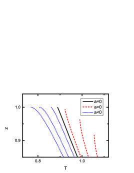
Figure 9: The relation between $z$ and $T$ for three-dimensional hard-sphere Bose gases in an isobaric process with different scattering length $a$. From left to right $a$ is gradually increased from negative to positive.

VII Conclusions

To sum up, in this paper, we present the explicit expression of the fugacity for two- and three-dimensional hard-sphere Bose and Fermi gases in isochoric and isobaric processes. The method is to convert the problem of solving the fugacity from the equation of state into the problem of finding the zero of a complex function based on the homogeneous Riemann-Hilbert problem. This method is introduced by Leonard for treating ideal quantum gases Leonard . Concretely, in this treatment, one can solve the fugacity $z$ from the relation

$$\Psi\left(\zeta\right)=\eta\left(\zeta-z\right){\displaystyle\prod\limits_{i=1}^{n_{\omega}-1}}\left(\zeta-\omega_{i}\right)\frac{\varphi\left(\zeta\right)}{{\displaystyle\prod\limits_{k=1}^{n}}\left(\zeta-c_{k}\right)^{\beta_{k}}},$$ (149)

where $z$ and $\omega_{i}$, $i=1,\cdots,n_{\omega}-1$, are the zeros of the complex function $\Psi\left(\zeta\right)$ which is constructed from the equation of state of quantum gases, $n_{\omega}$ is the number of the zeros, $c_{k}$ is the $k$-th end that is different from infinity of the boundary of the analytic region of $\Psi\left(\zeta\right)$, $n$ is the number of the ends different from infinity of the boundary, $\beta_{k}$ is a constant chosen to ensure that $\varphi\left(\zeta\right)$ is a fundamental solution and is determined by the behavior of $\Psi\left(\zeta\right)$ near the end $c_{k}$, and $\varphi\left(\zeta\right)$ is a fundamental solution of the homogeneous Riemann-Hilbert problem. By deriving both sides of this equation at a given point or setting various values of $\zeta$, one can obtain a set of equations of $z$, $\omega_{i}$, and the constant $\eta$. Solving such a set of equations gives the fugacity $z$.

The key steps in this treatment are (1) analytically continuing the real function $\Psi\left(z\right)$ whose zero corresponding to the fugacity $z$ to the whole complex plane, which gives the complex function $\Psi\left(\zeta\right)$, (2) finding the fundamental solution, and (3) determining the number of zeros of $\Psi\left(\zeta\right)$. At the first step, in the present case, the analytic continuation of $\Psi\left(z\right)$ relies on the analytic continuation of Bose-Einstein and Fermi-Dirac integrals; the analytically continued Bose-Einstein and Fermi-Dirac integrals are the polylogarithm (Jonquiére) functions, $Li_{\sigma}\left(\zeta\right)$ and $-Li_{\sigma}\left(-\zeta\right)$, respectively. At the second step, based on the result of the analytic continuation, we can analyze the singularity structure of $\Psi\left(\zeta\right)$, determine the boundary of the analytic region of $\Psi\left(\zeta\right)$, calculate the jump of $\Psi\left(\zeta\right)$ at the boundary, and then solve the fundamental solution $\varphi\left(\zeta\right)$. At the third step, though in general by the argument principle, one can only determine the difference between the number of zeros and the number of isolated singularities, one can determine the number of the zeros by use of the argument principle due to the fact that $\Psi\left(\zeta\right)$ has no isolated singularities in the present case.

It is worthy to point out that the explicit expression of the fugacity for the Bose case given in the present paper, especially the result for isobaric processes, can be directly applied to analyze the phase transition of the hard-sphere Bose gas system, which is an important problem in recent times hsb ; hsb2 . The reason is that the fugacity, and therefore the chemical potential, plays a central role in the theory of phase transitions, according to Erenfest’s theory of phase transitions. In the Erenfest classification, the order of a phase transition is defined by the order of the discontinuities in the derivatives of the Gibbs free energy, $G=N\mu$. Our results show that the transition temperature of the Bose-Einstein condensation can be obtained from the relations between the fugacity $z$ and the temperature $T$.

References

- (1) L. P. Kadanoff, Statistical Physics: Statics, Dynamics and Renormalization (World Scientific, Singapore, 2000).
- (2) K. Huang and C. N. Yang, Phys. Rev. 105, 767 (1957).
- (3) K. Huang, C. N. Yang, and J. M. Luttinger, Phys. Rev. 105, 776 (1957).
- (4) T. D. Lee and C. N. Yang, Phys. Rev. 116, 25 (1959). Before the publication of this paper, the results had been reported in T. D. Lee and C. N. Yang, Phys. Rev. 105, 1119 (1957).
- (5) W.-S. Dai and M. Xie, Europhys. Lett. 72, 887 (2005).
- (6) C. N. Yang, Europhys. Lett. 84, 40001 (2008).
- (7) B. B. Wei and C. N. Yang, Europhys. Lett. 87, 10005 (2009).
- (8) C. N. Yang, Chin. Phys. Lett. 26, 120504 (2009).
- (9) Z.-Q. Ma and C. N. Yang, Chin. Phys. Lett. 26, 120505 (2009).
- (10) Z.-Q. Ma and C. N. Yang, Chin. Phys. Lett. 26, 120506 (2009).
- (11) Z.-Q. Ma and C. N. Yang, Chin. Phys. Lett. 27, 020506 (2010).
- (12) Z.-Q. Ma and C. N. Yang, Chin. Phys. Lett. 27, 080501 (2010).
- (13) Z.-Q. Ma and C. N. Yang, Chin. Phys. Lett. 27, 090505 (2010).
- (14) C. N. Yang and Y. Z. You, Chin. Phys. Lett. 28, 020503 (2011).
- (15) M. Valiente, Europhys. Lett. 98, 10010 (2012).
- (16) A. Rançon and N. Dupuis, Phys. Rev. A 85, 063607 (2012).
- (17) H. Hu, X.-J. Liu, and P. D. Drummond, New J. Phys. 12, 063038 (2010).
- (18) F. A. de Saavedra, F. Mazzanti, J. Boronat, and A. Polls, Phys. Rev. A 85, 033615 (2012).
- (19) L. He and X.-G. Huang, Phys. Rev. A 85, 043624 (2012).
- (20) W.-S. Dai and M. Xie, Ann. Phys. (N. Y.) 322, 1771 (2007).
- (21) X.-J. Liu, H. Hu, and P.D. Drummond, Phys. Rev. B 82, 054524 (2010).
- (22) X.-J. Liu, H. Hu, and P.D. Drummond, Phys. Rev. Lett. 102, 160401 (2009).
- (23) B. Mihaila, J. F. Dawson, F. Cooper, C.-C. Chien, and E. Timmermans, Phys. Rev. A 83, 053637 (2011).
- (24) N. Sakumichi, N. Kawakami, and M. Ueda, Phys. Rev. A 85, 043601 (2012).
- (25) N. I. Muskhelishvili, Singular integral equations: Boundary problems of function theory and their application to mathematical physics, Revised translation from the Russian, edited by J. R. M. Radok (Noordhoff international publishing, Leyden, 1977).
- (26) A. Leonard, Phys. Rev. 175, 221 (1967).
- (27) W.-S. Dai and M. Xie, J. Stat. Mech. P07034 (2009).
- (28) W.-S. Dai and M. Xie, Ann. Phys. (N. Y.) 309, 295 (2004).
- (29) W.-S. Dai and M. Xie, J. Stat. Mech. P04021 (2009).
- (30) W.-S. Dai and M. Xie, Ann. Phys. (N. Y.) 332, 166 (2013).
- (31) W.-S. Dai and M. Xie, J. Math. Phys. 48 123302 (2007).
- (32) W.-S. Dai and M. Xie, Phys. Lett. A 311 340 (2003).
- (33) A. Sisman and I. Müller, Phys. Lett. A 320 360 (2004).
- (34) W.-S. Dai and M. Xie, Phys. Rev. E 70 016103, (2004).
- (35) A. Sisman, Z. F. Ozturk and C. Firat, Phys. Lett. A 362 16 (2007).
- (36) W.-S. Dai and M. Xie, JHEP 02 033 (2009).
- (37) C. Firat and A. Sisman, Phys. Scr. 87 045008 (2013).
- (38) A. Aydin, A. Sisman, Phys. Lett. A 378 2001 (2014).
- (39) A. Aydin, A. Sisman, Phys. Scr. 90 045208 (2015).
- (40) J. Clunie, Proc. Phys. Soc. A 67, 632 (1954).
- (41) W. Magnus, F. Oberhettinger, and R. P. Soni, Formulas and theorems for the special functions of mathematical physics, 3rd ed. (Springer-Verlag, Berlin, 1966).
- (42) D. C. Wood, Technical Report 15-92*, University of Kent, Computing Laboratory, University of Kent (Canterbury, UK, 1992).
- (43) J. O. Andersen, Rev. Mod. Phys. 76, 599 (2004).
- (44) R. Seiringer, Phys. Rev. B 80 014502 (2009).