Wake potentials and impedances of charged beams in gradually tapering structures

Abstract

We develop an analytical method for calculating the geometric wakefield and impedances of an ultrarelativistic beam propagating on- and off-axis through an axially symmetric geometry with slowly varying circular cross-section, such as a transition. Unlike previous analytical methods, our approach permits detailed perturbative investigation of geometric wakefields, and detailed perturbative investigation of impedance as a function of frequency. We compare the accuracy of the results of our approach with numerical simulations performed using the code ECHO and determine parameters in which there is good agreement with our asymptotic analysis.

I Introduction

Vital considerations in modern accelerator and light source design include the influence of non-uniform metallic structures, such as a vacuum system or collimator jaws, on nearby charged particle beams. Rapid changes in the spatial profile of the structure tend to have undesirable consequences for a particle beam, such as inducing instabilities and emittance growth; hence, designers often employ structures with cross-sections that gradually vary with distance. For example, a series of gradually tapering metallic structures (collimators) may be used to strip unwanted particles from beams prior to the collision event (see, for example, smith_glasman07 ).

Optimal design of particle accelerator subsystems is commonly sought by direct numerical solution of Maxwell’s equations, but accurate numerical computation of the electromagnetic fields near a short bunch in subsystems such as a post-linac collimator requires large computing resources beard_smith06 . In particular, numerically resolving a collimator with a gradually tapering geometry requires a mesh whose cells are much shorter than the length of the collimator. Although one may employ windowing techniques to avoid calculating the fields throughout the entire structure at every time step, such calculations frequently require intensive parallel computation  gjonaj06 ; smith09 . Similar problems are encountered when considering beam pipe transitions inside small-gap undulators in future light sources. In such cases, analytical expressions for the beam’s behaviour are highly desirable.

In practice, it is assumed that the beam does not deviate much from rectilinear motion parallel to the axis of the metallic structure chaobk . The beam’s trajectory is often obtained as a perturbation due to the coupling impedance of the unperturbed beam and structure (early discussions of impedances in tapered structures were given by Yokoya yokoya90 and Stupakov stupakov96 ). Although each frequency component of the unperturbed beam leads to its own impedance, it has been noted that low-frequency transverse impedance is dominated by the zero-frequency component of the source and longitudinal impedance is directly proportional to frequency over a broad frequency range stupakov96 . Recent work podobedov06 ; stupakov07 has been tailored to the above observations; it yields a frequency independent result for the transverse impedance and a longitudinal impedance directly proportional to frequency. Such methods do not permit detailed exploration of impedances as a function of frequency; the purpose of the following is to address this limitation.

To overcome the above, a new scheme for obtaining analytical expressions of impedances in gradually tapering, axially symmetric structures was suggested by us in burton08 . In common with podobedov06 ; stupakov07 , our approach employs an expansion in a small parameter $\epsilon$ characterising the gradually changing cross-sectional radius of the structure. However, we employ a decomposition of Maxwell’s equations using auxiliary potentials that yields impedance as a series in frequency, without a priori assuming that the frequency is small.

The following is an extensive investigation of the approach introduced in burton08 . We study the longitudinal and transverse wake potentials of a bunch travelling parallel to the axis of a perfectly conducting axially symmetric structure and compare the second, fourth and sixth order results in $\epsilon$ with numerical data from ECHO zagorodnov05 . We then present analytical expressions for longitudinal impedance; our method applied to a harmonic source reproduces the results given by Yokoya yokoya90 and Stupakov stupakov96 ; stupakov07 when working to second order in $\epsilon$. We also present corrections to the Yokoya-Stupakov results that arise due to higher order terms in $\epsilon$. Expressions for the longitudinal impedance up to fourth order in $\epsilon$ have been given previously in burton08 and we include them here for completeness. We then turn to a detailed exposition of the passage from Maxwell’s equations to our iterative procedure for calculating auxiliary potentials order-by-order in $\epsilon$. A discussion of the difficulties encountered when auxiliary potentials are not used is given in Appendix B.

II Overview and results

A full account of our solution method is presented in later sections. This section focusses on a comparison of the results obtained using our asymptotic method and results obtained using the code ECHO.

Our investigation concentrates on beams propagating through axially symmetric structures whose circular cross-sections gradually change along the axis of symmetry. Such structures are topologically equivalent to an infinite right circular cylinder and we call them waveguides (see Figure 1). This article focusses entirely on the geometric wake of the beam in the inductive regime tenenbaum:2007 . Here, the walls of the waveguide are assumed to be perfectly conducting; resistive effects will be considered elsewhere.

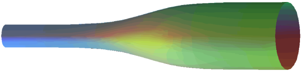
Figure 1: A waveguide with a slowly varying profile

We develop the electromagnetic field of the beam as an asymptotic expansion in a small parameter $\epsilon$ characterising the gradually changing radius of a waveguide with a smoothly varying profile. In particular, the radial profile of the waveguide is specified as

$$r=R(z)=\check{R}(\epsilon z)$$ (1)

where $\epsilon\ll 1$ and $(r,\theta,z)$ is a cylindrical coordinate system with $z$ a Cartesian coordinate parallel to the waveguide’s axis of symmetry ($r=0$).

The two radial profiles explored here numerically are

$$r=R(z)=20-18\exp[-z^{2}/(8\times 10^{5}l^{2})]$$ (2)

with $\epsilon=1/\sqrt{8\times 10^{5}}$ and

$$r=R(z)=20-18\textrm{ sech }(0.01z/l)$$ (3)

where $\epsilon=0.01$. The coordinates $z,r$ and the constant $l$ have dimensions of length; in the following $l=1\text{mm}$, and $z,r$ are measured in mm. The profiles (2, 3) have a ratio of gap to beam pipe radius and average taper gradient similar to that proposed for the beam delivery system of the next generation of lepton colliders tenenbaum:2007 .

Wake potentials are calculated by integrating components of the electromagnetic field along a straight line parallel to the axis of the waveguide. We consider fields excited by a narrow Gaussian bunch of effective length $\sigma$ propagating at the speed of light parallel to the waveguide’s axis, offset by a distance $r_{0}$ from the waveguide’s axis. The charge density $\rho$ of the bunch is

$$\rho_{r_{0},\theta_{0}}(r,\theta,u)=\frac{q_{0}e^{-\frac{u^{2}}{2\sigma^{2}}}}{\sigma\sqrt{2\pi}}\delta\left(x-r_{0}\cos\theta_{0}\right)\delta\left(y-r_{0}\sin\theta_{0}\right)$$ (4)

where $u=z-ct$, $x=r\cos\theta$, $y=r\sin\theta$ and $q_{0}$ is the total charge of the bunch. The longitudinal wake potential $W^{\parallel}$ is given by

$$W^{\parallel}(r,\theta,u)=-\frac{1}{q_{0}}\int_{-\infty}^{\infty}E_{z}\big{|}_{ct=z-u}\,dz$$ (5)

where

$$E_{z}\big{|}_{ct=z-u}=E_{z}\left(r,\theta,z,t=\frac{z-u}{c}\right)$$ (6)

and $E_{z}$ is the longitudinal (i.e. $z$) component of the electric field. The transverse wake potential ${\bf W}_{\perp}$ may be obtained from $W^{\parallel}$ using the Panofsky-Wenzel relation panofsky56 .

Sample results for $W^{\parallel}$ are shown in Figures 2, 3. The “leading order” curves result from electromagnetic fields calculated up to 2nd order in $\epsilon$, while the “4th order” and “6th order” curves arise from including 4th order and 6th order corrections in $\epsilon$ respectively. It may be shown that the 3rd, 5th and 7th order contributions to $W^{\parallel}$ vanish.

Wake potentials can be calculated from impedances using Fourier methods zotter_kheifets98 and the leading order results may be recovered using well-known expressions for impedance originally due to Yokoya yokoya90 . Corrections to the leading order transverse impedance that properly accommodate the waveguide’s taper but neglect the frequency dependence of the source may be found in podobedov06 ; we expect the frequency dependences of impedances to be more accurately represented using our method.

Data from ECHO was obtained for a sequence of mesh cell densities ($10,15,20$ cells over bunch length $\sigma$; we judged the numerical errors to be small based on the small differences between the results for $10$, $15$ and $20$ cells per $\sigma$). The monopole and dipole contributions to (4) are the zeroth and first order terms in an expansion of (4) with respect to $r_{0}$; for direct comparison with the ECHO data, only the wake potentials due the monopole and dipole contributions are calculated.

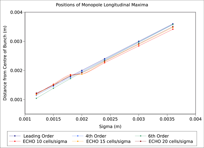
Figure 5: The position of the maximum in $u$ of $W^{\parallel}$ versus effective bunch length $\sigma$ for a monopole source propagating through the exponential geometry (2).

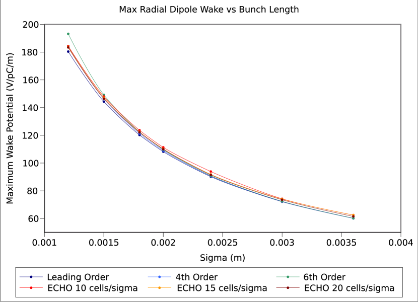
Figure 6: The maximum in $u$ of the radial component of ${\bf W}_{\perp}$ versus effective bunch length $\sigma$ for a dipole source propagating through the exponential geometry (2).

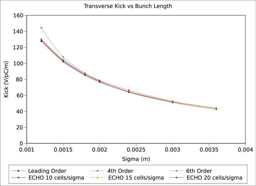
Figure 7: The transverse momentum kick versus effective bunch length $\sigma$ for a dipole source propagating through the exponential geometry (2).

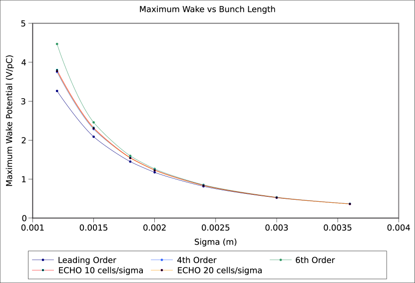
Figure 8: The maximum in $u$ of $W^{\parallel}$ versus effective bunch length $\sigma$ for a monopole source propagating through the hyperbolic secant geometry (3).

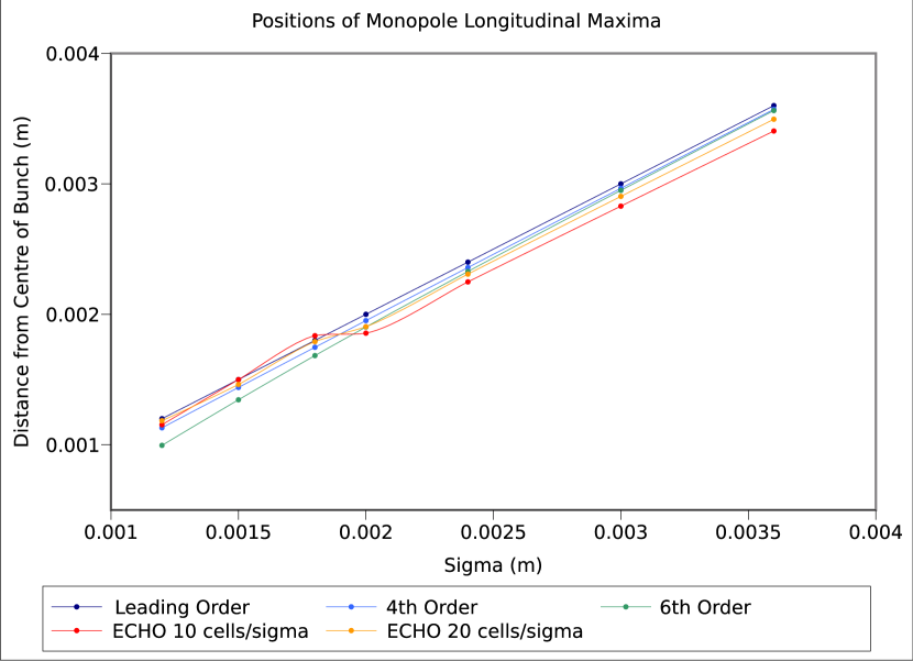
Figure 9: The position of the maximum in $u$ of $W^{\parallel}$ versus effective bunch length $\sigma$ for a monopole source propagating through the hyperbolic secant geometry (3).

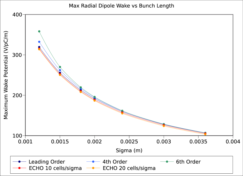
Figure 10: The maximum in $u$ of the radial component of ${\bf W}_{\perp}$ versus effective bunch length $\sigma$ for a dipole source propagating through the hyperbolic secant geometry (3).

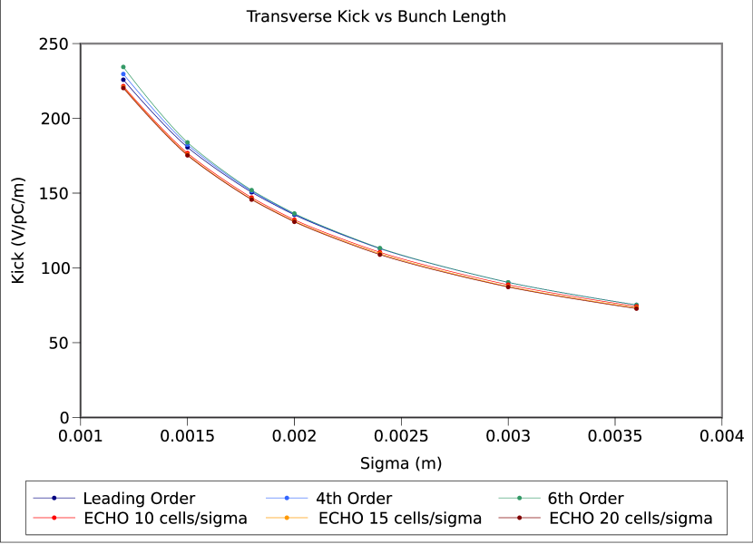
Figure 11: The transverse momentum kick versus effective bunch length $\sigma$ for a dipole source propagating through the hyperbolic secant geometry (3).

Figures (4-7) show the magnitude and position of the maxima of longitudinal wake potentials, the magnitude of the maxima of the radial component of transverse wake potentials and the momentum kicks induced by transverse wakes in the exponential geometry. Figures (8-11) show the corresponding quantities for the sech profile. The higher order contributions reduce in significance as the effective bunch length $\sigma$ increases and we observe that the 4th and 6th order results agree well with the leading order predictions for bunch lengths longer than $\sim 2\text{mm}$. For $\sigma$ less than $\sim 1.5\text{mm}$ the data shows that, in a number of cases, the maximum values of the wake potentials and momentum kicks obtained using ECHO generally agree better with the 4th order results than with the leading order (Yokoya-Stupakov) predictions over the parameter ranges considered here. The sample plots of $W^{\parallel}$ shown in Figures 2, 3 demonstrate this for a bunch length of $1.2\text{mm}$; for such bunch lengths the reliability of the 6th order correction is questionable. Although the agreement with the numerical results is impressive, we warn the reader that the radius of convergence of our perturbative expansion is unknown.

II.1 Impedance of an on-axis beam

In this section we present impedance formulae due to the on-axis harmonic charge density

$$\varrho_{\omega}(r,\theta,u)=\frac{I_{\omega}}{c}e^{\frac{i\omega u}{c}}\delta(x)\delta(y)$$ (7)

where $I_{\omega}$ defines the harmonic current component of the beam. The longitudinal impedance $Z^{\parallel}(\omega)$ for angular frequency $\omega$ is

$$Z^{\parallel}(\omega)=-\frac{1}{I_{\omega}}\int_{-\infty}^{\infty}{e^{-\frac{i\omega u}{c}}E_{z}\big{|}_{ct=z-u}\ \mathrm{d}z}$$ (8)

where $E_{z}$ is the longitudinal component of the electric field generated by the source (7). The approach detailed in subsequent sections leads to the following :

$$Z^{\parallel}_{\text{on-axis}}(\omega)=Z^{\parallel}_{1\,\text{on-axis}}+Z^{\parallel}_{2\,\text{on-axis}}+Z^{\parallel}_{4\,\text{on-axis}}+Z^{\parallel}_{6\,\text{on-axis}}+\dots$$ (9)

where $Z^{\parallel}_{1\,\text{on-axis}}+Z^{\parallel}_{2\,\text{on-axis}}$ is the Yokoya-Stupakov longitudinal geometric impedance

$$Z^{\parallel}_{1\,\text{on-axis}}=\frac{1}{2\pi\varepsilon_{0}c}\ln\left(\frac{R_{1}}{R_{2}}\right),$$ (10)

$$Z^{\parallel}_{2\,\text{on-axis}}=-\frac{i\omega}{4\pi\varepsilon_{0}c^{2}}\int_{-\infty}^{\infty}{R^{\prime 2}\mathrm{d}z}$$ (11)

with $R^{\prime}=dR/dz$, $R_{1}=R(\infty)$ and $R_{2}=R(-\infty)$. Equations (10, 11) follow, respectively, from 1st and 2nd order terms in $\epsilon$ in an asymptotic series for $E_{z}$. The corrections

$$4\pi\varepsilon_{0}cZ^{\parallel}_{4\,\text{on-axis}}=\frac{i\omega}{24c}\int_{-\infty}^{\infty}\bigg{\{}5R^{\prime 4}+3\left(R\,R^{\prime\prime}\right)^{2}-2\frac{\omega^{2}}{c^{2}}\left(R^{2}\,R^{\prime\prime}\right)^{2}\bigg{\}}\mathrm{d}z$$ (12)

and

$$4\pi\varepsilon_{0}cZ^{\parallel}_{6\,\text{on-axis}}= -\frac{i\omega}{c}\int_{-\infty}^{\infty}\bigg{\{}\frac{3}{16}(R^{\prime\prime}\,R^{\prime}\,R)^{2}+\frac{11}{120}R^{\prime 6}+\frac{1}{48}(R^{2}\,R^{\prime\prime\prime})^{2}\bigg{\}}\mathrm{d}z$$

$$+\frac{i\omega^{3}}{c^{3}}\int_{-\infty}^{\infty}\bigg{\{}\frac{11}{256}\left(R^{3}\,R^{\prime\prime\prime}\right)^{2}-\frac{1}{6}\left(R^{2}\,R^{\prime}\,R^{\prime\prime}\right)^{2}-\frac{73}{768}R^{5}\,R^{\prime\prime 3}\bigg{\}}\mathrm{d}z$$

$$+\frac{i\omega^{5}}{c^{5}}\int_{-\infty}^{\infty}\bigg{\{}\frac{19}{160}(R^{3}\,R^{\prime}\,R^{\prime\prime})^{2}+\frac{73}{1920}R^{7}\,R^{\prime\prime 3}-\frac{19}{1920}(R^{\prime\prime\prime}\,R^{4})^{2}\bigg{\}}\mathrm{d}z$$ (13)

arise from 4th and 6th order terms in the asymptotic series for $E_{z}$. The imaginary part of $Z^{\parallel}$ is invariant under reversal of the direction of the beam, i.e. $\text{Im}(Z^{\parallel})$ is invariant under the replacement $R(z)\mapsto R(-z)$. Thus, each term in the integrand in $\text{Im}(Z^{\parallel})$ only contains an even number of derivatives of $R$ and arises from an even power of $\epsilon$ in the asymptotic series for $E_{z}$. It follows that the odd order contributions to $\text{Im}(Z^{\parallel})$ vanish.

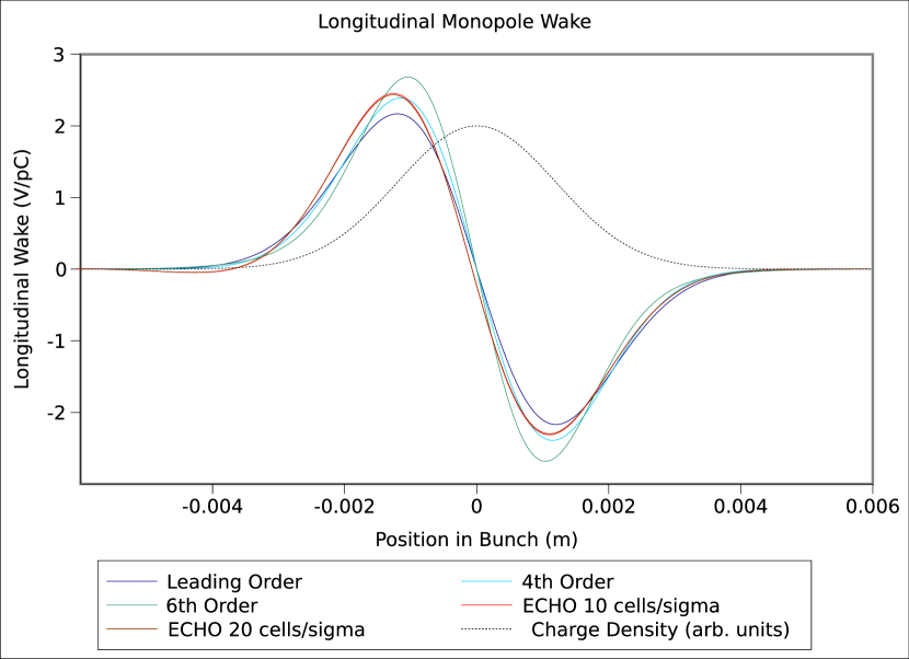
Figure 2: Sample longitudinal wake potential $W^{\parallel}$ versus $u=z-ct$ for an on-axis source (length $1.2\text{mm}$) propagating through the exponential geometry (2).

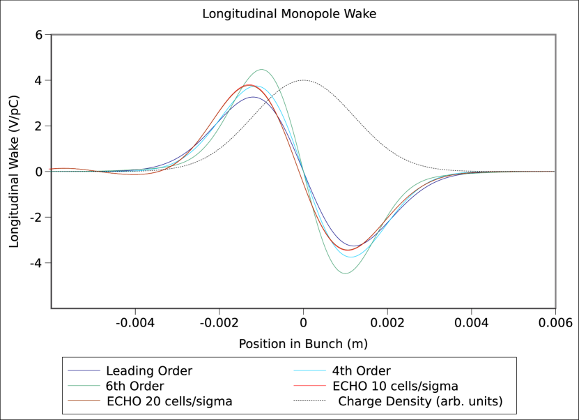
Figure 3: Sample longitudinal wake potential $W^{\parallel}$ versus $u=z-ct$ for an on-axis source (length $1.2\text{mm}$) propagating through the hyperbolic secant geometry (3).

II.2 Impedance of an off-axis beam

This section focusses on longitudinal impedance due to the off-axis harmonic line charge density

$$\varrho_{\omega,r_{0},\theta_{0}}(r,\theta,u)=\frac{I_{\omega}}{c}e^{i\omega u}\delta\left(x-r_{0}\cos\theta_{0}\right)\delta\left(y-r_{0}\sin\theta_{0}\right)$$ (14)

where $r_{0}\neq 0$. The corresponding transverse impedance ${\bf Z}_{\perp}$ may be obtained using the Panofsky-Wenzel relation panofsky56 .

Fourier expansion of the source in $\theta$ leads to

$$Z^{\parallel}(\omega)=Z^{\parallel}_{\text{on-axis}}+Z^{\parallel}_{1}+Z^{\parallel}_{2}+Z^{\parallel}_{4}+Z^{\parallel}_{6}+\dots$$ (15)

where $Z^{\parallel}_{\text{on-axis}}$ (see (9)) is the monopole contribution to $Z^{\parallel}$ and the contributions arising from 1st, 2nd, 4th and 6th-order terms in $E_{z}$ are

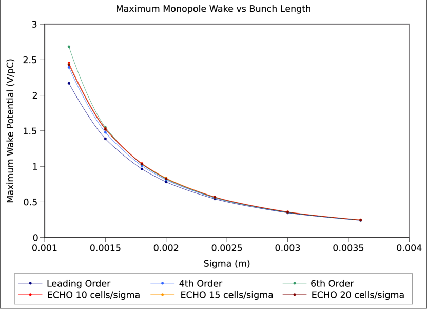
Figure 4: The maximum in $u$ of $W^{\parallel}$ versus effective bunch length $\sigma$ for a monopole source propagating through the exponential geometry (2).

$$Z^{\parallel}_{1}=\frac{1}{4\pi\varepsilon_{0}c}\sum_{m=1}^{\infty}\frac{2}{m}\bigg{(}\frac{1}{R_{2}^{2m}}-\frac{1}{R_{1}^{2m}}\bigg{)}\,r^{m}r_{0}^{m}\cos m(\theta-\theta_{0}),$$ (16)

$$Z^{\parallel}_{2}=\frac{1}{4\pi\varepsilon_{0}c^{2}}\sum_{m=1}^{\infty}\Bigg{\{}-\frac{4i\omega}{1+m}\int_{-\infty}^{\infty}{\left(\frac{R^{\prime}}{R^{m}}\right)^{2}\mathrm{d}z\Bigg{\}}}r^{m}r_{0}^{m}\cos m(\theta-\theta_{0}),$$ (17)

$$4\pi\varepsilon_{0}cZ^{\parallel}_{4}=\sum_{m=1}^{\infty}\frac{2i\omega}{c}\frac{r_{0}^{m}r^{m}\cos m(\theta-\theta_{0})}{m(m+1)(m+2)}\Bigg{\{}\int_{-\infty}^{\infty}{\left(\frac{R^{\prime 4}}{R^{2m}}\frac{2m^{2}+6m+1}{3}+\frac{R^{\prime\prime 2}}{R^{2m-2}}\right)\mathrm{d}z}$$

$$\qquad-\frac{\omega^{2}}{c^{2}}\frac{3m^{2}+8m+6}{m(m+1)^{2}(m+3)}\int_{-\infty}^{\infty}{\left(\frac{4m-3}{3}\frac{R^{\prime 4}}{R^{2m-2}}+\frac{R^{\prime\prime 2}}{R^{2m-4}}\right)\mathrm{d}z}\Bigg{\}},$$ (18)

$$4\pi\varepsilon_{0}cZ^{\parallel}_{6}= \sum_{m=1}^{\infty}\frac{i\omega}{c}\frac{r_{0}^{m}r^{m}\cos m(\theta-\theta_{0})}{10m^{2}(m+1)^{3}(m+2)(m+3)}\int_{-\infty}^{\infty}\Bigg{\{}5(m^{2}+8m+6)\frac{R^{\prime\prime\prime 2}}{R^{2m-4}}$$

$$+5(10m^{3}+14m^{2}-9m-18)\frac{R^{\prime\prime 3}}{R^{2m-3}}+15m(2m^{3}+20m^{2}+41m+27)\frac{R^{\prime\prime 2}R^{\prime 2}}{R^{2m-2}}$$

$$+2m(4m^{5}+32m^{4}+99m^{3}+137m^{2}+85m+15)\frac{R^{\prime 6}}{R^{2m}}+\frac{\omega^{2}}{c^{2}m(m+4)}\Bigg{[}30(5m^{2}+20m+24)\frac{R^{\prime\prime\prime 2}}{R^{2m-6}}$$

$$+20(23m^{3}+40m^{2}-58m-156)\frac{R^{\prime\prime 3}}{R^{2m-5}}+10(236m^{3}+693m^{2}+304m-816)\frac{R^{\prime 2}R^{\prime\prime 2}}{R^{2m-4}}$$

$$+4(154m^{4}+375m^{3}-2m^{2}-628m+240)\frac{R^{\prime 6}}{R^{2m-2}}+\frac{\omega^{2}}{c^{2}m(m+1)^{2}(m+2)(m+5)}\times$$

$$\Bigg{[}-5(35m^{5}+351m^{4}+1428m^{3}+2836m^{2}+2672m+960)\frac{R^{\prime\prime\prime 2}}{R^{2m-8}}$$

$$-5(106m^{6}+756m^{5}+1639m^{4}-923m^{3}-8636m^{2}-11440m-4800)\frac{R^{\prime\prime 3}}{R^{2m-7}}$$

$$+5(30m^{7}-378m^{6}-4395m^{5}-14574m^{4}-13667m^{3}+19680m^{2}+43424m+21120)\frac{R^{\prime 2}R^{\prime\prime 2}}{R^{2m-6}}$$

$$+(m-1)(60m^{7}-33m^{6}-2713m^{5}-10453m^{4}-9129m^{3}$$

$$+19912m^{2}+40000m+19200)\frac{R^{\prime 6}}{R^{2m-4}}\Bigg{]}\Bigg{]}\Bigg{\}}\mathrm{d}z$$ (19)

respectively, where $m$ is the multipole index. Since $\text{Im}(Z^{\parallel})$ is invariant under the replacement $R(z)\mapsto R(-z)$, i.e. invariant under reversal of the direction of the beam, the odd order terms in the asymptotic expansion of $\text{Im}(Z^{\parallel})$ in $\epsilon$ vanish.

The longitudinal impedance of a dipole source is obtained by setting $m=1$ in (16, 17, 18, 19):

$$4\pi\epsilon_{0}cZ_{1}^{\parallel}=2\left(\frac{1}{R_{2}}-\frac{1}{R_{1}}\right)r_{0}r\cos(\theta-\theta_{0}),$$ (20)

$$4\pi\epsilon_{0}cZ_{2}^{\parallel}=-2i\frac{\omega}{c}r_{0}r\cos(\theta-\theta_{0})\int_{-\infty}^{\infty}\frac{R^{\prime 2}}{R^{2}}\mathrm{d}z,$$ (21)

$$4\pi\epsilon_{0}cZ_{4}^{\parallel}=i\frac{\omega}{c}r_{0}r\cos(\theta-\theta_{0})\Bigg{[}\int_{-\infty}^{\infty}{\left(\frac{{R^{\prime}}^{4}}{R^{2}}+\frac{1}{3}{R^{\prime\prime}}^{2}\right)\mathrm{d}z}-\frac{\omega^{2}}{c^{2}}\int_{-\infty}^{\infty}{\left(\frac{17}{144}{R^{\prime}}^{4}+\frac{17}{48}{R^{\prime\prime}}^{2}R^{2}\right)\mathrm{d}z}\Bigg{]},$$ (22)

$$4\pi\epsilon_{0}cZ_{6}^{\parallel}=i\frac{\omega}{c}r_{0}r\cos(\theta-\theta_{0})\Bigg{[}\int_{-\infty}^{\infty}{\left(-\frac{31}{40}\frac{{R^{\prime}}^{6}}{R^{2}}-\frac{45}{32}{R^{\prime}}^{2}{R^{\prime\prime}}^{2}-\frac{17}{192}{R^{\prime\prime\prime}}^{2}R^{2}+\frac{1}{64}{R^{\prime\prime}}^{3}R\right)\mathrm{d}z}$$

$$\qquad\qquad+\frac{\omega^{2}}{c^{2}}\int_{-\infty}^{\infty}{\left(\frac{139}{1200}{R^{\prime}}^{6}+\frac{139}{160}{R^{\prime\prime}}^{2}{R^{\prime}}^{2}R^{2}+\frac{49}{160}{R^{\prime\prime\prime}}^{2}R^{4}-\frac{151}{240}{R^{\prime\prime}}^{3}R^{3}\right)\mathrm{d}z}$$

$$\qquad\qquad+\frac{\omega^{4}}{c^{4}}\int_{-\infty}^{\infty}{\left(-\frac{4141}{34560}{R^{\prime\prime\prime}}^{2}R^{6}+\frac{3883}{11520}{R^{\prime\prime}}^{3}R^{5}+\frac{427}{576}{R^{\prime\prime}}^{2}{R^{\prime}}^{2}R^{4}\right)\mathrm{d}z}\Bigg{]}.$$ (23)

Use of the Panofsky-Wenzel relation panofsky56 and (20, 21, 22, 23) leads to the following contributions to the transverse dipole impedance $Z^{\perp}(\omega)$:

$$4\pi\epsilon_{0}cZ_{1}^{\perp}=\frac{2c}{\omega}\left(\frac{1}{R_{2}}-\frac{1}{R_{1}}\right),$$ (24)

$$4\pi\epsilon_{0}cZ_{2}^{\perp}=-2i\int_{-\infty}^{\infty}\frac{R^{\prime 2}}{R^{2}}\mathrm{d}z,$$ (25)

$$4\pi\epsilon_{0}cZ_{4}^{\perp}=i\Bigg{[}\int_{-\infty}^{\infty}{\left(\frac{{R^{\prime}}^{4}}{R^{2}}+\frac{1}{3}{R^{\prime\prime}}^{2}\right)\mathrm{d}z}-\frac{\omega^{2}}{c^{2}}\int_{-\infty}^{\infty}{\left(\frac{17}{144}{R^{\prime}}^{4}+\frac{17}{48}{R^{\prime\prime}}^{2}R^{2}\right)\mathrm{d}z}\Bigg{]},$$ (26)

$$4\pi\epsilon_{0}cZ_{6}^{\perp}= i\Bigg{[}\int_{-\infty}^{\infty}{\left(-\frac{31}{40}\frac{{R^{\prime}}^{6}}{R^{2}}-\frac{45}{32}{R^{\prime}}^{2}{R^{\prime\prime}}^{2}-\frac{17}{192}{R^{\prime\prime\prime}}^{2}R^{2}+\frac{1}{64}{R^{\prime\prime}}^{3}R\right)\mathrm{d}z}$$

$$+\frac{\omega^{2}}{c^{2}}\int_{-\infty}^{\infty}{\left(\frac{139}{1200}{R^{\prime}}^{6}+\frac{139}{160}{R^{\prime\prime}}^{2}{R^{\prime}}^{2}R^{2}+\frac{49}{160}{R^{\prime\prime\prime}}^{2}R^{4}-\frac{151}{240}{R^{\prime\prime}}^{3}R^{3}\right)\mathrm{d}z}$$

$$+\frac{\omega^{4}}{c^{4}}\int_{-\infty}^{\infty}{\left(-\frac{4141}{34560}{R^{\prime\prime\prime}}^{2}R^{6}+\frac{3883}{11520}{R^{\prime\prime}}^{3}R^{5}+\frac{427}{576}{R^{\prime\prime}}^{2}{R^{\prime}}^{2}R^{4}\right)\mathrm{d}z}\Bigg{]}$$ (27)

where

$$Z^{\perp}(\omega)=Z^{\perp}_{1}+Z^{\perp}_{2}+Z^{\perp}_{4}+Z^{\perp}_{6}+\dots.$$ (28)

The imaginary part of the transverse impedance at zero frequency $\lim_{\omega\rightarrow 0}\text{Im}[Z^{\perp}(\omega)]$ was previously obtained in podobedov06 . As far as we are aware, the above expressions for transverse impedance as a function of frequency are new.

III Derivation of results

The remainder of the paper focusses on the method used to derive the expressions presented above.

III.1 Decomposition of Maxwell’s equations using auxiliary potentials

III.1.1 2+2 split of Maxwell’s equations

The approach we use is based on a 2+2 split of Maxwell’s equations adapted to the waveguide. We employ cylindrical polar co-ordinates $(t,r,\theta,z)$ on Minkowski spacetime where $r=0$ is the waveguide’s axis, $\theta$ is the azimuthal angle around the waveguide’s axis and $z$ is a co-ordinate parallel to the waveguide’s axis. We employ exterior differential calculus to analyse Maxwell’s equations (see, for example, benn_tucker87 ; burton03 ) as it affords a concise language for exploiting different coordinate systems and for developing our new auxiliary potential method discussed in the following.

Let $({\cal M},g)$ be Minkowski spacetime where $g$ is the metric

$$g=-c^{2}\mathrm{d}t\otimes\mathrm{d}t+\mathrm{d}z\otimes\mathrm{d}z+\mathrm{d}r\otimes\mathrm{d}r+r^{2}\mathrm{d}\theta\otimes\mathrm{d}\theta$$ (29)

in $(t,r,\theta,z)$ co-ordinates. We choose the volume $4$-form $\star 1$ as

$$\star 1=c\mathrm{d}t\wedge\mathrm{d}z\wedge\#_{\perp}1$$ (30)

where the $2$-form $\#_{\perp}1$,

$$\#_{\perp}1=r^{2}\mathrm{d}r\wedge\mathrm{d}\theta,$$ (31)

and the metric $g_{\perp}$,

$$g_{\perp}=\mathrm{d}r\otimes\mathrm{d}r+r^{2}\mathrm{d}\theta\otimes\mathrm{d}\theta,$$ (32)

are adapted to constant $(t,z)$ surfaces inside the waveguide. The waveguide surface in ${\cal M}$ is the $3$-dimensional hypersurface $\{r=R(z)\,|\,-\infty<z<\infty\}$ where $R(z)$ is the radius of the cross-section at $z$ with unit normal $\partial_{z}$.

The source moves in the positive $z$-direction near the speed of light in the laboratory frame, and its $4$-velocity field $V$ is well-approximated by the null vector :

$$V=\frac{1}{c}\partial_{t}+\partial_{z}.$$ (33)

The metric isomorphism between the spaces of vectors and co-vectors on spacetime is denoted as follows: the co-vector field $\widetilde{X}$ associated with the vector field $X$ is defined such that $\widetilde{X}(Y)=g(X,Y)$ for all vector fields $Y$ and the vector field $\widetilde{\alpha}$ associated with the co-vector field $\alpha$ is defined such that $\beta(\widetilde{\alpha})=g^{-1}(\beta,\alpha)$ for all co-vector fields $\beta$. Hence, the $1$-form $\widetilde{V}$ associated with $V$ is

$$\widetilde{V}=\mathrm{d}z-c\mathrm{d}t.$$ (34)

It is expedient to transform to a new co-ordinate chart:

$$u=z-ct,\qquad\zeta=z$$ (35)

with

$$g=\mathrm{d}\zeta\otimes\mathrm{d}u+\mathrm{d}u\otimes\mathrm{d}\zeta-\mathrm{d}u\otimes\mathrm{d}u+g_{\perp},$$ (36)

$$\star 1=\mathrm{d}\zeta\wedge\mathrm{d}u\wedge\#_{\perp}1.$$ (37)

The coordinates (35) play a useful role because the source is naturally expressed in terms of $u$ and the boundary of the waveguide is described using $\zeta$. It follows that

$$\widetilde{V}=\mathrm{d}u,$$ (38)

$$\star\widetilde{V}=\mathrm{d}u\wedge\#_{\perp}1.$$ (39)

Here, the Hodge map $\star$ on $\cal{M}$ satisfies

$$\star(\nu\wedge\widetilde{X})=\mathrm{i}_{X}\star\nu$$ (40)

where $\nu$ is an arbitrary form and $X$ is an arbitrary vector field and $\mathrm{i}_{X}$ is the interior contraction with $X$. The transverse Hodge map $\#_{\perp}$ is defined on the transverse, cross-sectional subspace to satisfy

$$\#_{\perp}(\mu_{\perp}\wedge\widetilde{Y})=\mathrm{i}_{Y}\#_{\perp}\mu_{\perp}$$ (41)

where $\mu_{\perp}$ is a form on the domain spanned by $\{\mathrm{d}r,\mathrm{d}\theta\}$ and $Y$ is a vector field in the span of $\{\partial_{r},\partial_{\theta}\}$.

The Maxwell equations on space-time are

$$\mathrm{d}F=0$$ (42)

$$\varepsilon_{0}\mathrm{d}\star F=-\varrho\star\widetilde{V}$$ (43)

where $\varrho\widetilde{V}$ is the electric $4$-current of the beam and $\mathrm{d}$ is the exterior derivative on forms. Charge conservation

$$\mathrm{d}(\varrho\star\widetilde{V})=0$$ (44)

yields

$$\partial_{\zeta}\varrho=0.$$ (45)

Without loss of generality, the electromagnetic $2$-form $F$ is decomposed as

$$F=\Phi\mathrm{d}\zeta\wedge\mathrm{d}u+\mathrm{d}u\wedge\alpha+\mathrm{d}\zeta\wedge\beta+\Psi\#_{\perp}1$$ (46)

where $\alpha$ and $\beta$ lie in the subspace of $1$-forms spanned by $\{\mathrm{d}r,\,\mathrm{d}\theta\}$ (transverse subspace). The component $\Phi$ of $F$ is the longitudinal component of the electric field in $\left(r,\theta,u,\zeta\right)$ coordinates:

$$E_{z}\left(r,\theta,z=\zeta,t=\frac{1}{c}(\zeta-u)\right)=\Phi(r,\theta,u,\zeta).$$ (47)

(See, for example, burton07 for a detailed discussion of the relationship between $F$ and electric and magnetic fields in vector notation). It follows that the Maxwell equations (42) and (43) can be decomposed as

$$\mathrm{d}_{\perp}\Phi+\partial_{\zeta}\alpha-\partial_{u}\beta=0,$$ (48)

$$\partial_{\zeta}\Psi\#_{\perp}1-\mathrm{d}_{\perp}\beta=0,$$ (49)

$$\partial_{u}\Psi\#_{\perp}1-\mathrm{d}_{\perp}\alpha=0,$$ (50)

$$\partial_{\zeta}\#_{\perp}(\alpha+\beta)+\partial_{u}\#_{\perp}\beta-\mathrm{d}_{\perp}\Psi=0,$$ (51)

$$\mathrm{d}_{\perp}\#_{\perp}(\alpha+\beta)-\partial_{u}\Phi\#_{\perp}1=-\rho(r,\theta,u)\#_{\perp}1,$$ (52)

$$\partial_{\zeta}\Phi\#_{\perp}1+\mathrm{d}_{\perp}\#_{\perp}\beta=0$$ (53)

where $\mathrm{d}_{\perp}$ is the exterior derivative acting in the transverse subspace, and $\rho(r,\theta,u)\equiv\frac{1}{\varepsilon_{0}}\varrho(r,\theta,u)$, the functional dependence of the charge density being written explicitly to emphasize its independence of $\zeta$ due to (45).

III.1.2 Auxiliary potentials

In this section we introduce a set of six 0-forms (auxiliary potentials). This anticipates the imposition of the perturbation scheme in Section III.4: they will be shown to satisfy tractable second order PDEs in gradually tapering waveguides, whereas working directly with the conventional electromagnetic potentials leads to third order PDEs. Appendix B contains a brief discussion of this issue.

After rewriting the Maxwell equations in terms of auxiliary potentials, and adopting perfectly conducting boundary conditions, we will show that asymptotic expansions of the auxiliary potentials yield 2-dimensional Poisson and Laplace equations at each order in the expansion parameter $\epsilon$.

In Appendix A, we demonstrate that the transverse 1-forms $\alpha$ and $\beta$ can be replaced by the $0$-form pairs $\{A,a\}$ and $\{B,b\}$, viz.

$$\alpha=\mathrm{d}_{\perp}A+\#_{\perp}\mathrm{d}_{\perp}a,$$ (54)

$$\beta=\mathrm{d}_{\perp}B+\#_{\perp}\mathrm{d}_{\perp}b$$ (55)

where $A$ and $B$ obey Dirichlet boundary conditions on the waveguide boundary, i.e. $A=B=0$ at $r=R(\zeta)$.

It follows that (since $\mathrm{d}^{2}=0$) the Maxwell equations (48-53) partially decouple to give

$$\mathrm{d}_{\perp}\left(\Phi+\partial_{\zeta}A-\partial_{u}B\right)+\#_{\perp}\mathrm{d}_{\perp}\left(\partial_{\zeta}a-\partial_{u}b\right)=0,$$ (56)

$$\partial_{\zeta}\Psi+\delta_{\perp}\mathrm{d}_{\perp}b=0,$$ (57)

$$\partial_{u}\Psi+\delta_{\perp}\mathrm{d}_{\perp}a=0,$$ (58)

$$\mathrm{d}_{\perp}\left(\partial_{\zeta}(A+B)+\partial_{u}B\right)+\#_{\perp}\mathrm{d}_{\perp}\left(\Psi+\partial_{\zeta}(a+b)+\partial_{u}b\right)=0,$$ (59)

$$\delta_{\perp}\mathrm{d}_{\perp}(A+B)+\partial_{u}\Phi=\rho(r,\theta,u),$$ (60)

$$\partial_{\zeta}\Phi-\delta_{\perp}\mathrm{d}_{\perp}B=0,$$ (61)

where

$$\delta_{\perp}\mu_{\perp}\equiv(-1)^{p}\#_{\perp}^{-1}\mathrm{d}_{\perp}\#_{\perp}\mu_{\perp}$$ (62)

is the transverse co-derivative of a transverse (i.e. in the span of $\{\mathrm{d}r,\mathrm{d}\theta\}$) $p$-form $\mu_{\perp}$ and $\#_{\perp}^{-1}\#_{\perp}=\#_{\perp}\#_{\perp}^{-1}=1$.

Motivated by the appearance of equations (56) and (59), introduce $0$-forms $\{\mathcal{H}^{\Phi}$, $\mathcal{H}^{\varphi}$, $\mathcal{H}^{B}$, $\mathcal{H}^{b}$, $\hat{W}$, $\hat{X}\}$ that satisfy

$$\partial_{u}\mathcal{H}^{\Phi}=\Phi+\partial_{\zeta}A-\partial_{u}B,$$ (63)

$$\partial_{u}\mathcal{H}^{\varphi}=\partial_{\zeta}a-\partial_{u}b,$$ (64)

$$\partial_{u}\mathcal{H}^{B}=\partial_{\zeta}(A+B)+\partial_{u}B,$$ (65)

$$\mathcal{H}^{b}=\Psi+\partial_{\zeta}(a+b)+\partial_{u}b,$$ (66)

$$\partial_{u}\hat{W}=A+B,$$ (67)

$$\partial_{u}\hat{X}=a.$$ (68)

Equations (63-68) do not specify $\{\mathcal{H}^{\Phi},\mathcal{H}^{\varphi},\mathcal{H}^{B},\hat{W},\hat{X}\}$ uniquely, as they all appear under a $u$-derivative. Additional “gauge fixing” conditions will be supplied in the following.

Substituting (67) into (65) and integrating with respect to $u$ gives

$$B=\mathcal{H}^{B}-\partial_{\zeta}\hat{W}+\lambda(r,\theta,\zeta)$$ (69)

where $\lambda(r,\theta,\zeta)$ is an arbitrary $0$-form of integration and, hence, from (63, 67, 69),

$$A=\partial_{u}\hat{W}+\partial_{\zeta}\hat{W}-\mathcal{H}^{B}-\lambda(r,\theta,\zeta),$$ (70)

$$\Phi=\partial_{u}\mathcal{H}^{\Phi}+\partial_{u}\mathcal{H}^{B}+\partial_{\zeta}\mathcal{H}^{B}+\partial_{\zeta}\lambda(r,\theta,\zeta)-2\partial^{2}_{u\zeta}\hat{W}-\partial^{2}_{\zeta\zeta}\hat{W}.$$ (71)

Substituting (68) into (64) and integrating with respect to $u$ gives

$$b=\partial_{\zeta}\hat{X}-\mathcal{H}^{\varphi}-\gamma(r,\theta,\zeta)$$ (72)

where $\gamma(r,\theta,\zeta)$ is a $0$-form of integration. Substituting (68) and (72) into (66) gives

$$\Psi=-2\partial^{2}_{\zeta u}\hat{X}-\partial^{2}_{\zeta\zeta}\hat{X}+\partial_{\zeta}\mathcal{H}^{\varphi}+\partial_{u}\mathcal{H}^{\varphi}+\partial_{\zeta}\gamma(r,\theta,\zeta)+\mathcal{H}^{b}.$$ (73)

We can simplify the above by introducing $0$-forms $\Lambda(r,\theta,\zeta)$ and $\Gamma(r,\theta,\zeta)$,

$$\partial_{\zeta}\Lambda(r,\theta,\zeta)=\lambda(r,\theta,\zeta),$$ (74)

$$\partial_{\zeta}\Gamma(r,\theta,\zeta)=\gamma(r,\theta,\zeta)$$ (75)

and $0$-forms $W$, $X$,

$$W=\hat{W}-\Lambda(r,\theta,\zeta),$$ (76)

$$X=\hat{X}-\Gamma(r,\theta,\zeta).$$ (77)

Substituting the above into (68-73) gives

$$B=\mathcal{H}^{B}-\partial_{\zeta}W,$$ (78)

$$A=\partial_{u}W+\partial_{\zeta}W-\mathcal{H}^{B},$$ (79)

$$\Phi=\partial_{u}\mathcal{H}^{\Phi}+\partial_{u}\mathcal{H}^{B}+\partial_{\zeta}\mathcal{H}^{B}-2\partial^{2}_{u\zeta}W-\partial^{2}_{\zeta\zeta}W,$$ (80)

$$a=\partial_{u}X,$$ (81)

$$b=\partial_{\zeta}X-\mathcal{H}^{\varphi},$$ (82)

$$\Psi=-2\partial^{2}_{\zeta u}X-\partial^{2}_{\zeta\zeta}X+\partial_{\zeta}\mathcal{H}^{\varphi}+\partial_{u}\mathcal{H}^{\varphi}+\mathcal{H}^{b}.$$ (83)

Having derived a mapping from the auxiliary potentials $\{\mathcal{H}^{B},W,\mathcal{H}^{\Phi},X,\mathcal{H}^{\varphi}\}$ to $\{B,A,\Phi,a,b,\Psi\}$ we now rewrite equations (56-61) in terms of $\{\mathcal{H}^{B},W,\mathcal{H}^{\Phi},X,\mathcal{H}^{\varphi}\}$. Equations (56) and (59) become

$$\partial_{u}\left(\mathrm{d}_{\perp}\mathcal{H}^{\Phi}+\#_{\perp}\mathrm{d}_{\perp}\mathcal{H}^{\varphi}\right)=0,$$ (84)

$$\partial_{u}\mathrm{d}_{\perp}\mathcal{H}^{B}+\#_{\perp}\mathrm{d}_{\perp}\mathcal{H}^{b}=0.$$ (85)

Equation (84) is equivalent to

$$\mathrm{d}_{\perp}\mathcal{H}^{\varphi}=\#_{\perp}\mathrm{d}_{\perp}\mathcal{H}^{\Phi}+\kappa(r,\theta,\zeta)$$ (86)

where $\kappa(r,\theta,\zeta)$ is an integration $1$-form. Decomposing $\kappa$ as (see Appendix A)

$$\kappa(r,\theta,\zeta)=\#_{\perp}\mathrm{d}_{\perp}\kappa_{1}(r,\theta,\zeta)-\mathrm{d}_{\perp}\kappa_{2}(r,\theta,\zeta)$$

and using (86) yields

$$\mathrm{d}_{\perp}\left(\mathcal{H}^{\varphi}+\kappa_{2}(r,\theta,\zeta)\right)=\#_{\perp}\mathrm{d}_{\perp}\left(\mathcal{H}^{\Phi}+\kappa_{1}(r,\theta,\zeta)\right).$$ (87)

It can be seen from (78-83) that the $0$-forms $A$, $a$, $B$, $b$, $\Phi$, $\Psi$ (and hence our electromagnetic 2-form $F$) are invariant under the “gauge” transformations 

$$\mathcal{H}^{B}\rightarrow\mathcal{H}^{B}+\partial_{\zeta}Q(r,\theta,\zeta),$$ (88)

$$W\rightarrow W+Q(r,\theta,\zeta)+\hat{w}(r,\theta),$$ (89)

$$\mathcal{H}^{\Phi}\rightarrow\mathcal{H}^{\Phi}+n(r,\theta,\zeta),$$ (90)

$$\mathcal{H}^{\varphi}\rightarrow\mathcal{H}^{\varphi}+\partial_{\zeta}M(r,\theta,\zeta),$$ (91)

$$X\rightarrow X+M(r,\theta,\zeta)+\hat{x}(r,\theta)$$ (92)

where $Q$, $\hat{w}$, $n$, $M$ and $\hat{x}$ are arbitrary functions of the indicated variables. In what follows, these “gauge functions” will be chosen to reduce the Maxwell equations to a form amenable to the gradual taper approximation.

Without imposing any restrictions on the electromagnetic 2-form $F$, we choose $\{M,n\}$ so that $\{\kappa_{1},\kappa_{2}\}$ satisfy the “gauge” conditions

$$\partial_{\zeta}M(r,\theta,\zeta)=-\kappa_{2}(r,\theta,\zeta)$$ (93)

$$n(r,\theta,\zeta)=-\kappa_{1}(r,\theta,\zeta).$$ (94)

Equation (87) becomes

$$\mathrm{d}_{\perp}\mathcal{H}^{\varphi}=\#_{\perp}\mathrm{d}_{\perp}\mathcal{H}^{\Phi}.$$ (95)

Applying the transverse exterior derivative $\mathrm{d}_{\perp}$ and co-derivative $\delta_{\perp}$ to (95) gives

$$\delta_{\perp}\mathrm{d}_{\perp}\mathcal{H}^{\Phi}=\delta_{\perp}\mathrm{d}_{\perp}\mathcal{H}^{\varphi}=0.$$ (96)

Similarly, equation (85) implies

$$\delta_{\perp}\mathrm{d}_{\perp}\mathcal{H}^{B}=\sigma(r,\theta,\zeta)$$ (97)

where $\sigma(r,\theta,\zeta)$ is a $0$-form of integration and so, by choosing $Q(r,\theta,\zeta)$ such that $\partial_{\zeta}\delta_{\perp}\mathrm{d}_{\perp}Q(r,\theta,\zeta)=\sigma(r,\theta,\zeta)$, we find

$$\delta_{\perp}\mathrm{d}_{\perp}\mathcal{H}^{B}=0.$$ (98)

Thus, $\{\mathcal{H}^{\Phi}$, $\mathcal{H}^{\varphi}$, $\mathcal{H}^{B}$, $\mathcal{H}^{b}\}$ may be chosen to be harmonic with respect to the 2-dimensional transverse Laplacian. Now turning to (57, 58), we note that the Maxwell equations (58) and (81) give

$$\partial_{u}\left(\delta_{\perp}\mathrm{d}_{\perp}X+\Psi\right)=0$$ (99)

so that

$$\delta_{\perp}\mathrm{d}_{\perp}X+\Psi=\nu(r,\theta,\zeta)$$ (100)

where $\nu(r,\theta,\zeta)$ is a $0$-form of integration. As $\mathcal{H}^{\varphi}$ is harmonic (see (96)), the Maxwell equations (57) and (82) give

$$\partial_{\zeta}\left(\delta_{\perp}\mathrm{d}_{\perp}X+\Psi\right)=0$$ (101)

and it follows

$$\delta_{\perp}\mathrm{d}_{\perp}X+\Psi=\mu(r,\theta,u)$$ (102)

where $\mu(r,\theta,u)$ is an integration $0$-form. The left hand sides of (100) and (102) are equal, so

$$\nu(r,\theta,\zeta)=\mu(r,\theta,u).$$ (103)

Hence, the integration $0$-forms $\mu(r,\theta,u)$ and $\nu(r,\theta,\zeta)$ are constant with respect to $u,\zeta$. Eliminating $\Psi$ from (100) using (83) yields

$$\delta_{\perp}\mathrm{d}_{\perp}X-2\partial^{2}_{\zeta u}X-\partial^{2}_{\zeta\zeta}X+\partial_{\zeta}\mathcal{H}^{\varphi}+\partial_{u}\mathcal{H}^{\varphi}+\mathcal{H}^{b}=\hat{\mu}(r,\theta)$$ (104)

where $\hat{\mu}(r,\theta)=\mu(r,\theta,u)=\nu(r,\theta,\zeta)$. The function $\hat{x}(r,\theta)$ has not yet been used in the transformation (92). We can eliminate $\hat{\mu}(r,\theta)$ without affecting the fields by setting

$$\delta_{\perp}\mathrm{d}_{\perp}\hat{x}(r,\theta)=\hat{\mu}(r,\theta).$$ (105)

Thus, we conclude that (57) and (58) may be written as the single equation

$$\boxed{\delta_{\perp}\mathrm{d}_{\perp}X-2\partial^{2}_{\zeta u}X-\partial^{2}_{\zeta\zeta}X+\partial_{\zeta}\mathcal{H}^{\varphi}+\partial_{u}\mathcal{H}^{\varphi}+\mathcal{H}^{b}=0.}$$ (106)

We now consider the final two Maxwell equations (60, 61). Using (78, 79), the Maxwell equation (60) may be written as

$$\partial_{u}\left(\delta_{\perp}\mathrm{d}_{\perp}W+\Phi\right)=\rho(r,\theta,u).$$ (107)

Introduce $P(r,\theta,u)$ where

$$\partial_{u}P(r,\theta,u)=\rho(r,\theta,u).$$ (108)

Equation (107) can thus be integrated to give

$$\delta_{\perp}\mathrm{d}_{\perp}W+\Phi=P(r,\theta,u)+\varsigma(r,\theta,\zeta)$$ (109)

where $\varsigma(r,\theta,\zeta)$ is a $0$-form of integration. Now, using (78), and noting that $\mathcal{H}^{\varphi}$ is harmonic, (61) gives

$$\partial_{\zeta}\left(\delta_{\perp}\mathrm{d}_{\perp}W+\Phi\right)=0$$ (110)

which implies

$$\delta_{\perp}\mathrm{d}_{\perp}W+\Phi=\chi(r,\theta,u)$$ (111)

where $\chi(r,\theta,u)$ is a $0$-form of integration. Equating the right hand sides of (109) and (111) gives

$$\chi(r,\theta,u)=P(r,\theta,u)+\varsigma(r,\theta,\zeta).$$ (112)

Thus, $\varsigma(r,\theta,\zeta)$ is constant with respect to $\zeta$ and eliminating $\Phi$ from (109) using (80) yields

$$\delta_{\perp}\mathrm{d}_{\perp}W-2\partial^{2}_{u\zeta}W-\partial^{2}_{\zeta\zeta}W+\partial_{u}\mathcal{H}^{\Phi}+\partial_{u}\mathcal{H}^{B}+\partial_{\zeta}\mathcal{H}^{B}=P(r,\theta,u)+\hat{\varsigma}(r,\theta)$$ (113)

where $\hat{\varsigma}(r,\theta)=\varsigma(r,\theta,\zeta)$. Using the transformation (89) we may set

$$\delta_{\perp}\mathrm{d}_{\perp}\hat{w}(r,\theta)=\hat{\varsigma}(r,\theta)$$

and conclude that, without loss of generality in $F$, one may choose a “gauge” in which

$$\boxed{\delta_{\perp}\mathrm{d}_{\perp}W-2\partial^{2}_{u\zeta}W-\partial^{2}_{\zeta\zeta}W+\partial_{u}\mathcal{H}^{\Phi}+\partial_{u}\mathcal{H}^{B}+\partial_{\zeta}\mathcal{H}^{B}=P(r,\theta,u)}$$ (114)

is satisfied.

III.1.3 Summary

We seek appropriately bounded solutions to the following system of equations for our auxiliary potentials $W$, $X$, $\mathcal{H}^{B}$, $\mathcal{H}^{b}$, $\mathcal{H}^{\Phi}$ and $\mathcal{H}^{\varphi}$:

$$\delta_{\perp}\mathrm{d}_{\perp}\mathcal{H}^{B}=0,$$ (115)

$$\mathrm{d}_{\perp}\mathcal{H}^{b}=\#_{\perp}\mathrm{d}_{\perp}\left(\partial_{u}\mathcal{H}^{B}\right),$$ (116)

$$\mathrm{d}_{\perp}\mathcal{H}^{\varphi}=\#_{\perp}\mathrm{d}_{\perp}\mathcal{H}^{\Phi},$$ (117)

$$\delta_{\perp}\mathrm{d}_{\perp}W-2\partial^{2}_{u\zeta}W-\partial^{2}_{\zeta\zeta}W+\partial_{u}\mathcal{H}^{\Phi}+\partial_{u}\mathcal{H}^{B}+\partial_{\zeta}\mathcal{H}^{B}=P(r,\theta,u),$$ (118)

$$\delta_{\perp}\mathrm{d}_{\perp}X-2\partial^{2}_{u\zeta}X-\partial^{2}_{\zeta\zeta}X+\partial_{\zeta}\mathcal{H}^{\varphi}+\partial_{u}\mathcal{H}^{\varphi}+\mathcal{H}^{b}=0.$$ (119)

Notice that (116) and (117) imply that $\delta_{\perp}\mathrm{d}_{\perp}\mathcal{H}^{b}=\delta_{\perp}\mathrm{d}_{\perp}\mathcal{H}^{\Phi}=\delta_{\perp}\mathrm{d}_{\perp}\mathcal{H}^{\varphi}=0$. The source term $P(r,\theta,u)$ in equation (118) satisfies equation (108):

$$\partial_{u}P(r,\theta,u)=\rho(r,\theta,u)$$

and the electromagnetic 2-form $F$ is

$$F=\Phi\mathrm{d}\zeta\wedge\mathrm{d}u +\mathrm{d}u\wedge\left(\mathrm{d}_{\perp}A+\#_{\perp}\mathrm{d}_{\perp}a\right)+\mathrm{d}\zeta\wedge\left(\mathrm{d}_{\perp}B+\#_{\perp}\mathrm{d}_{\perp}b\right)+\Psi\#_{\perp}1$$ (120)

where

$$A=\partial_{u}W+\partial_{\zeta}W-\mathcal{H}^{B},$$ (121)

$$B=\mathcal{H}^{B}-\partial_{\zeta},W$$ (122)

$$\Phi=\partial_{u}\mathcal{H}^{\Phi}+\partial_{u}\mathcal{H}^{B}+\partial_{\zeta}\mathcal{H}^{B}-2\partial^{2}_{u\zeta}W-\partial^{2}_{\zeta\zeta}W,$$ (123)

$$a=\partial_{u}X,$$ (124)

$$b=\partial_{\zeta}X-\mathcal{H}^{\varphi},$$ (125)

$$\Psi=-\left(2\partial^{2}_{u\zeta}X+\partial^{2}_{\zeta\zeta}X\right)+\partial_{\zeta}\mathcal{H}^{\varphi}+\partial_{u}\mathcal{H}^{\phi}+\mathcal{H}^{b}.$$ (126)

Equations (118) and (119) also give alternative expressions for $\Phi$ and $\Psi$:

$$\Phi=P(r,\theta,u)-\delta_{\perp}\mathrm{d}_{\perp}W,$$ (127)

$$\Psi=-\delta_{\perp}\mathrm{d}_{\perp}X$$ (128)

and $F$ may be written

$$F=\left(\partial_{u}\mathcal{H}^{\Phi}+\partial_{u}\mathcal{H}^{B}+\partial_{\zeta}\mathcal{H}^{B}-2\partial^{2}_{u\zeta}W-\partial^{2}_{\zeta\zeta}W\right)\mathrm{d}\zeta\wedge\mathrm{d}u$$

$$+\mathrm{d}u\wedge\left[\mathrm{d}_{\perp}\left(\partial_{u}W+\partial_{\zeta}W-\mathcal{H}^{B}\right)+\partial_{u}\#_{\perp}\mathrm{d}_{\perp}X\right]$$

$$+\mathrm{d}\zeta\wedge\left[\mathrm{d}_{\perp}\left(\mathcal{H}^{B}-\partial_{\zeta}W\right)+\#_{\perp}\mathrm{d}_{\perp}\left(\partial_{\zeta}X-\mathcal{H}^{\varphi}\right)\right]$$

$$+\left(\partial_{\zeta}\mathcal{H}^{\varphi}+\partial_{u}\mathcal{H}^{\phi}+\mathcal{H}^{b}-2\partial^{2}_{u\zeta}X-\partial^{2}_{\zeta\zeta}X\right)\#_{\perp}1$$ (129)

At first glance, it may seem that (115-119) is no more amenable to analysis than the original Maxwell equations. However, we show in the following that these equations reduce to 2nd order PDEs that are straightforward to solve when the auxiliary potentials are slowly varying with $\zeta$.

III.2 Boundary conditions on the auxiliary potentials

The boundary of the waveguide is the surface

$$r-R(\zeta)=0.$$ (130)

Given a function $\phi(r,\theta,\zeta,u)$ such that $\phi(R(\zeta),\theta,\zeta,u)=0$, it follows immediately that

$$\frac{\partial}{\partial\theta}\phi(R(\zeta),\theta,\zeta,u)=0,$$ (131)

$$\frac{\partial}{\partial u}\phi(R(\zeta),\theta,\zeta,u)=0,$$ (132)

$$\frac{\mathrm{d}}{\mathrm{d}\zeta}\phi(R(\zeta),\theta,\zeta,u)=\left(\frac{\partial}{\partial\zeta}+R^{\prime}(\zeta)\frac{\partial}{\partial r}\right)\phi(R(\zeta),\theta,\zeta,u)=0.$$ (133)

where $R^{\prime}(\zeta)=dR/d\zeta$.

Orthogonal decomposition (see Appendix A) of the 1-forms $\alpha$ and $\beta$ employs potentials $A$ and $B$ that satisfy Dirichlet boundary conditions on $r=R(\zeta)$. Hence, on the boundary (121) and (122) give

$$\boxed{\mathcal{H}^{B}-\partial_{\zeta}W=0|_{r=R(\zeta)},}$$ (134)

$$\partial_{u}W=0|_{r=R(\zeta)}.$$ (135)

Equation (134) serves as a boundary condition on $\mathcal{H}^{B}$, while (135) is satisfied by imposing Dirichlet boundary conditions on $W$:

$$\boxed{W=0|_{r=R(\zeta)}.}$$ (136)

The usual conditions on the electric and magnetic fields at a perfectly conducting surface $\mathcal{S}=0$ in spacetime may be written

$$\mathrm{d}\mathcal{S}\wedge F=0|_{{\mathcal{S}}=0}.$$ (137)

Using $\mathcal{S}=r-R(\zeta)$ we can decompose (137) as

$$\Phi\mathrm{d}r-R^{\prime}(\zeta)\alpha=0|_{r=R(\zeta)},$$ (138)

$$\mathrm{d}r\wedge\beta+\Psi R^{\prime}(\zeta)\#_{\perp}1=0|_{r=R(\zeta)}.$$ (139)

With $\alpha$ given by (54), the $\mathrm{d}\theta$ component of (138) is

$$\partial_{\theta}A+r\partial_{r}a=0|_{r=R(\zeta)}.$$ (140)

Since $A$ satisfies Dirichlet boundary conditions at $r=R(\zeta)$ it follows

$$r\partial_{r}a=0\qquad\Rightarrow\partial^{2}_{ru}X=0|_{r=R(\zeta)}$$ (141)

and this can be satisfied by imposing the boundary condition  on $X$:

$$\boxed{\partial_{r}X=0|_{r=R(\zeta)}.}$$ (142)

The $\mathrm{d}r$ component of (138) gives

$$\Phi+R^{\prime}(\zeta)\left(\frac{1}{r}\partial_{\theta}a-\partial_{r}A\right)=0|_{r=R(\zeta)}$$ (143)

and using (63, 124) to eliminate $\Phi$ and $a$, (143) can be rewritten

$$\partial_{u}\mathcal{H}^{\Phi}+R^{\prime}(\zeta)\frac{1}{r}\partial^{2}_{\theta u}X=0|_{r=R(\zeta)}$$ (144)

where

$$\partial_{u}B=0|_{r=R(\zeta)},\qquad\partial_{\zeta}A+R^{\prime}(\zeta)\partial_{r}A=0|_{r=R(\zeta)}$$ (145)

have been used, which follow from (132, 133) and the Dirichlet conditions $A=B=0|_{r=R(\zeta)}$.

Equation (144) can be satisfied by imposing the following boundary condition on $\mathcal{H}^{\Phi}$:

$$\boxed{\mathcal{H}^{\Phi}=-R^{\prime}(\zeta)\frac{1}{r}\partial_{\theta}X|_{r=R(\zeta)}.}$$ (146)

We will now argue that (139) is automatically satisfied without further conditions on $\{W,X,\mathcal{H}^{B},\mathcal{H}^{\Phi}\}$. Since $B=0|_{r=R(\zeta)}$, it follows $\partial_{\theta}B=0|_{r=R(\zeta)}$ and (139) becomes

$$\partial_{r}b+R^{\prime}(\zeta)\Psi=0|_{r=R(\zeta)}.$$ (147)

Using (125) and (128) to eliminate $b$ and $\Psi$, and noting

$$-\delta_{\perp}\mathrm{d}_{\perp}X=\frac{1}{r}\partial_{r}\left(r\partial_{r}X\right)+\frac{1}{r^{2}}\partial^{2}_{\theta\theta}X$$

equation (147) becomes

$$\partial^{2}_{r\zeta}X-\partial_{r}\mathcal{H}^{\varphi}+R^{\prime}(\zeta)\left\{\frac{1}{r}\partial_{r}\left(r\partial_{r}X\right)+\frac{1}{r^{2}}\partial^{2}_{\theta\theta}X\right\}=0|_{r=R(\zeta)}.$$ (148)

However, equation (117) implies

$$\partial_{r}\mathcal{H}^{\varphi}=-\frac{1}{r}\partial_{\theta}\mathcal{H}^{\Phi}$$ (149)

and hence, from (146),

$$\partial_{r}\mathcal{H}^{\varphi}=\frac{R^{\prime}(\zeta)}{r^{2}}\partial^{2}_{\theta\theta}X|_{r=R(\zeta)}.$$ (150)

Furthermore, using (142, 133) with $\phi=r\partial_{r}X$ gives

$$\partial^{2}_{r\zeta}X+R^{\prime}(\zeta)\frac{1}{r}\partial_{r}\left(r\partial_{r}X\right)=0|_{r=R(\zeta)}$$ (151)

hence (148) is trivially satisfied using (150, 151). Thus, (139) is satisfied without further conditions on $\{W,X,\mathcal{H}^{B},\mathcal{H}^{\Phi}\}$.

In summary, the perfectly conducting boundary conditions on the electromagnetic field at $r=R(\zeta)$ are satisfied by imposing the following boundary conditions on $\{W$, $X$, $\mathcal{H}^{B}$, $\mathcal{H}^{\Phi}\}$:

$$\boxed{\begin{split}&W=0|_{r=R(\zeta)},\quad\partial_{r}X=0|_{r=R(\zeta)},\\ &\mathcal{H}^{B}=\partial_{\zeta}W|_{r=R(\zeta)},\quad\mathcal{H}^{\Phi}=-R^{\prime}(\zeta)\frac{1}{r}\partial_{\theta}X|_{r=R(\zeta)}.\end{split}}$$ (152)

III.3 Untapered Waveguide

Our method for determining $\{W$,$X$,$\mathcal{H}^{B}$,$\mathcal{H}^{\Phi}\}$ is based on asymptotic series for fields modelled on those in the untapered waveguide.

When the waveguide is a regular cylinder with zero taper ($R^{\prime}(\zeta)=0$), the Dirichlet boundary condition on $W$ yields $\partial_{\zeta}W=0|_{r=R}$ (see (133)). Thus, (152) immediately gives

$$\mathcal{H}^{B}=\mathcal{H}^{\Phi}=0|_{r=R}.$$ (153)

The auxiliary potentials $\{\mathcal{H}^{B},\mathcal{H}^{\Phi}\}$ satisfy the transverse Laplace equation and $\{\mathcal{H}^{B},\mathcal{H}^{\Phi}\}$ vanish at $r=R(\zeta)$. Thus, it follows that

$$\int_{\mathcal{D}}{\mathrm{d}_{\perp}\mathcal{H}^{B}\wedge\#_{\perp}\mathrm{d}_{\perp}\mathcal{H}^{B}} =\int_{\partial\mathcal{D}}{\mathcal{H}^{B}\#_{\perp}\mathrm{d}_{\perp}\mathcal{H}^{B}}$$

$$\,-\int_{\mathcal{D}}{\mathcal{H}^{B}\mathrm{d}_{\perp}\#_{\perp}\mathrm{d}_{\perp}\mathcal{H}^{B}}$$

$$=0$$ (154)

where $\mathcal{D}$ is the cross-sectional disc domain, and $\partial\mathcal{D}$ is its boundary. This implies that $\mathcal{H}^{B}$ is constant on $\mathcal{D}$, and therefore vanishes. A similar argument applies to $\mathcal{H}^{\Phi}$. Furthermore, using (116, 117) it follows that $\{\mathcal{H}^{b},\mathcal{H}^{\varphi}\}$ are constant on $\mathcal{D}$ and also may be chosen to vanish. Hence, (118) and (119) become

$$\delta_{\perp}\mathrm{d}_{\perp}W-2\partial^{2}_{\zeta u}W-\partial^{2}_{\zeta\zeta}W=P(r,\theta,u)$$ (155)

$$\delta_{\perp}\mathrm{d}_{\perp}X-2\partial^{2}_{\zeta u}X-\partial^{2}_{\zeta\zeta}X=0$$ (156)

and are to be solved subject to the Dirichlet boundary condition at $r=R$ for $W$ and the Neumann boundary condition at $r=R$ for $X$. For the present purposes, we are not interested in the source-free modes of the waveguide, so we set $X=0$. Furthermore, charge conservation implies that $\rho$ is independent of $\zeta$ and we expect the fields to be independent of $\zeta$.

For a source given by

$$\rho=f(u)\hat{\rho}(r,\theta)$$ (157)

the $0$-form $P$ may be written

$$P(r,\theta,u)=\Xi(u)\hat{\rho}\quad\textrm{where}\quad\frac{\mathrm{d}}{\mathrm{d}u}\Xi(u)=f(u)$$

and a solution to (155) is

$$W=\Xi(u)\hat{W}(r,\theta)\quad\textrm{where}\quad\delta_{\perp}\mathrm{d}_{\perp}\hat{W}(r,\theta)=\hat{\rho}(r,\theta)$$

for $\hat{W}$ obeying the Dirichlet boundary condition at $r=R$. The electromagnetic $2$-form $F$ is

$$F=f(u)\mathrm{d}u\wedge\mathrm{d}_{\perp}\hat{W}$$ (158)

which is compatible with the usual assumption that the electromagnetic field vanishes ahead of and behind an ultra-relativistic source with compact support in $u$ (see, for example, chao82 ; chaobk ).

III.4 Waveguide with a gradually changing radius

In this section we develop asymptotic expansions of solutions to the preceding equations in an axially symmetric waveguide whose cross-section is a slowly-varying function of $z=\zeta$.

A waveguide is considered to be “slowly varying” in $\zeta$ if $R(\zeta)=\check{R}(\epsilon\zeta)$ where $\epsilon>0$ is a small dimensionless parameter. Hence, the waveguide boundary is described by

$$r-\check{R}(\epsilon\zeta)=0.$$ (159)

Introduce a “slow” longitudinal co-ordinate $s$, which is defined by

$$s=\epsilon\zeta.$$ (160)

Rewrite all potentials as functions of $s$, using the notation

$$\chi(r,\theta,\epsilon\zeta,u) =\check{\chi}(r,\theta,s,u)$$ (161)

$$\partial_{\zeta}\chi(r,\theta,\epsilon\zeta,u) =\epsilon\partial_{s}\check{\chi}(r,\theta,s,u).$$ (162)

A prime on a function accented with a caron denotes differentiation with respect to $s$. For example

$$\frac{\partial}{\partial\zeta}\check{R}(\epsilon\zeta)=\epsilon\frac{\partial}{\partial{(\epsilon\zeta)}}\check{R}(\epsilon\zeta)=\epsilon\check{R}^{\prime}(s).$$ (163)

Our approximation scheme follows by writing

$$\check{\chi}=\sum_{n=0}^{\infty}{\epsilon^{n}\check{\chi}_{n}},$$ (164)

where

$$\check{\chi}\in\left\{\check{A},\check{a},\check{B},\check{b},\check{\Psi},\check{\Phi},\check{W},\check{X},\check{\mathcal{H}}^{B},\check{\mathcal{H}}^{b},\check{\mathcal{H}}^{\Phi},\check{\mathcal{H}}^{\varphi}\right\}.$$ (165)

Substituting such series into (115-119) and the boundary conditions (152) we obtain PDEs at each order $n$.

Since $\partial_{\zeta}\chi=\epsilon\check{\chi}^{\prime}$, equations (115-119) yield a set of transverse Laplace and transverse Poisson equations at every order $n$, and the boundary conditions on $\check{\mathcal{H}}^{B}_{n}$ and $\check{\mathcal{H}}^{\Phi}_{n}$ now depend on $(n-1)$-order potentials. This leads to a straightforward procedure for calculating the potentials order-by-order. For each $n$ we

1. Calculate the harmonic potential $\check{\mathcal{H}}{}^{B}_{n}$ by solving the 2-dimensional Laplace equation

   $$\delta_{\perp}\mathrm{d}_{\perp}\check{\mathcal{H}}{}^{B}_{n}=0$$ (166)

   subject to the boundary condition 

   $$\check{\mathcal{H}}{}^{B}_{n}=\check{W}_{n-1}^{\prime}\quad\textrm{at }r=\check{R}(s).$$ (167)

2. Solve 

   $$\mathrm{d}_{\perp}\check{\mathcal{H}}{}^{b}_{n}=\partial_{u}\#_{\perp}\mathrm{d}_{\perp}\check{\mathcal{H}}{}^{B}_{n}$$ (168)

   for $\check{\mathcal{H}}{}^{b}_{n}$.

3. Calculate the harmonic potential $\check{\mathcal{H}}{}^{\Phi}_{n}$ by solving the 2-dimensional Laplace equation

   $$\delta_{\perp}\mathrm{d}_{\perp}\check{\mathcal{H}}{}^{\Phi}_{n}=0$$ (169)

   subject to the boundary condition

   $$\check{\mathcal{H}}{}^{\Phi}_{n}=-\check{R}^{\prime}(s)\frac{1}{r}\partial_{\theta}{\check{X}}{}_{n-1}\quad\textrm{at }r=\check{R}(s).$$ (170)

4. Solve 

   $$\mathrm{d}_{\perp}\check{\mathcal{H}}{}^{\varphi}_{n}=\#_{\perp}\mathrm{d}_{\perp}\check{\mathcal{H}}{}^{\Phi}_{n}$$ (171)

   for $\check{\mathcal{H}}{}^{\varphi}_{n}$.

5. Calculate the potential $W_{n}$ by solving the 2-dimensional Poisson equation

   $$\delta_{\perp}\mathrm{d}_{\perp}{\check{W}}{}_{n}={\check{W}}{}_{n-2}^{\prime\prime}+2\partial_{u}{\check{W}}{}_{n-1}^{\prime}-\partial_{u}\check{\mathcal{H}}{}^{\Phi}_{n}-\partial_{u}\check{\mathcal{H}}{}^{B}_{n}-{\check{\mathcal{H}}{}^{B}_{n-1}}^{\prime}+P_{n}$$ (172)

   subject to the Dirichlet boundary condition

   $${\check{W}}{}_{n}=0\quad\textrm{at }r=\check{R}(s)$$ (173)

   where

   $$P_{n}(r,\theta,u)=\begin{cases}P(r,\theta,u)\,\,&\text{for $n=0$}\\ 0\,\,&\text{for $n\neq 0$}\end{cases}$$ (174)

   and $\partial_{u}P(r,\theta,u)=\rho(r,\theta,u)$.

6. Calculate the potential ${\check{X}}{}_{n}$ by solving the 2-dimensional Poisson equation

   $$\delta_{\perp}\mathrm{d}_{\perp}{\check{X}}{}_{n}={\check{X}}{}_{n-2}^{\prime\prime}+2\partial_{u}{\check{X}}{}_{n-1}^{\prime}-\check{\mathcal{H}}{}^{b}_{n}-\partial_{u}\check{\mathcal{H}}{}^{\varphi}_{n}-{\check{\mathcal{H}}{}^{\varphi}_{n-1}}^{\prime}$$ (175)

   subject to the Neumann boundary condition

   $$\partial_{r}{\check{X}}{}_{n}=0\quad\textrm{at }r=\check{R}(s).$$ (176)

We construct $\check{A}_{n}$, $\check{a}_{n}$, $\check{B}_{n}$, $\check{b}_{n}$, $\check{\Phi}_{n}$ and $\check{\Psi}_{n}$ from

$$\check{A}_{n} =\partial_{u}\check{W}_{n}+{\check{W}_{n-1}}^{\prime}-\check{\mathcal{H}}{}^{B}_{n},$$ (177)

$$\check{B}_{n} =\check{\mathcal{H}}{}^{B}_{n}-{{\check{W}}{}_{n-1}}^{\prime},$$ (178)

$$\check{\Phi}_{n} =-{\check{W}}{}_{n-2}^{\prime\prime}-2\partial_{u}{\check{W}}{}_{n-1}^{\prime}+\partial_{u}\check{\mathcal{H}}{}^{\Phi}_{n}+\partial_{u}\check{\mathcal{H}}{}^{B}_{n}+{\check{\mathcal{H}}{}^{B}_{n-1}}^{\prime}$$ (179)

$$=P_{n}(r,\theta,u)-\delta_{\perp}\mathrm{d}_{\perp}{\check{W}}{}_{n},$$ (180)

$$\check{a}_{n} =\partial_{u}{\check{X}}{}_{n},$$ (181)

$$\check{b}_{n} ={\check{X}}{}_{n-1}^{\prime}-\check{\mathcal{H}}{}^{\varphi}_{n},$$ (182)

$$\check{\Psi}_{n} =-{\check{X}}{}_{n-2}^{\prime\prime}-2\partial_{u}{\check{X}}{}_{n-1}^{\prime},+\check{\mathcal{H}}{}^{b}_{n}+\partial_{u}\check{\mathcal{H}}{}^{\varphi}_{n}+{\check{\mathcal{H}}{}^{\varphi}_{n-1}}^{\prime}$$ (183)

$$=-\delta_{\perp}\mathrm{d}_{\perp}{\check{X}}{}_{n}.$$ (184)

Finally, we perform the summations to the required order and change variable from $s$ to $\zeta$:

$$\check{\chi}(r,\theta,s,u)=\chi(r,\theta,\epsilon\zeta,u),$$ (185)

$$\check{\chi}^{\prime}(r,\theta,s,u)=\epsilon^{-1}\partial_{\zeta}\chi(r,\theta,\epsilon\zeta,u).$$ (186)

Equation (120) then yields an asymptotic approximation for the electromagnetic $2$-form $F$ with $\epsilon\ll 1$.

III.5 Sources axially symmetric with respect to the waveguide

When the source has rotational symmetry about the axis of the waveguide, the fields sought are independent of $\theta$ and determining auxiliary potentials independent of $\theta$ is straightforward.

For each order $n$:

1. $\check{\mathcal{H}}{}^{B}_{n}$ is constant in the transverse waveguide cross-section, and is equal to the boundary value of $W_{n-1}^{\prime}$:

   $$\check{\mathcal{H}}{}^{B}_{n}={\check{W}}{}_{n-1}^{\prime}|_{r=\check{R}(s)}.$$ (187)

2. The other harmonic functions, and ${\check{X}}{}_{n}$ are zero,

   $${\check{X}}{}_{n}=\check{\mathcal{H}}{}_{n}^{b}=\check{\mathcal{H}}{}_{v}^{\Phi}=\check{\mathcal{H}}{}_{n}^{\varphi}=0$$ (188)

   and hence

   $$\check{a}_{n}=\check{b}_{n}=\check{\Psi}_{n}=0.$$ (189)

3. ${\check{W}}{}_{n}$ is calculated via the integral

   $${\check{W}}{}_{n}=\int_{\check{R}(s)}^{r}{\left[\int_{0}^{r_{2}}{\check{\Omega}_{n}r_{1}\mathrm{d}r_{1}}\right]\frac{\mathrm{d}r_{2}}{r_{2}}}$$ (190)

   where

   $$\check{\Omega}_{n}=-{\check{W}}{}_{n-2}^{\prime\prime}-2\partial_{u}{\check{W}}{}_{n-1}^{\prime}+\partial_{u}\check{\mathcal{H}}{}^{B}_{n}+{\check{\mathcal{H}}{}^{B}_{n-1}}^{\prime}-P_{n}.\\$$

4. Finally, $\{\check{A}_{n}$, $\check{B}_{n}$, $\check{\Phi}_{n}\}$ are

   $$\check{A}_{n} = \partial_{u}{\check{W}}{}_{n}+{{\check{W}}{}_{n-1}}^{\prime}-\check{\mathcal{H}}{}^{B}_{n},$$ (191)

   $$\check{B}_{n} = \check{\mathcal{H}}{}^{B}_{n}-{{\check{W}}{}_{n-1}}^{\prime},$$ (192)

   $$\check{\Phi}_{n} = -{\check{W}}{}_{n-2}^{\prime\prime}-2\partial_{u}{\check{W}}{}_{n-1}^{\prime}+\partial_{u}\check{\mathcal{H}}{}^{B}_{n}+{\check{\mathcal{H}}{}^{B}_{n-1}}^{\prime}$$ (193)

   $$= \check{\Omega}_{n}+P_{n}.$$ (194)

For example,

$$\check{\Phi}_{0}= 0,$$ (195)

$$\check{\mathcal{H}}{}^{B}_{0}= 0,$$ (196)

$${\check{W}}{}_{0}= -\frac{\Xi(u)}{2\pi}\left(\ln r-\ln\check{R}(s)\right),$$ (197)

$$\check{\mathcal{H}}{}^{B}_{1}= \frac{\Xi(u)}{2\pi}\frac{\check{R}^{\prime}(s)}{\check{R}(s)},$$ (198)

$$\check{\Phi}_{1}= -\frac{f(u)}{2\pi}\frac{\check{R}^{\prime}(s)}{\check{R}(s)},$$ (199)

$${\check{W}}{}_{1}= -\frac{f(u)}{8\pi}\frac{\check{R}^{\prime}(s)}{\check{R}(s)}\left(r^{2}-\check{R}(s)^{2}\right),$$ (200)

$$\check{\mathcal{H}}{}^{B}_{2}= \frac{f(u)}{4\pi}\check{R}^{\prime}(s)^{2},$$ (201)

$$\check{\Phi}_{2}= \frac{f^{\prime}(u)}{4\pi}\left\{\left(\frac{\check{R}^{\prime}(s)}{\check{R}(s)}\left(r^{2}-\check{R}(s)^{2}\right)\right)^{\prime}+\check{R}^{\prime}(s)^{2}\right\},$$ (202)

$${\check{W}}{}_{2}= \frac{f^{\prime}(u)}{64\pi}\left(\check{R}(s)^{2}-r^{2}\right)\bigg{\{}\left(\frac{\check{R}^{\prime}(s)}{\check{R}(s)}\right)^{\prime}\left(3\check{R}(s)^{2}-r^{2}\right)+4\check{R}^{\prime}(s)^{2}\bigg{\}}$$ (203)

where $f^{\prime}(u)=df(u)/du$.

The longitudinal impedance $Z^{\parallel}$ is

$$Z^{\parallel}(\omega) =-\frac{1}{I_{\omega}}\int^{\infty}_{-\infty}e^{-\frac{i\omega u}{c}}\Phi(r,\zeta,u)\,d\zeta$$

$$=-\frac{1}{I_{\omega}}\sum_{n=0}^{\infty}\epsilon^{n-1}\int^{\infty}_{-\infty}e^{-\frac{i\omega u}{c}}\check{\Phi}_{n}(r,s,u)\,ds$$ (204)

and employing the above iterative procedure with the harmonic profile

$$f(u)=\frac{I_{\omega}}{\varepsilon_{0}c}e^{\frac{i\omega u}{c}}$$ (205)

leads to

$$\check{\Phi}_{0}= 0,$$ (206)

$$\check{\Phi}_{1}= -\frac{e^{\frac{i\omega u}{c}}}{2\pi\varepsilon_{0}c}\{\ln[\check{R}(s)]\}^{\prime},$$ (207)

$$\check{\Phi}_{2}= \frac{i\omega e^{i\omega u}}{4\pi\varepsilon_{0}c^{2}}\left\{\left[\frac{\check{R}^{\prime}(s)}{\check{R}(s)}\left(r^{2}-\check{R}(s)^{2}\right)\right]^{\prime}+\check{R}^{\prime}(s)^{2}\right\},$$ (208)

$$\check{\Phi}_{3}= \frac{e^{i\omega u}}{8\pi\varepsilon_{0}c}\left\{\left(\frac{\check{R}^{\prime}(s)}{\check{R}(s)}\right)^{\prime}\left(\check{R}(s)^{2}-r^{2}\right)\right\}^{\prime}-\frac{\omega^{2}e^{i\omega u}}{32\pi\varepsilon_{0}c^{3}}\left(\check{R}(s)^{2}\check{R}^{\prime}(s)^{2}\right)^{\prime}$$

$$+\frac{\omega^{2}e^{i\omega u}}{32\pi\varepsilon_{0}c^{3}}\bigg{\{}\left(\check{R}(s)^{2}-r^{2}\right)\bigg{[}\left(\frac{\check{R}^{\prime}(s)}{\check{R}(s)}\right)^{\prime}\left(3\check{R}(s)^{2}-r^{2}\right)+4\check{R}^{\prime}(s)^{2}\bigg{]}\bigg{\}}^{\prime}.$$ (209)

Hence, introducing $Z^{\parallel}_{n\,\text{on-axis}}$ where

$$Z^{\parallel}_{n\,\text{on-axis}}(\omega)=-\frac{1}{I_{\omega}}\epsilon^{n-1}\int^{\infty}_{-\infty}e^{-i\omega u}\check{\Phi}_{n}(r,s,u)\,ds,$$ (210)

it follows (207, 208) yield (10, 11). Clearly, $Z^{\parallel}_{0\,\text{on-axis}}=0$ and the third order contribution (209) to $\check{\Phi}$ leads to $Z^{\parallel}_{3\,\text{on-axis}}=0$ since we choose $\check{R}^{\prime}(\infty)=\check{R}^{\prime}(-\infty)=0$.

Although expressions for $\check{\Phi}_{n}$ rapidly increase in complexity with increasing $n$, they follow directly using the above iterative procedure and are straightforward to generate using a computer algebra package such as Maple maple . It may be shown that $\{Z^{\parallel}_{5\,\text{on-axis}},Z^{\parallel}_{7\,\text{on-axis}}\}$ vanish because $\check{R}^{\prime}(\infty)=\check{R}^{\prime}(-\infty)=0$. Explicit expressions for $\{Z^{\parallel}_{1\,\text{on-axis}},Z^{\parallel}_{2\,\text{on-axis}},Z^{\parallel}_{4\,\text{on-axis}},Z^{\parallel}_{6\,\text{on-axis}}\}$ were given in Section II.

III.6 Source Offset from the Waveguide’s Central Axis

The general scheme developed in Section III.4 simplifies when used to calculate the geometric impedance of an infinitesimally thin beam offset by a displacement $r_{0}$ from the central axis $r=0$:

$$\rho(r,\theta,u)=f(u)\delta\left(x-r_{0}\cos\theta_{0})\right)\delta\left(y-r_{0}\sin\theta_{0}\right).$$ (211)

We first calculate the zero order fields. As before, since $\check{\mathcal{H}}{}^{B}_{0}$ and $\check{\mathcal{H}}{}^{\Phi}_{0}$ are harmonic and vanish on the waveguide boundary, it follows $\check{\mathcal{H}}{}^{B}_{0}=\check{\mathcal{H}}{}^{\Phi}_{0}=0$ and we choose $\check{\mathcal{H}}{}^{b}_{0}=\check{\mathcal{H}}{}^{\varphi}_{0}=0$. Equation (172) gives

$$\delta_{\perp}\mathrm{d}_{\perp}{\check{W}}{}_{0}=\Xi(u)\delta\left(x-r_{0}\cos\theta_{0})\right)\delta\left(y-r_{0}\sin\theta_{0}\right)$$ (212)

and a solution to (212) which vanishes at $r=\check{R}(s)$ is

$${\check{W}}{}_{0}= \frac{\Xi(u)}{4\pi}\bigg{\{}\ln\left(\frac{r^{2}r_{0}^{2}}{{\check{R}(s)}^{2}}+{\check{R}(s)}^{2}-2rr_{0}\cos(\theta-\theta_{0})\right)-\ln\left(r^{2}+r_{0}^{2}-2rr_{0}\cos(\theta-\theta_{0})\right)\bigg{\}}.$$ (213)

It follows

$${\check{W}}{}_{0}=\frac{\Xi(u)}{4\pi}\bigg{\{}2\ln\check{R}(s)+\ln\left[1-\frac{r_{0}r}{\check{R}(s)^{2}}e^{-i(\theta-\theta_{0})}\right]+\ln\left[1-\frac{r_{0}r}{\check{R}(s)^{2}}e^{i(\theta-\theta_{0})}\right]+\dots\bigg{\}}$$ (214)

where $\dots$ indicates terms independent of $s$. For $r_{0}<\check{R}(s)$ we have

$$\left|\frac{r_{0}r}{\check{R}(s)^{2}}e^{\pm i(\theta-\theta_{0})}\right|<1$$

and using

$$\ln(1-x)=-\sum_{m=1}^{\infty}\frac{x^{m}}{m}\quad\textrm{for}\,\,|x|<1$$

it follows

$${\check{W}}{}_{0}=\frac{\Xi(u)}{2\pi}\bigg{\{} \ln\check{R}(s)-\sum_{m=1}^{\infty}\frac{1}{m}\left(\frac{r_{0}r}{\check{R}(s)^{2}}\right)^{m}\cos m(\theta-\theta_{0})+\dots\bigg{\}}$$ (215)

where $\dots$ indicates terms independent of $s$. Differentiating ${\check{W}}{}_{0}$ with respect to $s$ yields

$${\check{W}}{}_{0}^{\prime}= \frac{\Xi(u)}{2\pi}\bigg{\{}\frac{\check{R}^{\prime}(s)}{\check{R}(s)}+2\frac{\check{R}^{\prime}(s)}{\check{R}(s)}\sum_{m=1}^{\infty}\left(\frac{r_{0}r}{\check{R}(s)^{2}}\right)^{m}\cos m(\theta-\theta_{0})\bigg{\}}.$$ (216)

The first term in (216) is the contribution from the monopole ($m=0$) term in the source and has the same form as ${\check{W}}{}_{0}^{\prime}$ due to an on-axis thin beam. Thus, the monopole contribution has already been discussed in Section II.1 and here we concentrate on the terms that arise for $m>0$:

$${\check{W}}{}_{0,m}^{\prime}=\frac{\Xi(u)}{\pi}\frac{\check{R}^{\prime}(s)}{\check{R}(s)^{2m+1}}r^{m}r_{0}^{m}\cos m(\theta-\theta_{0}).$$ (217)

The final potentials and impedances can then be evaluated by summing over $m$. A commonly used approximation for fields with $r,r_{0}\ll\check{R}(s)$ is to truncate the multipole series at the dipole contribution ($m=1$); see, for example, stupakov07 . For each order $n>0$, the 6-step procedure of Section III.4 must be followed to obtain the auxiliary potentials. In practice, this procedure is simple to implement for an infinitesimally thin beam and the main features of the calculation are summarized below.

Steps 1 and 3 are satisfied by $\check{\mathcal{H}}^{B}_{n}$ and $\check{\mathcal{H}}^{\Phi}_{n}$ of the form $h^{B,\Phi}(s,u)r^{m}\cos m(\theta-\theta_{0})$ with $h^{B,\Phi}(s,u)$ determined by a boundary condition. For steps 2 and 4, we can then choose $\check{\mathcal{H}}^{b}=\partial_{u}h^{B}(s,u)r^{m}\sin m(\theta-\theta_{0})$ and $\check{\mathcal{H}}^{\varphi}=h^{\Phi}(s,u)r^{m}\sin m(\theta-\theta_{0})$. The Poisson equations in steps 5 and 6 can always be written in the form

$$\delta_{\perp}\mathrm{d}_{\perp}\check{W}_{n,m}=\sum\limits_{p=0}^{n-1}\kappa_{p,n,m}(s,u)r^{2p}r^{m}\cos m(\theta-\theta_{0}),$$ (218)

with $W_{n}=0|_{r=\check{R}(s)}$ and

$$\delta_{\perp}\mathrm{d}_{\perp}\check{X}_{n,m}=\sum\limits_{p=0}^{n-1}\tau_{p,n,m}(s,u)r^{p}r^{m},$$ (219)

with $\partial_{r}\check{X}_{n}=0|_{r=\check{R}(s)}$, where the $0$-forms $\kappa_{p,n,m}(s,u)$ and $\tau_{p,n,m}(s,u)$ are known functions arising from previous iterations. Solutions to the above are

$$\check{W}_{n,m}=\sum\limits_{p=0}^{n-1}\frac{\check{R}(s)^{2(p+1)}-r^{2(p+1)}}{4(p+1)(p+1+m)}\kappa_{p,n,m}(s,u)\,r^{m}\cos m(\theta-\theta_{0}),$$ (220)

$$\check{X}_{n,m}=\sum\limits_{p=0}^{n-1}\left[\frac{2(p+1)+m}{m}\check{R}(s)^{2(p+1)}-r^{2(p+1)}\right]\frac{\tau_{p,n,m}(s,u)}{4(p+1)(p+1+m)}r^{m}\sin m(\theta-\theta_{0}).$$ (221)

For example, this procedure leads to

$$\check{\mathcal{H}}{}^{B}_{1,m}=\frac{\Xi(u)}{\pi}\frac{\check{R}^{\prime}(s)}{\check{R}(s)^{2m+1}}r^{m}r_{0}^{m}\cos m(\theta-\theta_{0}),$$ (222)

$$\check{\mathcal{H}}{}^{\Phi}_{1}=0,$$ (223)

$${\check{W}}{}_{1,m}=\frac{f(u)}{4\pi(1+m)}\frac{\check{R}^{\prime}(s)}{\check{R}(s)^{2m+1}}\left(\check{R}(s)^{2}-r^{2}\right)r^{m}r_{0}^{m}\cos m(\theta-\theta_{0}),$$ (224)

$${\check{X}}{}_{1,m}=-\frac{f(u)}{4\pi(1+m)}\frac{\check{R}^{\prime}(s)}{\check{R}(s)^{2m+1}}\left[\left(\frac{m+2}{m}\right)\check{R}(s)^{2}-r^{2}\right]r^{m}r_{0}^{m}\sin m(\theta-\theta_{0}),$$ (225)

$$\check{\mathcal{H}}{}^{B}_{2,m}=\frac{2f(u)}{4\pi(1+m)}\frac{\check{R}^{\prime}(s)^{2}}{\check{R}(s)^{2m}}r^{m}r_{0}^{m}\cos m(\theta-\theta_{0}),$$ (226)

$$\check{\mathcal{H}}{}^{\Phi}_{2,m}=\frac{2f(u)}{4\pi(1+m)}\frac{\check{R}^{\prime}(s)^{2}}{\check{R}(s)^{2m}}r^{m}r_{0}^{m}\cos m(\theta-\theta_{0}),$$ (227)

$${\check{W}}{}_{2,m}=\frac{f^{\prime}(u)}{8\pi(1+m)}\left(\frac{\check{R}^{\prime}(s)}{\check{R}(s)^{2m+1}}\right)^{\prime}\left[\check{R}(s)^{2}\frac{\check{R}(s)^{2}-r^{2}}{1+m}-\frac{\check{R}(s)^{4}-r^{4}}{2(2+m)}\right]r^{m}r_{0}^{m}\cos m(\theta-\theta_{0}),$$ (228)

$${\check{X}}{}_{2,m}=\Bigg{\{}\left(\frac{\check{R}^{\prime}(s)}{\check{R}(s)^{2m+1}}\right)^{\prime}\bigg{[}\frac{\frac{m+4}{m}\check{R}(s)^{4}-r^{4}}{4(m+2)}+\frac{m+2}{2m(m+1)}\check{R}(s)^{2}\left(r^{2}-\frac{m+2}{m}\check{R}(s)^{2}\right)\bigg{]}$$ (229)

$$\qquad\qquad+\frac{\check{R}^{\prime}(s)^{2}}{\check{R}(s)^{2}}\frac{2}{m}\left(r^{2}-\frac{m+2}{m}\check{R}(s)^{2}\right)\Bigg{\}}\frac{f^{\prime}(u)}{4\pi(m+1)}r_{0}^{m}r^{m}\sin m(\theta-\theta_{0})$$ (230)

where $f^{\prime}(u)=df(u)/du$.

Furthermore, it follows

$$\check{\Phi}_{0,m}=0,$$ (231)

$$\check{\Phi}_{1,m}=\frac{2}{m}\frac{f(u)}{4\pi}\left(\frac{1}{\check{R}(s)^{2m}}\right)^{\prime}r^{m}r_{0}^{m}\cos m(\theta-\theta_{0}),$$ (232)

$$\check{\Phi}_{2,m}= \frac{f(u)}{4\pi(1+m)}\bigg{\{}2\left(\frac{\check{R}^{\prime}(s)}{\check{R}(s)^{2m+1}}(r^{2}-\check{R}(s)^{2})\right)^{\prime}+4\frac{\check{R}^{\prime}(s)^{2}}{\check{R}(s)^{2m}}\bigg{\}}r^{m}r_{0}^{m}\cos m(\theta-\theta_{0}).$$ (233)

The multipole impedances introduced in Section II are obtained by developing the above to higher order in $n$ using (205, 204).

IV Acknowledgements

We thank the Cockcroft Institute for support.

Appendix A Decomposition of 1-forms in 2-dimensional, Simply Connected, Bounded Domains

The method used here to analyse Maxwell’s equations requires the Hodge decomposition of forms on a manifold with boundary schwarz .

Let $\mathcal{D}$ be a transverse cross-section of an axially symmetric waveguide. We have the immersion map $\iota:{\partial\mathcal{D}}\rightarrow\mathcal{D}$, so that $\iota^{*}\alpha$ is the pull-back of a $1$-form $\alpha$ onto the boundary ${\partial\mathcal{D}}$ of $\mathcal{D}$. The set of smooth 1-forms on $\mathcal{D}$ can be decomposed as:

$$\Lambda_{1}(\mathcal{D})=\mathrm{d}_{\perp}\mathcal{F}_{d}(\mathcal{D})\oplus\#_{\perp}\mathrm{d}_{\perp}\mathcal{F}(\mathcal{D})$$ (234)

where $\mathcal{F}(\mathcal{D})$ is the space of smooth 0-forms on $\mathcal{D}$ and $\mathcal{F}_{d}(\mathcal{D})$ is the subspace of $\mathcal{F}(\mathcal{D})$ whose elements satisfy the Dirichlet boundary condition:

$$\mathcal{F}_{d}(\mathcal{D})=\left\{f\in\mathcal{F}_{d}(\mathcal{D})\mid\iota^{*}f=0\right\}.$$ (235)

To demonstrate the Hodge decomposition (234) we show $\mathrm{d}_{\perp}\mathcal{F}_{d}(\mathcal{D})$ and $\#_{\perp}\mathrm{d}_{\perp}\mathcal{F}(\mathcal{D})$ are orthogonal with respect to the symmetric product:

$$(\mu,\nu):=\int_{\mathcal{D}}{\mu\wedge\#_{\perp}\nu}$$ (236)

where $\mu$ and $\nu$ are 1-forms on $\mathcal{D}$. We will then show that if a 1-form is orthogonal to $\mathrm{d}_{\perp}\mathcal{F}_{d}(\mathcal{D})$ then that 1-form must be in $\#_{\perp}\mathrm{d}_{\perp}\mathcal{F}(\mathcal{D})$.

For $A\in\mathcal{F}_{d}(\mathcal{D})$ and $a\in\mathcal{F}(\mathcal{D})$

$$(\mathrm{d}_{\perp}A,\#_{\perp}\mathrm{d}_{\perp}a) =\int_{\mathcal{D}}{\mathrm{d}_{\perp}A\wedge\#_{\perp}(\#_{\perp}\mathrm{d}_{\perp}a)}$$

$$=-\int_{\mathcal{D}}{\mathrm{d}_{\perp}A\wedge\mathrm{d}_{\perp}a}$$

$$=-\int_{\partial\mathcal{D}}{\iota^{*}(A\mathrm{d}_{\perp}a)}=0$$ (237)

and we conclude that $\mathrm{d}_{\perp}\mathcal{F}_{d}(\mathcal{D})$ and $\#_{\perp}\mathrm{d}_{\perp}\mathcal{F}(\mathcal{D})$ are orthogonal with respect to (236).

Let $\omega$ be a $1$-form orthogonal to $\mathrm{d}_{\perp}\mathcal{F}_{d}(\mathcal{D})$. Thus, for every $A\in\mathcal{F}_{d}(\mathcal{D})$ we have

$$0=(\mathrm{d}_{\perp}A,\omega)=\int_{\mathcal{D}}{\mathrm{d}_{\perp}A\wedge\#_{\perp}\omega}.$$ (238)

However, as $A$ satisfies the Dirichlet boundary condition, we have

$$0 =\int_{\partial\mathcal{D}}{\iota^{*}(A\#_{\perp}\omega)}$$

$$=\int_{\mathcal{D}}{\left(\mathrm{d}_{\perp}A\wedge\#_{\perp}\omega+A\mathrm{d}_{\perp}\#_{\perp}\omega\right)}$$

$$=\int_{\mathcal{D}}{A\mathrm{d}_{\perp}\#_{\perp}\omega}$$ (239)

and, as this is true for every $A\in\mathcal{F}_{d}(\mathcal{D})$, we conclude

$$\mathrm{d}_{\perp}\#_{\perp}\omega=0.$$ (240)

The cross-section ${\cal D}$ of the axially symmetric waveguide considered here is simply connected. By the converse of Poincaré’s Lemma abraham , we can therefore write

$$\#_{\perp}\omega=\mathrm{d}_{\perp}\kappa\Rightarrow\omega=-\#_{\perp}\mathrm{d}_{\perp}\kappa$$ (241)

which is clearly a member of $\#_{\perp}\mathrm{d}_{\perp}\mathcal{F}(\mathcal{D})$.

Thus, any 1-form $\alpha$ on $\mathcal{D}$ may be written as

$$\alpha=\mathrm{d}_{\perp}A+\#_{\perp}\mathrm{d}_{\perp}a$$ (242)

for some $A\in\mathcal{F}_{d}(\mathcal{D})$ and some $a\in\mathcal{F}(\mathcal{D})$.

Appendix B Motivation behind auxiliary potentials

B.1 Maxwell Equations

The approach used here to decompose Maxwell’s equations employs the Hodge decomposition (242) on transverse $1$-forms. In earlier Sections we showed that the introduction of auxiliary potentials and our approximation method lead to Poisson and Laplace equations for the auxiliary potentials.

Alternatively, one may try to directly generalize the approach in stupakov07 by writing the Maxwell equations in terms of the electric field and postulating asymptotic series for $A,a$. However, as we will now show, the latter approach leads to third order PDEs that are harder to analyse than the hierarchy of Poisson and Laplace equations obtained earlier for the auxiliary potentials $\{\mathcal{H}^{\Phi},\mathcal{H}^{\varphi},\mathcal{H}^{B},\mathcal{H}^{b},W,X\}$.

The electric field $1$-form $E$ is

$$E=\Phi\mathrm{d}\zeta-\alpha$$ (243)

where $\Phi$ is the longitudinal component of the electric field and $-\alpha$ is the transverse projection of $E$. The Maxwell system (48-53) can used to obtain equations for the electric field alone:

$$\delta_{\perp}\alpha=\rho-\partial_{u}\Phi-\partial_{\zeta}\Phi,$$ (244)

$$\delta_{\perp}\mathrm{d}_{\perp}\Phi=2\partial^{2}_{\zeta u}\Phi+\partial^{2}_{\zeta\zeta}\Phi,$$ (245)

$$\delta_{\perp}\mathrm{d}_{\perp}\alpha+\mathrm{d}_{\perp}\delta_{\perp}\alpha=\mathrm{d}_{\perp}\rho+2\partial^{2}_{\zeta u}\alpha+\partial^{2}_{\zeta\zeta}\alpha.$$ (246)

B.2 Boundary Conditions

The boundary of the waveguide is perfectly conducting so the electric field tangent to the boundary vanishes:

$$E\wedge\mathrm{d}{\cal S}=0|_{r=R(\zeta)}$$ (247)

where

$${\cal S}=r-R(\zeta).$$ (248)

The boundary condition (247) with

$$\alpha=\alpha_{r}\mathrm{d}r+\alpha_{\theta}\mathrm{d}\theta$$ (249)

leads to

$$\alpha_{\theta}=0|_{r=R(\zeta)},$$ (250)

$$\Phi-R^{\prime}(\zeta)\alpha_{r}=0|_{r=R(\zeta)}.$$ (251)

B.3 Hierarchy of approximations

Inserting the Hodge-de Rham decomposition of $\alpha$

$$\alpha=\mathrm{d}_{\perp}A+\#_{\perp}\mathrm{d}_{\perp}a$$ (252)

into (244-246), where $A=0|_{r=R(\zeta)}$, yields

$$\delta_{\perp}\mathrm{d}_{\perp}A=\rho-\partial_{u}\Phi-\partial_{\zeta}\Phi,$$ (253)

$$\delta_{\perp}\mathrm{d}_{\perp}\Phi=2\partial^{2}_{\zeta u}\Phi+\partial^{2}_{\zeta\zeta}\Phi,$$ (254)

$$\#_{\perp}\mathrm{d}_{\perp}\delta_{\perp}\mathrm{d}_{\perp}a+\mathrm{d}_{\perp}\delta_{\perp}\mathrm{d}_{\perp}A=\mathrm{d}_{\perp}\rho+\left(2\partial^{2}_{\zeta u}+\partial^{2}_{\zeta\zeta}\right)\left(\mathrm{d}_{\perp}A+\#_{\perp}\mathrm{d}_{\perp}a\right).$$ (255)

As $A$ satisfies the Dirichlet boundary condition, (250) and (251) become

$$\partial_{r}a=0|_{r=R(\zeta)},$$ (256)

$$\Phi+R^{\prime}(\zeta)\left(\frac{1}{r}\partial_{\theta}a-\partial_{r}A\right)=0|_{r=R(\zeta)}.$$ (257)

Introducing an asymptotic gradual-taper expansion in the same way as in the main body of the text gives

$$\delta_{\perp}\mathrm{d}_{\perp}\check{A}_{0}=\rho, \check{\Phi}_{0}=\check{a}_{0}=0$$ (258)

with $\check{A}_{0}=0|_{r=\check{R}(s)}$ and, for $n>0$, $\check{\Phi}_{n}$ satisfies

$$\delta_{\perp}\mathrm{d}_{\perp}\check{\Phi}_{n}=-2\partial_{u}\check{\Phi}_{n-1}^{\prime}-\check{\Phi}_{n-2}^{\prime\prime}$$ (259)

subject to the boundary condition

$$\check{\Phi}_{n}=\check{R}^{\prime}(s)\left(\partial_{r}\check{A}_{n-1}-\frac{1}{r}\partial_{\theta}\check{a}_{n-1}\right)\bigg{|}_{r=\check{R}(s)}.$$ (260)

Then, $\check{A}_{n}$ is calculated from

$$\delta_{\perp}\mathrm{d}_{\perp}\check{A}_{n}=-\partial_{u}\check{\Phi}_{n}-\check{\Phi}_{n-1}^{\prime}$$ (261)

subject to the Dirichlet boundary condition $\check{A}_{n}=0|_{r=\check{R}(s)}$. Finally, $\check{a}_{n}$ is calculated from

$$\#_{\perp}\mathrm{d}_{\perp}\delta_{\perp}\mathrm{d}_{\perp}\check{a}_{n}=\partial_{u}\mathrm{d}_{\perp}\check{\Phi}_{n}+\mathrm{d}_{\perp}\check{\Phi}_{n-1}^{\prime}+2\partial_{u}\mathrm{d}_{\perp}\check{A}_{n-1}^{\prime}+2\partial_{u}\#_{\perp}\mathrm{d}_{\perp}\check{a}_{n-1}^{\prime}+\mathrm{d}_{\perp}\check{A}_{n-2}^{\prime\prime}+\#_{\perp}\mathrm{d}_{\perp}\check{a}_{n-2}^{\prime\prime}$$ (262)

with $\partial_{r}\check{a}_{n}=0|_{r=\check{R}(s)}$. Writing (262) in $(r,\theta)$ components yields a coupled pair of third order PDEs which is more difficult to tackle, in general, than the sequence of Laplace and Poisson equations for auxiliary potentials found earlier. However, if one can find functions $\check{\phi}_{n}$ and $\check{\psi}_{n}$ such that

$$\mathrm{d}_{\perp}\check{\phi}_{n}=-\#_{\perp}\mathrm{d}_{\perp}\check{\Phi}_{n},\qquad\mathrm{d}_{\perp}\check{\psi}_{n}=-\#_{\perp}\mathrm{d}_{\perp}\check{A}_{n}$$ (263)

then (262) can be converted to a two-dimensional Poisson equation (see equations (36, 37) in stupakov07 for a similar approach):

$$\delta_{\perp}\mathrm{d}_{\perp}\check{a}_{n}= \partial_{u}\check{\phi}_{n}+\check{\phi}_{n-1}^{\prime}+2\partial_{u}\check{\psi}_{n-1}^{\prime}+2\partial_{u}\check{a}_{n-1}+\check{\psi}_{n-2}^{\prime\prime}+\check{a}_{n-2}^{\prime\prime}.$$ (264)

Unfortunately, applying the transverse exterior derivative $\mathrm{d}_{\perp}$ to (263) gives non-trivial conditions on $\check{\Phi}_{n}$ and $\check{A}_{n}$:

$$0=\delta_{\perp}\mathrm{d}_{\perp}\check{\Phi}_{n},\qquad 0=\delta_{\perp}\mathrm{d}_{\perp}\check{A}_{n}.$$ (265)

This implies that we can only find functions $\check{\phi}_{n}$ and $\check{\psi}_{n}$ that satisfy (263) if $\check{\Phi}_{n}$ and $\check{A}_{n}$ are harmonic. Thus, solutions to (263) will not exist if the right hand sides of (259) and (261) are non-zero. If the right hand side of (261) is zero it follows $\check{A}_{n}=0$ since $\check{A}_{n}$ satisfies Laplace’s equation in ${\cal D}$ and $\check{A}_{n}=0|_{r=\check{R}(s)}$. Thus, only in rare cases can we avoid having to solve third order PDEs. One way to avoid this problem is to employ the methods presented in the main text.

References

- (1) J.D.A. Smith and C.J. Glasman, in Proc. PAC 2007, Albuquerque, New Mexico, USA, TUPMS093 and Report No. Cockcroft-07-52.
- (2) C.D. Beard and J.D.A. Smith, in Proc. EPAC06, Edinburgh, Scotland, MOPLS070 and Report No. Cockcroft-06-36.
- (3) E. Gjonaj et al, in Proc. ICAP 2006, Chamonix, France, MOM2IS02.
- (4) J.D.A. Smith, in Proc. PAC 2009, Vancouver, Canada, FR5RFP041.
- (5) A.W. Chao Physics of Collective Beam Instabilities in High Energy Accelerators, (New York: Wiley, 1993).
- (6) K. Yokoya, Report No. SL/90-88 (AP) (CERN, Geneva).
- (7) G.V. Stupakov, Part. Accel. 56, 83 (1996) and Report No. SLAC-PUB-95-7086.
- (8) B. Podobedov and S. Krinsky, Phys. Rev. ST Accel. Beams 9, 054401 (2006).
- (9) G.V. Stupakov, Phys. Rev. ST Accel. Beams 10 094401 (2007).
- (10) D.A. Burton, D.C. Christie, and R.W. Tucker in Proc. EPAC08, Genoa, Italy, TUPP026 and Report No. Cockcroft-08-15.
- (11) I.A. Zagorodnov and T. Weiland, Phys. Rev. ST Accel. Beams 8, 042001 (2005).
- (12) P. Tenebaum et al, Phys. Rev. ST Accel. Beams 10 034401 (2007).
- (13) B.W. Zotter and S.A. Kheifets, Impedances and Wakes in High-Energy Particle Accelerators, (World Scientific, 1998).
- (14) W.K.H. Panofsky and W. Wenzel, Rev. Sci. Instrum. 27, 967 (1956).
- (15) I.M. Benn and R.W. Tucker, An Introduction to Spinors and Geometry with Applications in Physics, (Adam Hilger, 1987).
- (16) D.A. Burton, Theo. App. Mech., 30, 2, 85 (2003).
- (17) D.A. Burton, J. Gratus, and R.W. Tucker, Ann. Phys 322, 3, 599 (2007).
- (18) A.W. Chao, Report No. SLAC-PUB-2946, 1982.
- (19) http://www.maplesoft.com/
- (20) G. Schwarz Hodge Decomposition - A Method for Solving Boundary Value Problems (Springer-Verlag, 1995).
- (21) R. Abraham, J.E. Marsden, T. Ratiu Manifolds, Tensor Analysis and Applications (Springer-Verlag, 1988).